Incorporation Family Competition into Gaussian and Cauchy Mutations to
Tkaining Neural Networks Using an Evolutionary Algorithm
JiM-Moon Yang Jorng-Tzong Horng Cheng-Yen Kao
Department of Computer Science
and Information Engineering, and Information Engineering, and Information Engineering, National Taiwan LJniversity, National Central University, National Taiwan University,
Taipei, Taiwan ChungLi, Taiwan Taipei, Taiwan
[email protected] horng @db.csie.ntu.edu.tw [email protected]
Department of Computer Science Department of Computer Science
Abstract- This paper presents an evolutionary dechnique to train neural networks in tasks requiring learning be- havior. Based on family competition principles and adap- tive rules, the pro@ approach integrates decreasing- based mutations and self-adaptive mutations. Different mutations act global and local strategies separately to bal- ance the trade-off between solution quality and conver- gence speed. The algorithm proposed herein is applied to two different task domains: Boolean functions and ar- tificial and problem. Experimental results indicate that, in all tested problem, the proposed algorithm performs better than other canonical evolutionary algorithms, such as genetic algorithms, evolution strategies, and evolution- ary programmitug. Moreover, essendial components such as mutation operators and adaptive rules in the proposed algorithm are thoroughly analyzed.
1
Introduction
As widely recognized, artificial neural networks ( A " s )[9] achieve complex computational tasks, such as language rec- ognizer, autonomous robotic control [ 133, and time serial pre- diction [ 101. In addition to having the approximation capabil- ities for multilayer feedforward networks in numerous func- tions [7]. ANNs avoid the bias of a designer in shaping sys- tem development owing
to
their flexibility, robustness, and tolerance of noise. To train ANNs is usually formulatedas
a weight training process. The process is performed to achieve an optimal set of connection weights for a network accord- ing to some optimal criteria. Back propagation [ 121, a con- ventional training algorithm, implements a gradient decent search algorithm, which attempts to minimize the total error between actual output and target output of an ANN. How- ever, back propagation is susceptible to being trapped into lo- cal optima and is inefficient in terms of searching for a global minimum of a function which is vast, multimodal, and non- differentiable.As global search approaches, evolutionary algorithms ef- fectively deal with complex and nondifferentiable search space. Pertinent research [ 113, [ 191 has demonstrated that the search speed of evolutionary algorithms is comparable to back propagation if genetic operators are well designed. Evo- lutionary algorithms train or evolve various ANNs s m c m e s
for many application domains.
Evolutionary methodologies can be categorized as ge- netic algorithms 161, evolutionary programming, and evolu- tion strategies. Applying genetic algorithms to train neural networks may be unsatisfactory because recombination oper- ators incur several problems such as competing conventions [lSl and the epistasis effect [21. Epistasis, a nonlinear inter- action, dramatically retards genetic algorithms. To ensure a better performance, modified approaches, called real-coded genetic algorithms, use real-valued representation and pro- mote the ability of mutation operators to reduce the above drawbacks. However, these real-coded genetic algorithms employed random mutations so that they make a larger jump in a search space; however, this may be insufficient to achieve good solution quality. On the other hand, evolution strat- egy and evolutionary programming use real-valued represen- tation and focus on self-adaptive Gaussian mutation. Despite successful implementation of the mutation operator for vari- ous numerical optimization problems and its reputation as a good operator
for
local search, self-adaptive Gaussian muta- tion does not perform well for certain specific functions and it is easily trapped to local optima for rugged functions [21], 1201.This paper presents an evolutionary algorithm, called Family Competition Evolutionary Algorithm, hereafter called FCEA, to train neural networks. The proposed algorithm combines four mutation operators: self-adaptive Gaussian mutation, self-adaptive Cauchy mutation, decreasing-based Gaussian mutation, and decreasing-based Cauchy mutation. FCEA constructs a relationship
among
these four operators to balance the search power of the exploration and exploitation by applying family competition and by automatically control- ling the step sizes of mutations. These operators compensate for their disadvantages to enhance the performance of FCEA. To our knowledge, FCEA is the first approach to successfully integrate self-adaptive mutations with decreasing-based mu- tations via our efficient adaptive rules based on family com- petition principles.The proposed algorithm is applied to two different prob- lem areas: Boolean functions learning[l2] and an artificial ant problem [SI, [14]. First, FCEA is applied to solve two famous Boolean function problems, i.e., Xor and 2-bit adder, in order to compare with previous results. Then, the algo-
Figure 1: Overview of our algorithm: (a) FCEA (b) FCadaptive procedure.
rithm proposed herein trains networks to learn how to gen- erate different tracks based on sensory inputs of an ant robot. Our FCEA algorithm performs better than genetic algorithms,
comes a “family father”. Herein, the term “family father” is used to distinguish other terms such as parent, because a fam- ily is built on the basis of the “family father” in the family eompetition procedure. Next, the “family father” and other individual selected from the population are applied by the re- combination operator and mutation operator
M
to generate an offspring. The process is repeated according to the family length L. A family with L offspring via the“fami1y father” is then built. These L offspring in each family then compete with each other and the one with the best objective value sur- vives. These adaptive rules are applied to adapt the step-size vector of this individual for mutation operators. Therefore, the size of each new quasi-population remains N . Finally, the selection operator (S) chooses the N fittest individuals from the set of parent population and they become the parent population of the next stage. The following subsections de- scribe the components of the FCEA approach including the chromosome representation, family competition, recombina- tion operators and mutation operators, selection methods, and control rules.evolution strategies, and evolutionary programming in all two problems. This work also thoroughly analyzes the essential components of FCEA such as mutation operators and step sizes. Also investigated herein is the influence of the adaptive rules and strategy parameters of the proposed algorithm.
2.1 Chromosome
Each network izrepresented as a quadruple n-dimensional Vector
(a,a,
c,
$), where n denotes the number Of connec- tion links of an ANN. The vector2”
is an optimized vari- able vector, i.e., a weight vector ofA the connection links ofand initialization
2 Family Competition Evolutionary Algorithm
an
A”.
In addition, 8, G, andIJ
represent the step-size vectors of decreasing-based mutations, sei€-adaptive Gaus- Proposed herein Family Competition Evolutionary Algorithmis a multi-operator approach. FCEA incorporates four mu- tation operators: decreasing-based Gaussian mutation, self- adaptive Gaussian mutation, self-adaptive Cauchy mutation, and decreasing-based Cauchy mutation. Fig.1 depicts the flow of FCEA. %ch block in Fig. 1 indicates the use of amu- tation operator
and
FC-adaptive shown in Fig.l(b) to generate a population of offspring. A factor that determines the pemr- bation size significantly affect the power of these four muta- tion operators. This important factor is called step size. These four mutation operatorsare
the main operators of FCEA; they are sequentially applied in four stages.The FCEA in Fig. 1 work as follows. Initially, N networks are generated. The fitness value of each network is evalu- ated, FCEA then enters the main evolutionary loop consist- ing of four stages: decreasing-based Gaussian mutation stage, self-adaptive Cauchy mutation stage, self-adaptive Gaussian mutation stage, and decreasing-based Cauchy mutation stage. Each stage is realized by calling FCadaptive procedure illus- trated in Fig. Fig. I@).
The FC-adaptive procedure uses four parameters, i.e.. par- ent population
(P).
mutation operator (M), selection opera- tor (S), and family competition length (L), to generate a new quasi-population which becomes the parent population of the next stage. The kernel of FCadaptive consists of family com- petition and adaptived e s
for step sizes. In the family com- petition, each individual in the population sequentially be-sian mutation, and self-adaptive Cauchy mutation, respec- tively. Herein, the initial value of each entry of
2
is ran- domly chosen over [-O.l,O.l] and the initial values of each entries of the vectors o‘, G, and6,
are set to be 1.0, 0.25, and 0.25, respectively. In the upcoming subections, we usea’ = (&, ZG,iTa2$+J to represent an individual called “fam- The offspring I?= (&, Gc, qc, &) is a generated offspring by applying the recombination or mutation operators. The sym- bol
zj
denotes the j-th connection weight of the individual ily fathCf” and b = (&,
ab9 ‘i?b,gb)
to denote amkf p;lrent.d‘.
2.2 Family Competition
The family competition in FCEA can be viewed as
a
local search procedure and worksas
follows. An individual, re- f e n d to as “family parent”, is the leading role of genetic operators. The “family parent” generates offspring by us- ing recombination operators with probability p , and mutation operator with probability 1. While the recombination is ap- plied, recombination selection is used to select two parents: one is the “family parent” and other individual randomly se- lected from population. Recombination generates only one offspring c‘. The offspring c‘is exact same the “family par- ent” if recornbination operators are not applied. Then, mu- tation operaror(M) i s applied to the offspring E to generated an offspring d. The “famjly parent” generates L offspringby repeatedly applies these procedures. These
L
offspring compete with each other and only the one with best fitness survives. FCEA employs this strategy to avoid premature convergence by maintaining the diversity of the populations because the L offspring generated from the same ‘‘family par- ent” may resemble each other. Family competition principle is that each individual in the population sequentially becomes the “family father” and perfom the local search to generate L offspring; and then only the one with best fitness survives. Therefore, FCEA will generate L.
N offspring in each stage so that K E A generates 2 . (Ld+
La)
offspring in one gener- ation.2.3 Recombination Operators
FCEA uses three kinds of recombination operators: modified discrete recombination, blend crossover (BLX-0.5) [3] and intermediate recombination [ 11. The intermediate recombi- nation is a specikl case of BLX-0.5.
Modiiied discrete recombination: The original discrete recombination [ 11 generates a child that inherits genes from two parents with equal probability. Herein, this recombi- nation is modified such that a child inherits genes from the “family father”
d
with probability 0.8 and from another parent6
with probability 0.2. The modified discrete recombination is given below.(1) The probabilities in (1) can reduce the undesired effects of competing conventions on training neural networks.
BLX-0.5 and intermediate recombination: The BLX- 0.5 [3] is successfully
used
in a real-coded genetic algorithm. It is defined as follows:za with probability 0.8
(d
zj with probability 0.2. zj” =w; = wp
+
p(w; -a;),where w may be any vector such
as
Z,a,G,or d a n dp
is cho- sen uniformly from the range [ - O S , 1.51. BLX-0.5 is called intermediate recombination whenp
is equal to 0.5. This is accounts for why intermediate recombination is considered herein to be a special case of BLX-0.5.This work follows the work of the evolution strategies community to employ only intymediate recombination on step-size vectors, i.e., ?,t 8, and y5. Meanwhile, FCEA applies
discrete recombination, BLX-0.5, and intermediate recombi- nation to recombine connection links 3. In the following ex- periments, the probabilities are 0.2,O.l and 0.1, respectively. 2.4 Mutation Operators
Mutations are main operators of our FCEA. As mentioned earlier, four mutation operators are used in FCEA. Details of each operator are described as follows.
Self-adaptive Gaussian mutation: Schwefel [ 171 pro- posed a self-adaptive technique, called self-adaptive Gaussian
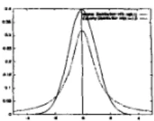
Figure 2: Comparisons of Gaussian and Cauchy distributions.
mutation. This technique performs well in parameter opti- mization problems. It is accomplished by first mutating step size wj. Next the connection link s:j is mutated by adding a
normally distributed random value with zero and w j as expec-
tation and standard deviation, respectively. This operator is realized by using the following equations (3) and (4).
Wj” = Wj”
.
[T’.
N(O,1>+
T.
Nj(0, I)] (3)x; = zp+w; .Nj(O,l), (4)
where N(0,l) is a normal distribution with mean 0 and stan- dard deviation 1. The solid line in Fig. 2 shows the density distribution of N(0,l). In addition, Nj(0,l) is a normaliza- tion distribution for the jth connection link. In our experi- ments, T and
7’
are set to (&%)-‘ and @)-’, respec-tively.
Self-adaptive Cauchy mutation: Cauchy density distri- bution is the dash line in Fig. 2 and is defined as follows:
where t is a scale parameter [211. The behavior of self- adaptive Cauchy mutation is $exactly the same as self-adaptive Gaussian mutation except Cauchy distribution replaces the normal distribution. Restated, the step size is controlled by using the similar equation in (6) and then the connection link xj is mutated by adding a Cauchy distributed random value with y5j as standard deviation. Self-adaptive Cauchy mutation is given by (6) and (7).
y5c 3 =
?+5;
ezp[T’.
N(0,l)+
T-
N j ( 0 , l)] (6)z; = 2; +?)j”.Cj(t), (7)
where C(t) is aCauchy probability distribution function with parameter t. In our experiments, t is 1.
Decreasing-based mutations: The decreasing-based Gaussian mutation and decreasing-based Cauchy mutation share the same step-size vector
5.
It is decreased by a de- creasing rate 7 , O+
y+
l. These two mutations use two fol- lowing (9) and (10) to mutate connection links, respectively.U; = 7.g; (8)
z; = 2;
+
U; * Nj(0,l) (9)z; = z;+Uj”.cj(l), (10)
where 7 is 0.95 in our experiments. According to (3), (6), and (8), two interesting phenomena are observed. First, (8) can
save computational time because it is multiplication; in addi- tion, (3) and (6) must compute a normal distribution function as well
as
an exponential function. Second, the search behav- ior of decreasing-based mutation markedly differs from self- adaptive mutations because (8) decreases the step sizes by a fixed rate; however (3) and (6) adapt step sizes by a stochastic approach.2.5 Selections
FCEA uses four selections: recombination selection, fam- ily selection, replacement selection, and population selection. FCEA employs recombination selection to select two individ- uals for recombination. One is “family father” and the other is randomly selected from the population. Family selection selects the one with best objective value from the L offspring that are generated from the same “family father”. The best children population set is then formed by repeatedly applying the procedure. In
our
three mutation stages except for the decreasing-based Gaussian mutation stage, FCEA employs replacement selection to select the one with better objective value from “family father” and its best child that is selected by family selection. Combining family selection and replace- ment selection is usually viewed as a local search procedure. Population selection selects the best N individuals from the union set formed by the parent population set and best chil- dren population set. Population selection resembles ( p+
p)-ES used by traditional evolution strategies. 2.6 Adaptive
Rules
Controlling the step size heavily influences the perfomance of Gaussian and Cauchy mutations. FCEA constructs the re- lationship between self-adaptive mutations and decreasing- based mutations by combining deterministic, self-adaptive, and adaptive techniques to effectively control the step sizes of Gaussian and Cauchy mutations according to the adaptation classification [5]. Herein, these rules are summarized into A-rules, including A-adaptive-rule and A-decrease-rule, for self-adaptive mutations and D-rules, including D-decrease- rule and D-increase-rule, for decreasing-based mutations.
1. A-&@:
0 A-adaptive-rule: This_self-adaptive rule controls
the step sizes of v’and y5 according to (3) and (6). It is called a self-adaptive rule because the step- size vectors v’ and $ are directly encoded into a chromosome of an individual and undergo mu- tations and recombination. The rule is applied when the mutation is a self-adaptive one.
0 A-decrease-rule: ,The rule decreases the step-
size vectors v’ and $ of a “family parent” when the “family parent” is better than its best child gener- ated
t
y
applied family competition. Step sizes v’ and $ are adapted while self-adaptive Gaussian and self-adaptive Cauchy mutation are applied,respectively. The step sizes v’ and
4
are adapted in the following manner:w; = 7 ~ ; if ‘‘family parent” 3 is (1 1)
where 7 is the decreasing rate and 7 is 0.95 in our experiments.
better than its best child,
2. D-rules:
0 D-decrease-rule: The rule is a deterministic rule
because it decreases the step size ?t according to
(8). The rule is applied when the mutation is
a
decreasing-based one.0 D-increase-rule: This adaptive rule enlarges the
step size t3of the best child when family compe- tition is applied and the best child is better than its “family father” in two self-adaptive mutation stages. It updates the step sizes as follows: oj”
=Pvh,,,,
i f U; 4Pv~,,,,
and the best child c‘is better than its ”family parent” Z,
(12) where v’ is the step-size vector of the best child;
vLe,,,
is the mean value of the vector v’; and p is 0.2 in our experiments.FCEA successfully combines self-adaptive mutations and decreasing-based mutations via A-rules and D-rules to en- hance the performance. Later we demonstrate how these rules can enhance the performance of FCEA.
3 Boolean Functions Learning
FCEA is applied to optimize the connection weights for two well-lmown Boolean function problems [E]
.
To compare with previous works, FCEA uses standard fully connected networks structures which have a hidden layer with a bias neuron. These two problems are describedas
follows:1. Xor: An ANN has 2 input nodes, 2 hidden nodes, and 1 output node. There are 9 connection weights and 4
input patterns. The output value is the Exclusive OR of the input bits.
2. Addition: An ANN has 4 input nodes, 4 hidden nodes, and 3 output nodes. These are 35 connection weights and 16 input patterns. The output pattern is the result of the sum of the two 2-bits input strings.
Herein, binary input patterns are used and a network is trained to generate output values ranging from 0 to 1. The fitness function of a network is based on mean square error and is given below
Table 1: Comparison the results of FCEA with previous works on two Boolean functions.
I
Method1
xorI
Addition1
Evolutionary 2000.0 Promammine f41 (100%) N/A Algorithm [18] Adaptive Genetic1
StandardGenetic1
6120I
I
(80%) N/A 3473 GENITOR 1191 GENITOR II [191tGENITOR is a well-known modified genetic algorithm. tGENITOR II is a distributed version of GENITOR. t(N/A denotes not available in the literature.) $The values in () is the successful classified rate.
(93%)
where Ohj and O& denote, respetively, the output value and training value of the j t h output neuron for the kth input pat- tern; m is the number of input pattern; and No is the number of output neuron. A training input pattern is classified cor- rectly if the tolerance of
[&
-
O&I is below 0.1 for each output neuron. A network is convergent if the network clas- sifies all the training input patterns.Evolution begins by initializing all the connection weights z' of each network to random values between -0.1 and 0.1. The initial values of step sizes for decreasing-based mu- tations, self-adaptive Gaussian mutation, and self-adaptive Cauchy mutation are 1.0, 0.25, and 0.25, respectively. The family competition length Ld and La in the decreasing-based stages and self-adaptive stages are 3 and 9, respectively. In this case, FCEA generates 720 networks, i.e. (3+9+9+3).30, in one generation if the population size is 30. The population size is 10 for Xor and is 30 for addition problems. The rate of recombination is 0.2. These parameter values except for the population size are applied eo dl problems addressed herein. Table 1 compares our FCEA, evolutionary programming [4],
and
genetic algorithm[HI,
[19]on
the Boolean func- tions. Detailed implementation of these compared ap- proaches can be found in the original papers. According to pertinent literature, the performance of their evolutionary al- gorithms is competitive with back propagation. FCEA is ex- ecuted 50 runs for each problem and is up to 500000 function evaluations, i.e., the number of generated offspring, for each run. FCEA can solve J 1 Boolean functions within reasonable function evaluations; the successful classified rates are 96% for Addition problem.Standard evolutionary algorithms, such as simple genetic algorithm [18] and (1+6)-ES [16], cannot completely solve Xor problem for all puns. The modified evolutionary algo- rithms [ 161, [ 181 can resolve simple problems, such
as
Xor.Figure 3: Artificial ant problems: "John Muir Trail".
However, they only solve several simple problems. GENI- TOR needed only around 500 recombination to resolve Xor problem. However, it required a population of 5000 and 2 million function evaluations to solve 2-bit adder and the clas- sified rate is only 56%. These results indicates that although efficient for simple problems, these evolutionary algorithms can not solve complicated problems, such as Addition prob- lems. GENITOR
II,
a distributed version ofGENITOR,
can increase classified rate to 93% in the Addition problem. How- ever, its population size is also 5000 and the number of func- tion evaluations also reaches 2 million. In contrast to these approaches, FCEA only needs 256464 function evaluations and the successfully classified rate is up to 96% by using small population size, i.e., 30, for Addition problem. These results demonstrate that FCEA is a robust approach to train forward networks for Boolean functions learning.4
The Ant
Problem
This study applies FCEA to experiment on complex search and collection task that is the tracker task "John Muir Trail" [8]. In this problems. a simulated ant is placed on a two- dimensional toroidal grid that contains a trail of food. The ant traverses the grid to collect any food encountered along the trail. This task attempts to train a neural network, i.e., a simulated ant, that collects the maximum number of pieces of food during the given time steps.
Fig.3
shows this trail. Each black box in the trail stands for a food unit. According to the environment of [8], the ant stands on one cell, facing one of the cardinal dwtions; it can sense only the cell ahead of it. After sensing the cell ahead of it, the ant must take one of four actions: move forward one step, turn right 90°, turn left go", and no-op (do nothing). In the optimal trail of the "John Muir Trail", there are 89 food cells, 38 no food cells, and 20 turns. So, the number of minimum steps for eating all food is 147 time steps. On the other hand. an ant requires at least 165 time steps to completely travel the optimal trail of the "Santa Fe Trial".f
Figure 4: The typical convergent curve of “John Muir Trail” problems.
Figure 5: The typical search behavior of a simulated ant con- trolled by our evolved neural controller for “John Muir Trail” ant problem.
of [SI. That investigation not only used finite state machines and recurrent neural networks to represent the problem, but also used the traditional bit-string genetic algorithm to train the structures. Each simulated ant is controlled by a network having two input nodes and four output nodes. The “food” in- put is 1 when food is present in the cell ahead of the ant; and the second ”no-food” is 1 in the absence of food in the cell in front of the ant. Each output unit corresponds to a unique action: move forward one step, turn right 90°, turn left 90°,
or no-op. Each input node is connected to each of the five hidden nodes and to each of the four output nodes. The five hidden nodes are fully connected in the hidden layer. There- fore, this structure is a full connection with shortcut recurrent neural network; its total number of links with bias input is 72. To compare with previous results, the fitness is defined
the number of pieces of food eaten within 200 time steps for “John
Muir
Trail”.Fig.4 displays the convergence curve of the ant problems. Fig.4 indicates that FCEA only requires about 12,000 func- tion evaluations to train a neural controller to find 82 food pieces within 200 time steps. To find 85 and 88 food pieces within 200 time steps, FCEA then requires about 35000 and 58000 function evaluations. FCEA on average found 81,87, and 88 food pieces within 200 time steps about 2oooO,65000, and 8oooO function evaluations, respectively. “John Muir Trail” was tested over 25 runs and the rate of success of find- ing 89 food pieces was 80%. The remaining 20% of runs the ant foraged at least 86 food pieces. The successful rate can be improved to 96% when the population is 100 and the number of function evaluations is 500,000.
Table 2: Comparison among genetic algorithm, evolutionary programming, and our FCEA on ”John Muir Trail” ant prob- lem.
k I
Fig.5 depicts a typical search behavior and the traveled path of a simulated ant that is controlled by our evolved neural network. The number of the cell is the time step to eat the food. The symbol
’*’
denotes a cell traveled byan
ant when the cell is empty. Fig.5 indicate that the ant requires 195 time steps to seek all 89 food pieces in the environment of “John Muir Trail”.Table 2 compares our FCEA, evolutionary programming [ 141, and genetic algorithm 181 on the “John Muir Trail” ant problem. Jefferson et al. used traditional genetic algorithms to solve “John Muir Trail”. That investigation encoded the problem with 448 bits and used a population of 65536 to achieve the task in 100 generations. Their approach required 6,553,600 networks to forage 89 food pieces exactly within 200 time steps. In contrast to Jefferson’s solution, our FCEA uses population sizes 50 and 100, and only requires about 126,000 and 284,000 function evaluations, respectively, to eat 89 food pieces within 195 time steps. Table 2 also indicates that FCEA perfoms better than evolutionary programming.
5
The Characteristics
of
FCEA
In this section, we briefly &scussed several characteristics of FCEA via experimental designs. Table 3 compares the ten approaches in term of 2-bits Adder functions and an ant problem. Each approach is a combination of operators applied in our FCEA: decreasing-based Gaussian mutation (MDG), self-adaptive Cauchy mutation ( M c ) , self-adaptive Gaussian mutation (MG), and decreasing-based Cauchy mu- tation (MDc). For example, the M c approach only uses self- adaptive Cauchy mutation; the MDG
+
MC approach inte- grates decreasing-based Gaussian mutation with self-adaptive Cauchy mutation and it also applied the control rules. The FCL~FCEA approach is unique case of our FCEA because the family competition lengths (Ld and L a ) is set to 1. The NCRFCEA approach is also a unique case of our FCEA but it does not apply adaptive rules, i.e., A-decrease-rule and D- increase-rule. The final approach in Table 3 is a standard evo- lution strategy i.e., ( p+
X)-ES, where p is 20 and X is 120. Each approach executes 50 runs for Boolean Functions; and 25 runs for the ant problem. The maximum numbers of func- tion evaluations of each run on Boolean functions and the ailtMethods
problem are 500,000 and 250,000, respectively. The value in the parenthesis in the ant problem denotes the average num- ber of food pieces eaten.
We observe several properties according to these experi- mental results of Table 3 and Fig. 6.
e Each mutation operator in FCEA has different perfor- mance on the seCected problems. These results indicate that each operator has different search behavior.
0 Generally, the approaches of a combination of multiple
mutations perform better than the approaches of unary- operator mutation and they do not increase proportion- ally on the number of function evaluations. For ex- ample, our FCEA that combines MDG, Mc, MG, and MDC has the best performance among all approaches on all testing problems. Nevertheless, the number of function evaluations of FCEA is not larger than other approaches for all testing problems.
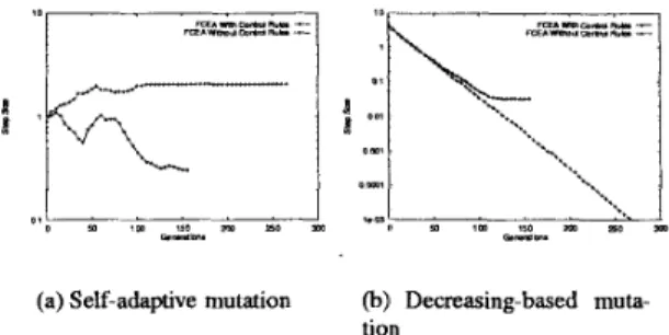
e The control rules of step sizes are useful because
NCRFCEA
perfoms worst than FCEA. Fig. 6(b) in- dicates that the step size ( 0 ) of decreasing-based mu-tation becomes small while FCEA does not apply D- increase-rule. Fig. q a ) indicates that the step size of self-adaptive Gaussian mutation is too large to improve solution while FCEA does not apply A-decrease-rule.
Q The family Competition length is a one of critical fac-
tors of FCEA
m
obtain better performance for com- Addition Jefferson'sAnt Problem
(a) Self-adaptive mutation (b) Demasing-based muta- tion
Figure 6: The comparison of average step size between FCEA with adaptive rules and FCEA without adaptive rules on ant problem
plex problems. For example, FCEA have to enlarge the length in order to solve ant problems.
e Cauchy mutations perform better than Gaussian muta- tions on training neural networks.
6 Conclusions
This study has demonstrated that FCEA is an efficient ap- proach for training neural networks. The proposed algorithm combines decreasing-based mutations with self-adaptive mu- tations to enhance the performance based on family compe- tition and adaptive rules. Our FCEA is able to balance the exploitation and exploration of search ability. Results from Boolean functions and an ant problems confirm the flexibility and robusmess of such an evolutionary approach.
A global optimization method must consist of both global and local search strategies. For our FCEA, the decreasing- based mutation with large initial step size are global search strategies and self-adaptive mutations with family compe- tition procedure and replacement selection are local search strategies. Cauchy mutations are attention to be used in global search strategies than Gaussian mutations as demonstrated in the proposed approach. These mutation operators can be inte- grated to closely cooperate with each other. These smoothly integrated strategies make our FCEA applicable to train neu- ral networks for various applications as well as to solve vari- ous numeric optimization problems. Under appropriate con- ditions, FCEA is able to converge to a global solution.
In summary, experiments in these well-known problems verify that the proposed approach consistently performs more robustly than other algorithms, such as genetic algorithms, evolution strategies, and evolutionary programming. We be- lieve that the flexibility and robustness of our FCEA makes it a highly effective global optimization tool.
Bibliography
113 T. Blck, F. Hoffmeister, and H-P. Schwefel. A survey of evolution strategies. In Proc. Fourth Int. Con5 on Genetic Algorithms, pages 2-9,199 1.
[23 Y. Davidor. Epistasis variance: Suitability of a represen- tation to genetic algorithms. Complex Systems, 4:368-
383,1990.
[3] L. J. Eshelman and J. D. Schaffer. Real-coded genetic algorithms and interval-schemata. In L. D. Whitley, edi- tor, Foundations of Genetic Algorithm, volume 2, pages
187-202. Morgan Kaufmann Publishers, Inc., 1993. [4] D. B. Fogel, L. J. Fogel, and V. W. Porto. Evolving
neural networks. Biological Cybernetics, 63:487-193,
1990.
[5] R. Hinterding, 2. Michalewicz, and A. E. Eiben. Adap- tation in evolutionary computation: A survey. In Proc.
of IEEE Con5 on Evolutionary Computation, pages 65-
69, 1997.
[6] John H. Holland, Adaptation in natural and artificial Jystems. The University of Michigan Press, Ann Arbor,
MI, 1975.
171 K. Hornik. Approximation capabilities of multilayer feedforward networks. Neural Networks, 4:25 1-257,
1991.
[8] D. Jefferson, R. Collins, C. Cooperand M. Dyer, M. Flowers, R. Korf, C. Taylor, and A. Wang. Evo- lution as a theme in artificial life: The genesysltracker system. In Artijicial L$e 11: Proc. of the Workshop on Artificial Life. pages 549-577,1990.
[9] R. P. Lippmann. An introduction to computing with neural nets. IEEE ASSP Magazine, pages 4-22,1987.
[lo] J. R. McDonnell
and
D.
Waagen. Evolving recurrent perceptrons for time-series modeling, IEEE Trans. on Neural Networks, 5( 1):24-38, 1994.1113 D. J. Montana and L. Davis. Training feedforward neural networks using genetic algorithms. In Proc. of Eleventh Int. Joint Con$ on Artificial Intelligence, pages
[121 D. E. Rumelhart, G. E. Hinton, and R. J. Williams. Learning internal representations by error propagation. In D.E. Rumelhart and J. L. McClelland, editors, Pur- allel Distributed Processing: Explorations in the Mi- crostructures of Cognition, pages 3 18-362. Cambridge,
MA: MIT Press, 1986.
Cl31 R. Salomon. Scaling behavior of the evolution strat- egy when evolving neuronal control architectures for autonomous agents. In P. J. Angeline et al., editor, the
762-767,1989.
Lecture Notes in Computer Science: Evolutionary Pro- gramming VI, pages 47-57,1997.
1141 P. J. Angeline G. M. Saunders and J. B. Pollack. An evolutionary algorithm that constructs recurrent neural networks. IEEE Trans. on Neural Networks, 5( 1):54-
65, 1994.
1151 J. D. Schaffer, D. Whitley, and L. J. Eshelman. Com- binations of genetic algorithms and neural networks: A survey of the state of the art. In Proc. oflnt. workshop on Combinations of Genetic Algorithms and Neural Net- works, pages 1-37,1992.
[16] M. Scholz. A learning strategy for neural networks based on a modified evolutionary strategy. In Paral- lel Problem Solving from Nature-Proc. 1st Workshop PPSN I (Lecture Notes in Computer Science), volume
496, pages 316318,1991.
puter Models. Chichester: Wiley, 1981.
[ 171 Hans-Paul Schwefel. Numerical Optimization of Com-
[ 181 M. Srinivas and L. M. Patnaik. Adaptive probabilities of crossover and mutation in genetic algorithms. IEEE Trans. Systems, Man, and Cybernetics, 24(4):656-667,
1994.
[19] D. Whitley, T. Starkweather, and C. Bogart. Genetic algorithms and neural networks: Optimizing connec- tions and connectivity. Parallel Computing, 14:347-
361,1990.
[20] J. M. Yang, C. Y. Kao, and J. T. Horng. A continu- ous genetic algorithm for global optimization, In Proc.
of the Seventh Int. Con$ on Genetic Algorithms, pages
230-237,1997.
E211 X. Yao and Y. Liu. Fast evolutionary programming. In
Pmc. of the Fifth Annual Con5 on Evolutionary Pm- gramrning, pages 451460,1996.