Phase Separation and Persistent
Magnetoresistive Memory Effect in
La
0.375
Pr
0.25
Ca
0.375
MnO
3
Thin Films
研 究 生 : 蔡於璁
指導教授 : 莊振益教授
Table of Contents
(1) Abstract 1
(2) Chap. 1 Introduction 2
(3) Chap. 2 Fundamental Phonomenologies of Colossal Magnetic-Resistance (CMR ) 5 Materials
a. Phenomenology of CMR Materials 5
b. The Double-Exchange Model 6
c. Perovskite Structures & the Jahn-Teller effect 7
d. Phase Separation (PS) 10
e. Percolation 11
(4) Chap. 3 Experiments 12
a. Sample Preparation 12
(a) Target Fabrication 12
(b) Pulse Laser Deposition (PLD) 13
b. Characterization of Thin Film 15
(a) X-ray Diffraction (XRD) 15
(b) Temperature-dependent Transport 16
(c) Magnetization-Temperature Dependence 19
(d) X-ray Absorption Near Edge Spectroscopy (XANES) 21 c. Time Relaxation Behavior of Persistent Magneto-resistive Memory Effect 26
(5) Chap. 4 Results and Discussions 29
a. Persistent Magnetoresistive Memory Effect (PMME) on LPCMO thin film 29 (a) Anisotropy of Persistent Mangetoresistive Memory Effect (PMME) 29 (b) The Quenched Hth and The “Melting” Magnetic Filed Hm 34
b. Time-relaxation at Various Temperature Regimes 40 c. Metastable Resistance-temperature (RT) Dependence 51 d. R-H Oscillation Experiments at Various Temperatures 54
(6) Chap. 5 Summary and Conclusions 58
Abstract
Phase separation (PS) theory has drawn intensive attention in explaining the colossal magnetoresistance (CMR) effects nowadays. However, although displaying the same CMR phenomena as La1-xCaxMnO3(LCMO), (La1-x-yPrx)CayMnO3 (LPCMO) shows
another tremendous characteristics: a hysteresis in cooling and subsequent warming in both temperature-dependent resistance (R(T)) and magnetization (M(T))! In this thesis, aware of the more glassy-separated phase existences in LPCMO, we presume this hysteresis resulting from the long time relaxation behavior. As a consequence, we conducted a detailed study on the persistent magnetoresistive memory effect (PMME), which is believed to be intimately related to the detailed process toward to equilibrium state of a glassy phase coexistent system. The quality of the LCMO and LPCMO samples was carefully characterized by measuring the R(T) and M(T). The crystalline structure and electronic structure of the films were checked by x-ray diffraction (XRD) and x-ray absorption near edge (XANE) spectroscopy. In particular, LPCMO thin film, showing CMR effect, was taken to conduct temperature-dependent PPME experiments.
From the results, we obtained the equilibrium states of resistance of LPCMO at various temperatures, proposed a picture within a phase-size-related PS regime, and explained this glassy phase coexist system different with the not-glassy phase coexist system in LCMO.
Chap.1 Introduction
Though the first report of manganites was published in 1950 [1], it was not until about a decade ago that manganites started to draw tremendous attention from both the
academic and industrial areas. The main reason that revives these extensive research interests on manganites is largely due to the “colossal” magnetoresistance (CMR)—a MR ratio over 106 % obtained in mid-1990s. [2]. Zener first proposed his seminal double-exchange (DE) model to describe the simultaneous abrupt changes in the
temperature-dependent behaviors in electric transport and magnetic properties that were later coined as CMR [3]. However, as pointed out by Millis et al. [4], the DE model alone was not enough to give a quantities account on the experimentally observed CMR effect. By considering the crystal structure and the influence of Coulombic interaction of CMR materials, the Jahn Teller effect was introduced and probed [4-7]. More recently besides the DE model and the incorporation of Jahn-Teller effect developed in early days, nowadays the phase separation (PS) scenarios have been put forth as alternatives in explaining CMR effects. [8-15]
In this study, we tried to unveil the influence of PS nature on the electric transport of La0.375Pr0.25Ca0.375MnO3 (LPCMO) thin film, one of well-characterized CMR materials
[16-22]. In this material the time-relaxation behavior of resistance at various applied fields may reflect a significant phenomenon associated with the competition between
charge ordering (CO) and ferromagnetic-metal (FM) phases especially near the transitions. It denotes that the resistance continuously changes upon time after the disturbing factors ceased to acting may have been the process approaching the
equilibrium distribution of coexisting phases. [23-26] This behavior observed in LPCMO is apparently a strong support to the PS model, especially when we are looking for the equilibrium state at various temperatures. The importance of the equilibrium state cannot be over emphasized since the equilibrium state is the ground base of theoretical models aimed to interpreting the exotic yet frequently variable transport behaviors exhibited in the family of CMR manganites. Nevertheless, measurement of the actual equilibrium resistance of LPCMO is a difficult, if not impossible, job in lab, since the relaxation time is usually way too long for realistic to laboratory experiments. As a consequence, albeit over fifty years since CMR materials were discovered, only few indirect experiment data showed the probable equilibrium state of temperature-dependent resistance (R(T)) in LPCMO by measuring the persistent magnetoresistive memory effect, in a narrow temperature region. Undoubtedly, the discussion or study limited in that region is not adequate to lend a complete interpretation of transport characteristics of LPCMO. In this study we conducted systematic measurement of persist magnetoresistive memory effect (PMME) at various temperatures and applied fields. We then establish equilibrium state of the resistance of LPCMO over a wide range of temperatures and compared that with
the phase separation evolution process as depicted in Fig. 1[14]. We focus on the y=0.25 Pr doping concentration which has been demonstrated to have phases evolution from two short range (s-r) phases to final two long range phases with decreasing temperatures. Furthermore, the evolution of phases was evidently supported from the observation of the resistance response to applied magnetic filed oscillation.
Fig.1 <rA> donates the average ionic size. “y” is doping concentration of Pr. The lower
plot reveals different phase-coexistence at various temperatures. The red line is the guide of the eye for y=0.25. [14]
Chap. 2 Fundamental Phenomenologies of CMR materials
a. Phenomenology of CMR Materials
Magneto-resistance (MR) refers to the resistance changes of material in response to the applied magnetic fields. The MR ratio is defined as follows:
MR 0 0 R R R ratio= H − , (1)
where RH is the resistance measured under an applied magnetic field and R0 is the
resistance obtained at zero field. The MR phenomenon has been the subject for a great deal of recent research interest, because of the improvement and invention of
commercially available technologies – magnetic sensors, magnetic recording heads and magnetic memories, to name a few. There have been many kinds of MRs (AMR, TMR, GMR) studied and applied for years, each with distinctly different transport mechanisms. The colossal magneto-resistance (CMR) we discuss in this study is named because the MR exhibited is “colossal” as compared to other MR effects. For example, the MR ratio of “giant” magneto-resistance (GMR) is approximately 10~30%, while the MR ratio of certain manganites can be about 1500%! As an example, in Fig. 2, we show the typical CMR behaviors as a function of the applied field for our LPCMO films.
0 50 100 150 200 250 300 350 0 2000 4000 6000 8000 10000 12000 14000 R(oh m) T(K) 0T 1T 3T 5T 8T LPCMO
Fig.2 The resistance-temperature dependence at various magnetic applied field of LPCMO thin film is displayed. The plot shows a huge MR ratio (98%) at 175k.
b. The Double-Exchange Model
To explain the simultaneous occurrence of arising ferromagnetism and insulating to metallic transport behaviors in manganites, an indirect coupling, between the electrons residing at the incomplete d-shells of Mn is realized, via conduction electrons by hopping around Mn-O-Mn configurations. Since the coupling is indirect, the electron hopping must occur twice from Mn through O, to another Mn, it was termed as a
“double-exchange” mechanism as illustrated schematically in Fig.3. Zener stated that for each Mn ion, the incomplete d-shells must be occupied by electrons in accordance to the Hund’s rule, which means that unpaired spins in d-shells of each Mn ion are all aligned to maximize the magnetic moment [3]. It is conceived that if the net spins of the
incomplete d-shells are all aligned parallel, i.e. in the ferromagnetic state, conduction electrons would be able to lower their kinetic energy and conduct electricity more easily due to the minimization of spin scattering.
Fig.2 The conduction electron’s “double exchange” is displayed here twice, suggesting the process of electric transport along with the magnetic spin alignment.
c. Perovskite Structures & the Jahn Teller effect
However, the DE model failed to interpret the CMR phenomena in a quantitative manner [27]. The polaron mechanism along with phonons or magnons was proposed in trying to account for the discrepancies left by the DE model [5-7,28]. The crystal structure of manganites is belong to a lattice system generally called as perovskite structure [29](Fig.4). Apparently, since the electron hopping process only involves Mn and O ions, if we exclude other ions, an MnO6 octahedral cage emerges. Now let’s recall
the electronic configuration of d-shells shown in Fig.5. Corresponding to six O ions around Mn ion, we can see that the degeneracy of Mn d-level will be lifted and broken
2
x
d −
into two groups, one identified as eg band consisting of and the other
identified as t
2 2 2, 3z r
y d −
2g band consisting of dxy, dyz, dxz orbitals. It will be clearer if we take a look
at the shapes of these orbitals. The overlapped area of with O ion is larger
than that between d
2 2 2 2 y , 3z r x d d − −
xy, dyz, dxz. and O ion. The Columb repulsion naturally explains the
broken degeneracy and that the eg band is at the higher energy level. This is also referred
to as the crystal field effect [30]. Moreover, the degeneracy of the two orbitals in the eg
band can be further lifted because of the Jahn-Teller distortion (JTD)[4,7], namely the stretch along z-axis of MnO6, as depicted in Fig.6. The occurrence of JTD is driven by
the additional lowering of the ground state energy. With the JTD, the state will
overlap less area with O ion, leading to a lower-energy ground state. Similarly, the
will be forced to a higher energy level as a result of the increasing overlapped-area.
It is worth noting that JTD only happened in the situation of MnO
2 2 3z r d − 2 2 y x d − 6 octehedra with
as JTD only affects the electron on e
+ 3 .
Mn g state where there are four electrons in
d-shells. MnO6 octehedra with will not distort, attributed to the five electrons fully occupying spin-up states. As to MnO
+ 2 Mn
6 octehedra with , the JTD won’t lower the
energy because there is no electron in the e
+ 4 Mn
Fig.4 The diagram of perovskite structure displays the position of each ions.
Fig.5 The electronic configuration of d-shells of Mn includes 3dx2−y2and 3dx2−y2
belonging to eg band, and 3dxy, 3dxz and 3dyz belonging to t2g band. The crystal field
Fig.6 Jahn-Teller distortion stretches the z-axis of MnO6, lowering the energy of
ground state.
d. Phase Separation (PS)
Phase separation (PS), a manifestation of electronic inhomogeneities in manganites, has drawn increasing attention from researchers recently [31-33]. In this scenario, two distinct phases with different magnetical and electronic structures coexist and compete with each other. It is this competing behavior that dominates the electronic and magnetic transport. Theoretical calculations considering PS have been carried out, for example, for one-orbital model [32]. Moreover, many experiment results suggested that the
inhomogeneities in manganites system in various length scales, such as nanometer clusters and micrometer ones. As an example, Fig. 7 shows the scanning tunneling microscopy (STM) works displaying regions with different conductivities for La0.7Ca0.3MnO3 films in ferromagnetic-metallic state [34].
Fig.7 The phase separation of La0.7Ca0.3MnO3 thin film at T=88 K is observed from
STM work. [34]
e. Percolation
To account for the electric transport behavior within the context of PS model the percolation mechanism was developed with PS model. The main idea of percolation is ”sufficient links.” First of all, we regard the amounts of insulating and conducting “phases” as two different links in a two-dimension square, shown schematically in Fig.8. The amount of conducting phase grows as the temperature decreases. As a consequence, the conducting paths, reach to a critical portion of the square, forming a metallic
conducting path for electrons to transport. This is how percolation theory demonstrates the sudden drop of resistivity at the emergence of sudden increase of magnetization due to the ferromagnetic transition at the Curie temperature Tc [32].
Fig.8 f: the fraction of metal phase. Dark and thicker lines represent the metal links. (a)f=0.4,insulating(b)f=0.7,conducting.[35]
Chap. 3 Experiments
a. Sample Preparation
(a)Target FabricationWe synthesized the La0.375Pr0.25Ca0.375MnO3 (12g) and La0.625Ca0.375MnO3 (12g)targets
for the need of the pulse laser deposition. The method we applied is a standard solid-state route. Take La0.375Pr0.25Ca0.375MnO3 target for example, starting from preheated MnCO3,
Pr6O11, CaCO3, and La2O3 powders, we mixed them together with proportions of aimed
stoichiometry -MnCO3(6.720g), Pr6O11(2.487g), CaCO3(2.194g), and La2O3(3.571g)-
and heated this mixture to promote reactions among the constituents at 1200℃ for 8 hours; the solidified mixture was then grinded and pressed using a mold to form the target body; the target body was heated again at 1250℃ for 12 hours. This final procedure was repeated three times with an incremental heating temperature of 50℃ each time. The final sintering process was conducted at 1400℃ and furnace cooled over
several hours to room temperature. La0.625Ca0.375MnO3 target was fabricateded by the
same method, as well.
(b) Pulse Laser Deposition (PLD)
Briefly, the basic concept of pulse laser deposition (PLD) is to apply pulsed intense photons accompanied with large energy to ablate the materials form the target and deposit it onto the chosen substrate. In practice, a successful PLD fabrication requires correct conditions, which includes the deposition temperature, the output power of the excimer laser beam, the pressure of O2, and the choice of substrates. As to our samples,
La0.375Pr0.25Ca0.375MnO3 and La0.625Ca0.375MnO3 thin films, the PLD fabrication
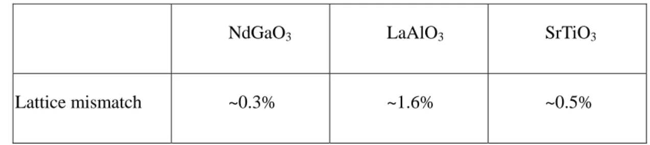
procedures are as following: first we chose NdGaO3 as our substrates for its lattice
constant (3.86 anstrom) being closest to our materials (3.87 anstrom) as compared to that of LaAlO3 and SrTiO3 (Table 1). The scheme of the PLD set-up is shown in Fig.9 with a
base pressure of 2×10⁻⁵ torr. We precisely tuned the O2 pressure to 0.3 torr by needle
valve and controlled the deposition temperature at 700℃ with the heater behind the holder and the thermal couple imbedded in the holder on which the NdGaO3 substrate
was attached. The 248 nm KrF excimer laser pulses with 350 mJ and repetition rate 3 Hz was then guided into the chamber by UV mirrors and lens, as depicted in Fig.9.
Afterward, the film was cooled in 400 torr O2 environment to room temperature with the
films was about 250 nm with the LCMO being deposited at a slightly higher deposition temperature 720℃.
NdGaO3 LaAlO3 SrTiO3
Lattice mismatch ~0.3% ~1.6% ~0.5%
Table 1. Comparison of several substrates by lattice mismatch with LCMO/LPCMO lattice constant 3.87 anstrom.
b. Characterization of Thin Film
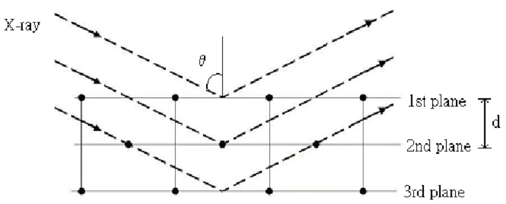
(a) X-ray Diffraction (XRD)X-ray diffraction (XRD) measurement has been a useful tool to check the crystal structure of samples. Based on Bragg diffraction condition:
nλ =2dsinθ (2) where n is an integer,λis the wavelength of the x-ray, d is the distance between
successive parallel planes, and θ is the angle between incident x-ray and the normal line of the lattice plane.
Fig. 10 The illustration of XRD process. θ denotes the angle between incident x-ray and the normal line of lattice planes.
In addition, the pattern of XRD also has to meet the requirement of the structure factors and atomic form factors. X-ray patterns of our samples are displayed in Fig.11, along with the pattern of the NdGaO3 substrate for comparison. Obviously we can assure
measurements of films grown with similar conditions it has been demonstrated that these PLD manganite films retained excellent epitaxial relations with the substrate..
5 10 15 20 25 30 35 40 45 50 55 60 65 LC MO(00 4 ) N GO(1 00) L C MO(002 ) LPC M O (002) N GO(2 00) Int e nsi ty (a. u. ) 2θ (degree) NGO LPCMO LCMO LP C M O(00 4)
Fig.11 XRD shows epitaxial relation between our films and NGO substrates. (b) Temperature-dependent transport
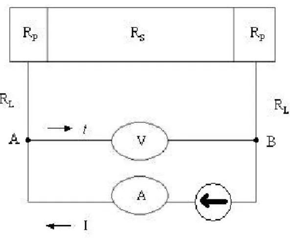
The standard four-probe configuration is employed to measure the resistance of samples. The traditional two-probe configuration (Fig.12) could leave us all the resistances (RM) from contact pads (RP), from lines (RL), and from the sample (RS):
(
)
P L S M P L S AB M R R R R I i I i I R R R i I I V R 2 2 0 2 2 ) ( + + = ⇒ ≈ − ⇒ ≈ + + × − = = Q (3)Fig. 12 The configuration of two-probe resistance measurement system. By separating current-source pads and voltage- meter pads, we can avoid the combined voltage-drop including pad resistance, line resistance and the sample resistance and measure the exact resistance of the sample. This method is generally referred as standard four-probe measurement (Fig.13). In this configuration:
(
)
(
)
S S M P L S AB M R I R I R I i I i I R R i R i I I V R = + × = ⇒ ≈ − ⇒ ≈ + × + × − = = 0 0 2 2 Q (4)The resistance-temperature dependences of LCMOand LPCMO thin films are displayed in Fig.14 and Fig.15. As shown in both samples, the resistance increases with decreasing temperature, indicative of an insulating behavior. Nevertheless, when the temperature reaches Tp, a sudden drop of resistance occurs at Tp, and the resistance kept
decreasing with the lowering temperature, revealing a typical metallic behavior.
Particularly, along with the process of cooling and subsequent warming, we observed the hysteresis phenomenon in LPCMOthin film.
0 50 100 150 200 250 300 0 50 100 150 200 250 300 350 400 cooling warming R(ohm) T(K) LCMO/NGO T p
0 50 100 150 200 250 300 350 0 2000 4000 6000 8000 10000 12000 14000 T(K) R( ohm) warming cooling LPCMO/NGO TP
Fig.15 The resistance-temperature dependence of LPCMO is plotted with Tp at 175K.
The plot shows the clear hysteresis of LPCMO. (c) Magnetization-Temperature Dependence
The temperature-dependent magnetization (M(T)) was measured using the Quantum Design Superconducting Quantum Interference Device (SQUID) system. Fig. 16 shows the M(T) result of LCMO, displaying a paramagnetic to ferromagnetic transition around T= 270K. On the other hand, Fig. 17 shows the M(T) of LPCMO film. It is evident that, similar to that observed in R(T), the M(T) of LPCMO also displays a clear hysteresis.
0. 0. 0. 0. 0. 0. 0. 0. 0. 0 50 100 150 200 250 300 0000 0002 0004 0006 0008 0010 0012 0014 0016 T(k) LCMO M(emu)
Fig.16 The magnetization-temperature (MT) dependence of LCMO is shown. The saturation of magnetization at low temperature indicates the FM.
0 50 100 150 200 250 300 0.0000 0.0001 0.0002 0.0003 0.0004 M( emu) T(k) warming cooling LPCMO
Fig.17 The temperature-dependent magnetization (MT) of LPCMO. Notice that in addition to the saturation of magnetization exhibited at low temperature, a significant hysteresis in M(T) is evident over a wide range of temperatures.
The dramatic variations in electrical and magneto properties accompanied with the paramagnetic-ferromagnetic transition at Tc and insulator-metal transition at Tp is
believed to be intimately associated with the electronic structure change of the perovskite manganites. In order to detect the electronic structures, the x-ray absorption spectroscopy (XAS) has become a rather important tool [39-45]. Fig. 18 illustrates the various
processes involved when an energetic photon is absorbed by the atoms. Essentially, the incident x-ray with the energy in the order of several hundred eV allowed the core level electrons of a particular atom of interest (A) to promote to the higher level (B) followed by dipole selection rule with no spin changes. As the excited electron relaxed back to the core level, the electron occupying at level B absorbed the energy from the relaxation and produced fluorescence photon, most of which further excited the Auger electron.
Therefore, we can obtain the spectrum from both fluorescence photon and Auger electrons and delineate the relevant electronic structure change due, for example, to environmental change of the particular ions.
Fig.18 The diagram shows the process of XAS. The incident x-ray excited the core electron and after the relaxation of the excited electron, the fluorescent photon and the Auger electron could be detected.
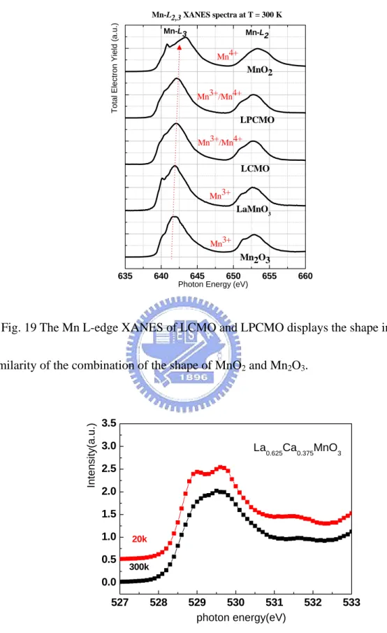
X-ray absorption near-edge spectroscopy (XANES) requires the high-energy spherical grating monochromater beamline, which is, in our case, at the National Synchrotron Radiation Research Center, Taiwan, to permit x-ray absorption for XANES. The base pressure in the spectrometer chamber was better than torr; the resolution of the spectra was 0.22eV controlled by the spherical grating monochromater; and the standard procedure to remove the background contribution and to normalize the intensity was adopted. Hereby, we first checked the Mn L-edge XANES of our samples as a fingerprint to assure the Mn ions consisting of both Mn
9
10−
3+
and Mn4+(Fig. 19). Comparing with the shape of the standard samples, Mn2O3 and MnO2, we can approximately regard
behavior occurring at low temperature at the pre-edge of O K-edge was intensely discussed by researchers, the O K-edge XANES of LCMO and LPCMO were displayed for comparison. As is evident from Fig. 20, the absorption peak of the O K-edge XANES shows the peak-splitting behavior at low temperature (LT) for the LCMO sample
(Fig.20). While for LPCMO sample such LT peak-splitting behavior is absent (Fig. 21). Among the models describing this splitting behavior, our results appear to support the picture chematically depicted in Fig. 22. In this picture, it is conceived that the JTD induces significant change in the electronic structure. At room temperature (RT), the larger JTD leads to the strong hybridization of the dx2−y2 state of eg(↑) band with the t2g
(↓) states; at low temperature (LT), the diminishing JTD leads to a much weaker hybridization and thus the dx2−y2 state of eg(↑) band is further separated from the t2g
(↓) states and is manifested as the peak splitting. It is possible that due to the smaller exchange interaction energy, the hybridization in LPCMO is so strong that the difference of JTD at RT and at LT could not be distinguished.
635 640 645 650 655 660 LaMnO3 LCMO LPCMO Mn3+ Mn3+/Mn4+ Mn3+/Mn4+ Mn3+ Mn4+ Total Ele c tron Yield ( a .u.)
Photon Energy (eV)
Mn-L3 Mn-L2
Mn2O3 MnO2
Mn-L2,3 XANES spectra at T = 300 K
Fig. 19 The Mn L-edge XANES of LCMO and LPCMO displays the shape in similarity of the combination of the shape of MnO2 and Mn2O3.
527 528 529 530 531 532 533 0.0 0.5 1.0 1.5 2.0 2.5 3.0 3.5 In tensi ty( a. u .) photon energy(eV) 20k 300k La0.625Ca0.375MnO3
Fig. 20 The temperature-dependent XANES of LCMO is displayed. We can observe the splitting behavior at 529.5 eV at T = 20 K, comparing to the peak at T = 300 K.
527 528 529 530 531 532 533 0.0 0.5 1.0 1.5 2.0 2.5 3.0 3.5 photon energy(eV) La0.375Pr0.25Ca0.375MnO3 Intens ity (a .u.) 300k 20k
Fig.21 The temperature-dependent XANES of LPCMO reveals the disappearance of the splitting behavior at T = 20 K.
Fig.22 The schematic diagram displays the process of breaking the degeneracy of Mn
3d states. In this model, the dx2−y2 state of eg(↑) states closely hybridized with the t2g (↓)
c. Time-relaxation Behavior Measurement
—The Persistent Magnetoresistive Memory Effect (PMME)
The resistance of LPCMO sample would relax with the elapsed time to the
equilibrium state below charge-ordering temperature. However, no matter the resistance increased or decreased upon time, the relaxation time period for laboratory experiments is too long. Due to the obstacle of waiting the sample to approach the equilibrium state, we adopted the method originally used by P. Levy et al. to perform experiments on this persistent magnetoresistive memory effect (PMME). [25]; This method is done as following. Under a cooling protocol to a certain temperature we applied a magnetic field to disturb the distribution of the coexisting phases; here it is to enhance the growth of the metallic phase. Then after removing the applied field, we measured the tendency of the resistance relaxation. Fig. 23 illustrates the procedures of this experiment. The resistance would not rejuvenate to its virgin value, if there exists the PMME. Furthermore,
depending on the magnitudes of applied field, two following situations could happen. Either the resistance decreased or increased as a function of time. A threshold field Hth is
then determined. By definition, after we applying field above Hth, the ulterior relaxation
of the resistance reversed its sign. Several models have been proposed to explain this phenomenon. One of the purposes of this study is to clarify the dominant mechanism leading to this phenomenon.
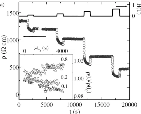
Fig. 23 The upper part of this diagram shows the appliance and removal of H with time evolution. The resistance changes upon this time period were measured. The inset indicates the reverse sign of the tendency.
In addition, this method could also help us find the equilibrium state of sample resistance at various temperatures because it must be lying somewhere between the minimum of the decreasing resistance and the maximum of the increasing one. Before we get into the detailed discussion of the PMME results, we first show the experimental results of LCMO and LPCMO respectively in Fig. 24 and Fig. 25. It is evident that complete rejuvenation of resistance in obtained for LCMO, indicating an absence of PMME for this material. On the contrary, for LPCMO, the also relaxation towards the equilibrium resistance is observed after the removal of the applied field. The behavior also is very much dependent on the strength of the applied field. Although it is not clear
at present the actual mechanism, giving rise to the difference between LCMO and LPCMO, it is, nevertheless, quite consistent with the hysteretic behavior of the R(T) and M(T) results described above. We suspect that, although both materials are found to have phase coexistent over wide range of temperatures, the formation of the coexistent phases may have very different natures. Namely, we note that in LCMO the coexisting phases are the parent paramagnetic insulating phase and newly formed ferromagnetic metallic phase. While for LPCMO, the phases transition involves a pair of new phases (the CO and FM phases) are formed from a single paramagnetic phases when temperature is lowered below TCO In any case, since the PMME is only observable in LPCMO, we will
focus on discussion of this effect on this particular material.
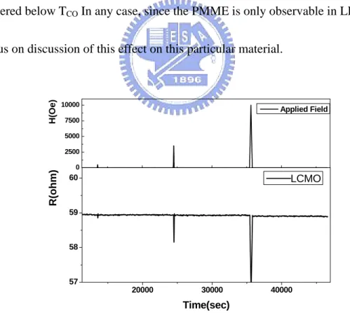
20000 30000 40000 57 58 59 60 0 2500 5000 7500 10000 R(ohm ) Time(sec) LCMO H( O e ) Applied Field
Fig. 24 The resistance remained almost the same after removals of different applied magnetic field impulses.
20000 30000 40000 10400 10800 0 2500 5000 7500 10000 R(o h m) Time(sec) LPCMO Applied Field H( O e )
Fig.25 The drop of the resistance did not rejuvenate to its original value after removal of the applied magnetic field impulses.
Chap. 4 Results and Discussions
a. Persistent Magnetoresistive Memory Effect (PMME) on LPCMO
thin film
(a)Anisotropy of Persistent Mangetoresistive Memory Effect (PMME)
In order to delineate the intrinsic characteristic of the epitaxial thin films, whether the anisotropy of applied magnetic field existed deserved to be confirmed. The experiment procedure is as following: we first cooled the sample to T= 174 K, the middle point of the R(T) hysteresis in zero applied field, at a constant rate of 3 K/ min; next, after waiting for 90 minutes for the resistance to relax, a small magnetic field of 200Oe was applied for another 90 minutes; then the magnetic field was removed and completed as
one 180-minute cycle. Same cycles were repeated with larger and larger magnetic field up to 1 Tesla. Fig. 26(a) shows the results for in-plane applied field. Notice that below a field denoted as Hth the relaxation is descending while above that an ascending relaxation
is evident. (See the circles shown in Fig. 26(a) and the enlarged version shown in Fig. 26(b).) For fields applied perpendicular to the film surface, similar behaviors were observed, except that Hth in this case is much larger (~1T) as compared to the in-plane
field (Hth~0.1T). 0 10000 20000 30000 40000 50000 0 2000 4000 6000 8000 10000 12000 0 2000 4000 6000 8000 10000 H(Oe) R( oh m) Time(sec) H in plane Hth
Fig.26 (a) The process of H-in-plane experiment with time evolution is illustrated. The drop of the resistance caused by magnetic field represents normal MR effect. We marked Hth as a threshold magnetic field that reversed the resistance relaxation tendency.
22000 23000 24000 25000 26000 7560 7580 7600 7620 7640 11000 12000 13000 14000 15000 9520 9540 9560 9580 9600 9620 R( ohm) Time(sec) R( ohm) Time(sec)
Fig.26 (b) The enlarged diagram illustrates the reversed tendency of resistance relaxation after removal of Hth.
0 10000 20000 30000 40000 0 2000 4000 6000 8000 10000 120000 5000 10000 R(ohm) Time(sec) H out of plane H(Oe) Hth
Fig.27 (a) The process of H-out-of-plane experiment with time evolution is illustrated. We discovered a larger Hth as shown.
43000 43500 44000 44500 45000 45500 46000 46500 47000 1340 1350 1360 1370 1380 1390 1400 32000 33000 34000 35000 36000 37000 7750 7755 7760 7765 7770 7775 R(ohm) R(ohm ) Time(sec) Time(sec)
Fig.27 (b) The enlarged diagram illustrates the reversed tendency of resistance relaxation after removal of Hth.
The anisotropy of the change and hence the subsequent relaxation of the resistance is believed to be related to the degree of magnetization in the sample. Therefore, we’ve measured the magnetization-H (M(H)) dependence at various temperatures. The results are summarized in Fig. 28. From diagrams displayed in Fig. 28, especially at low temperature (e.g. T= 10 K), we can discern the easy axis parallel to H in plane by clear hysteresis loop. It is reasonable now to infer that the different Hth exhibited in the two
applied directions is having the origin of the intrinsic anisotropy of our thin films. In the remaining of our discussion, we will focus on the results obtained for field applied in-plane.
-10000 -5000 0 5000 10000 -0.0006 -0.0004 -0.0002 0.0000 0.0002 0.0004 0.0006 M(e .m.u .) H(Oe) Magnetization10k Magnetization100k Magnetization174k Magnetization250k H in plane
Fig. 28(a) By applying H in plane, the hysteresis of MH dependence is shown. At lower temperature, the M saturation is larger along with a clearer hysteresis.
-10000 -5000 0 5000 10000 -0.0006 -0.0004 -0.0002 0.0000 0.0002 0.0004 0.0006 H out of plane Magnetization10k Magnetization100k Magnetization174k M( e.m.u.) H(Oe)
Fig. 28(b) By applying H out of plane, we can find no hysteresis behavior within same magnitude region of H. The lack of hysteresis indicates that when H is applied out of plane, it is hard-magnetization-direction for our sample.
(b)The Quenched Hth and The “Melting”Magnetic Filed Hm
It is notable that PMME only occurs at certain temperature with a cooling scheme. Upon cooling, the FM phase might not have enough time to reach its equilibrium distribution. Thus, when field H is applied, it may enhance the growth of FM phase and even drive it to exceed the equilibrium proportion. It is under such premise that we can conduct PMME experiment and observe the reverse tendency of resistance relaxation after after removing H. However, if we first cooled LPCMO thin film to low temperature, say T= 10K, the proportion of FM phase at low temperature, though still may not reach its equilibrium proportion, is much larger than that at higher temperatures. Upon warming, due to transformation lagging, FM phase continuously exceeded the
equilibrium proportion at certain temperature. In that case, we will not be able to observe the reverse tendency of resistance relaxation, and naturally we cannot define Hth—the
Hth is said to be quenched. The results at different temperatures at which R(T) displays
hysteresis namely from T=160 K to T=180 K are shown in Fig.29 (a) (T= 174 K), Fig. 30 (a) (T= 177K), and Fig. 31 (a)(T= 180K, inset shows the enlarged vision).
0 10000 20000 30000 40000 400 600 800 1000 1200 1400 1600 18000 5000 10000
H(Oe)
R(
ohm)
Time(sec)
T= 174 K
HmFig.29 (a) At T = 174 K, as the time evolved, the resistance tended to increase clearly. The noticeable sudden drop represented a strong MR effect, and the Hm is denoted.
28000 30000 32000 1510 1515 R(ohm) Time(sec)
H = 4000 Oe
38000 40000 42000 440 460 480 R(ohm) Time(sec)
H = 1 tesla
Fig.29 (c) When H > Hm, the relaxation tendency decreased.
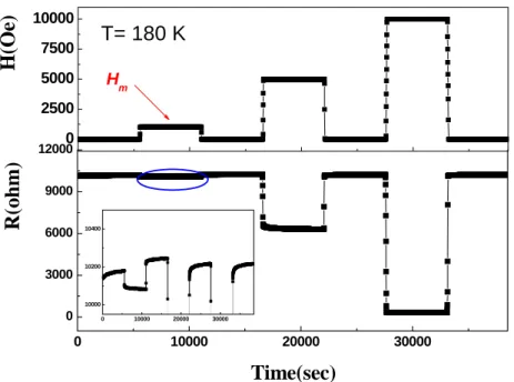
0 10000 20000 30000 40000 50000 0 2000 4000 6000 8000 10000 0 10000 20000 30000 H(Oe) R(ohm) Time(sec) T= 177 K Hm
Fig.30 (a) At T= 177 K, the sudden drop occurred with a smaller Hm. Below Hm the
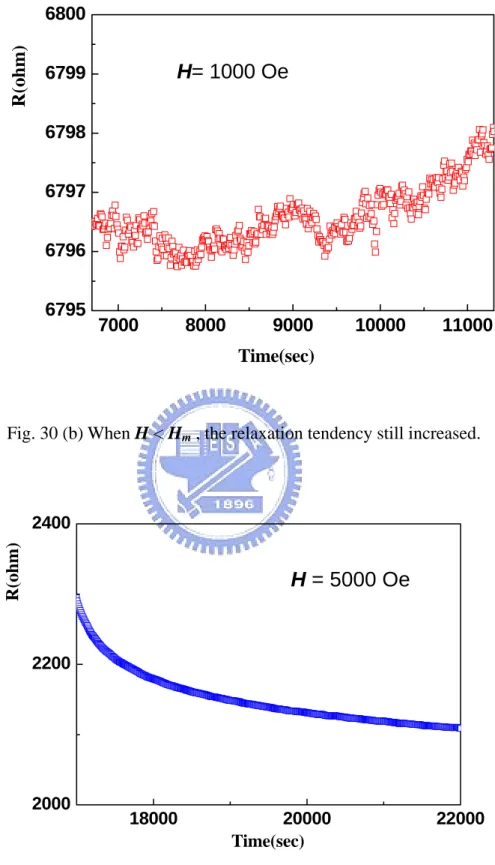
7000 8000 9000 10000 11000 6795 6796 6797 6798 6799 6800 R(o h m) Time(sec)
H= 1000 Oe
Fig. 30 (b) When H < Hm , the relaxation tendency still increased.
18000 20000 22000 2000 2200 2400 R(oh m) Time(sec)
H = 5000 Oe
0 10000 20000 30000 0 3000 6000 9000 120000 2500 5000 7500 10000 0 10000 20000 30000 10000 10200 10400 H( Oe ) R( o h m ) Time(sec) T= 180 K Hm
Fig. 31 (a) At T= 180 K, Hm was smaller but without a resistance drop. The inset shows
the enlarged vision of the resistance to scrutinize the relaxation tendency.
6000 8000 10000 10080 10090 10100 R(ohm) Time(sec) H = 1000 Oe
Interestingly, at different temperatures, we needed to apply certain magnetic field which is strong enough to “melt” the CO phase. As just mentioned above, the FM phase always exceeded its equilibrium proportion upon the warming scheme. On the other hand, the CO phase continuously grows to reach its equilibrium proportion upon
warming protocol. Therefore, we need a strong H, namely Hm, to suppress the growth of
CO phase or to “melt” the grown CO phases. This is how we define Hm: we observed the
relaxation tendency of resistance while the applied magnetic field was on. With larger and larger H, the tendency changed from ascending to descending. When the tendency just reversed its sign (shown in Fig. 29(c), Fig. 30(c), and Fig.31(b)), the threshold H was defined as Hm.
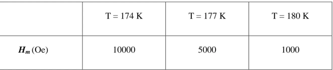
To compare the trend of Hm at various temperatures in this experiment, we tabulated
our data in Table 2. Recalling the resistance-temperature dependence shown in Fig. 15, we picked these three temperatures in the hysteresis region: at T= 174 K, the CO phases were still robust and far from its equilibrium proportion, so we needed larger magnetic force (Hm ~1T) to melt the CO phase; at T = 177 K, two phases compete with each other
and CO phase is less robust, therefore smaller magnetic field (Hm ~0.5T) is needed to
melt CO phase; at T= 180 K, because the CO phase is closer to its equilibrium proportion and is more vulnerable, thus, only a rather small magnetic filed (Hm ~0.1T) is needed to
T = 174 K T = 177 K T = 180 K
Hm (Oe) 10000 5000 1000
Table 2. The required Hm is smaller with increasing temperature.
b.Time-relaxation Data at Various Temperatures
In this study we tried to attain the metastable resistance-temperature dependence by utilizing PMME. Nevertheless, at temperature higher than TCO (~200 K), the LPCMO
film should be a single phase state. For this reason, we conducted PMME at T= 250 K (Fig. 32) and T = 210 K (Fig. 33).
0 10000 20000 30000 40000 50000 0.4 0.6 0.8 1.0 0 25000 50000 75000 100000 Time(sec) T= 250 K H(Oe) R( T ime) /R 25 0K
Fig.32 (a) At T = 250 K, even after the largest drop of resistance with H = 9 tesla, the resistance rejuvenated and kept the same value with time evolving.
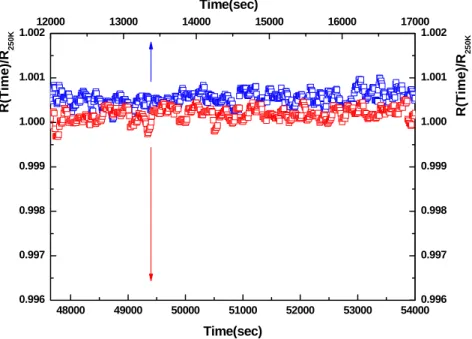
48000 49000 50000 51000 52000 53000 54000 0.996 0.997 0.998 0.999 1.000 1.001 1.002 12000 13000 14000 15000 16000 17000 0.996 0.997 0.998 0.999 1.000 1.001 1.002 Time(sec) R(T ime)/ R 250K R(Time)/R 250K Time(sec)
Fig.32 (b) This enlarged diagram reveals the constant value of the resistance before (blue open circles) and after (red open circles) a large applied H.
0 10000 20000 30000 40000 50000 0.0 0.2 0.4 0.6 0.8 1.0 0 25000 50000 75000 100000 R( T ime) /R 210K Time(sec) T= 210 K H(Oe )
Fig. 33 (a) At T = 210 K, after the largest drop of resistance with H = 9 tesla, the resistance still rejuvenated and kept the same value with time evolving, similar to the situation at T= 250 K.
12000 14000 16000 0.996 0.997 0.998 0.999 1.000 1.001 1.002 48000 50000 52000 54000 56000 0.996 0.997 0.998 0.999 1.000 1.001 1.002 R( Time)/ R21 0K R( Ti me )/R 21 0K Time(sec) Time(sec)
Fig. 33 (b) This enlarged diagram reveals the constant value of the resistance before (blue open circles) and after (red open circles) a large applied H.
Based on the data displayed in Fig. 32 and Fig. 33, the absence of resistance relaxation after the removal of the applied field, indicates that the system is in a single phase regime. In this sense the hysteresis of the electric transport properties described by the PS-model seems to require that there should be coexistence and competition between the
short-range CO phase and short-range FM phase for observing PMME. In order to further delineate the point, we carried out PMME experiments over a much wider temperature range (from 10 K to 190 K) instead of just in the hysteresis region (160 K < T < 180 K).
resistance relaxation behaves similarly as previously described. It is suggestive that even at this temperature where noticeable hysteresis is still quite vague the PS has started to emerge. The ratio of the resistance as a function of time (R(T)) and the resistance at T= 190 K was enlarged in fig. 34 (b) to reveal clearer view of relaxation tendency.
Fig. 35, Fig. 36 and Fig. 37 display the PMME in the hysteric region, which is supposed to have the most pronounced effect. As expected, the modulation of resistance was huge and clear with a comparably small Hth = 1000 Oe. The pronounced response to
a small perturbation of applied magnetic field, strongly suggest that in the hysterical region, the newly formed CO and FM phases are relative by vulnerable and a small perturbation can affect the competition between the phases.
Fig. 38, Fig.39 and Fig. 40, on the other hand, demonstrate the PMME in the LT region. In this region, generally CO phase and FM phase are both in long-range scale and are both more robust. The magnetic force must be stronger to disturb this metastable state. As we can see in table 3, the Hth at T=80 K is 2 tesla while the Hth at T= 50 K and
T= 10 K is 3 tesla. The magnitude order is same as at T = 190 K and one-order larger than Hth in the hysteresis region.
Above TCO Below TCO In the hysteresis
region
Low temperature region
Hth(Tesla) None None 2 0.1 0.1 0.1 2 3 3
Table 3. The Hth at all temperatures are listed. The Hmax applied at T= 210 K and T =
250 K was 9 tesla, and we still cannot find the PMME phenomena; therefore we cannot define Hth at these two temperatures.
0 10000 20000 30000 40000 50000 0.00 0.25 0.50 0.75 1.00 0 20000 40000 60000 T= 190 K H(Oe) R( Time)/R 190K Time(sec) Hth
Fig. 34 (a) The PMME experiment at T= 190 K. Notice the sudden drop of resistance accompanied with Hth.
23000 24000 25000 26000 27000 0.995 0.996 0.997 0.998 0.999 1.000 1.001 1.0020 1000 2000 3000 4000 5000 0.995 0.996 0.997 0.998 0.999 1.000 1.001 1.002 R(Time)/R 190K
Time(sec)
R(Time)/R 190KTime(sec)
Fig.34 (b) The enlarged plot clarifies the decreasing and increasing relaxation tendency. 0 10000 20000 30000 40000 50000 0 1000 2000 3000 4000 0 2000 4000 6000 8000 10000 T= 177 K H(Oe) R(ohm)
Time(sec)
H
th22000 23000 24000 25000 26000 1100 1105 1110 1115 1120 11000 12000 13000 14000 15000 16000 1708 1712 1716 1720 1724 1728 R(ohm) Time(sec) R(ohm) Time(sec)
Fig.35 (b) The enlarged plot demonstrates the decreasing and increasing relaxation tendency. 0 10000 20000 30000 40000 50000 0 2000 4000 6000 8000 10000 12000 0 2000 4000 6000 8000 10000 T= 174 K H(O e) R( o h m ) Time(sec) H in plnae Hth
22000 23000 24000 25000 26000 7560 7580 7600 7620 7640 11000 12000 13000 14000 15000 9520 9540 9560 9580 9600 9620 R( oh m) Time(sec) R(ohm) Time(sec)
Fig.36 (b) The enlarged plot demonstrates the decreasing and increasing relaxation tendency. 0 10000 20000 30000 40000 100 200 300 400 500 600 0 2000 4000 6000 8000 10000 H( Oe) R( o h m)
Time(sec)
H th T=167 K23000 24000 25000 26000 27000 302.4 302.8 303.2 303.6 12000 13000 14000 15000 16000 397.0 397.2 397.4 397.6 397.8 398.0 398.2 398.4 R(ohm) Time(sec) R( ohm) Time(sec)
Fig.37 (b) The enlarged plot demonstrates the decreasing and increasing relaxation tendency. 0 10000 20000 30000 40000 50000 10 12 14 16 18 20 22 0 20000 40000 60000 80000 100000 H(Oe ) R( ohm)
Time(sec)
T=80 KH
thFig.38 (a) The PMME experiment at T= 80 K. 11000 12000 13000 14000 15000 16000 19.90 19.95 20.00 20.05 20.10 0 1000 2000 3000 4000 21.0 21.2 21.4 R(oh m) Time(sec) R(oh m) Time(sec)
Fig.38 (b) The enlarged plot shows the decreasing and increasing relaxation tendency. 0 10000 20000 30000 40000 50000 9 10 11 12 13 14 15 160 20000 40000 60000 80000 R( o h m)
Time(sec)
H( Oe) T= 50 KH
thFig.39 (a) The PMME experiment at T= 50 K. 24000 26000 28000 12.85 12.90 12.95 13.00 13.05 13.100 1000 2000 3000 4000 5000 14.0 14.5 15.0 15.5 16.0 R(ohm) Time(sec) Time(sec) R(ohm)
Fig.39 (b) The enlarged plot demonstrates the decreasing and increasing relaxation tendency. 0 10000 20000 30000 40000 50000 60000 6 7 8 9 10 11 12 0 20000 40000 60000 80000 100000 H(T esla) R(ohm)
Time(sec)
H
th T=10 KFig.40 (a) The PMME experiment at T= 10 K. 24000 26000 28000 8.44 8.45 8.46 8.47 8.48 8.49 8.50 8.51 8.52 8.53 8.54 0 2000 4000 11.360 11.365 11.370 R(ohm) R(ohm) Time(sec) Time(sec)
Fig.40 (b) The enlarged plot clarifies the decreasing and increasing relaxation tendency.
c.Metastable Resistance-temperature (RT) dependence
After we conducted the PMME experiments at various temperatures, we could roughly decide the metastable resistance-temperature (RT) dependence. Fig. 41 illustrates the metastable RT dependence. Each data plotted in Fig.41 represents a single PMME
experiment at that temperature. Based on the data acquired from the PMME experiments, we could obtain Rmin, the minimum resistance from 90-minute relaxation after the
removal of H for H<Hth, and Rmax, the maximum resistance we obtained from 90-minute
relaxation after the removal of H for H>Hth. Rave denotes the arithmetic average of Rmax
T= 190 K. We further compare the obtained metastable RT dependence with that obtained from a “standard” R(T) measurement (Fig. 42). As is evident from the results, both values agree quite well, indicating that the current measurements are closely related to the usual transport measurements.
0 50 100 150 200 250 10 100 1000 10000 189.9 190.0 190.1 7224 7226 7228 7230 R(Ohm ) T(K)
Rmin after removal of H<Hth Rmax after removal of H>Hth RAve of Rmin& Rmax
Tco
Metastable R Single Phase R
Fig. 41 The diagram shows the single-phase RT dependence above TCO linked with a
black line; a green line indicates the metastable RT dependence.
0 50 100 150 200 250 300 10 100 1000 10000 0 50 100 10 15 20 25 30 35 40 R( Ohm) T(K) RAve of RMax&RMin normal RT
Fig. 42 The plot marks the metastable points of R(T) dependence by red crosses, comparing to that of a standard R(T) measurement. The inset reveals the disability of resistance rejuvenation at low temperatures.
To reconsider the above results obtained form the PMME experiments and the metastable RT dependence we suggest here a possible transport mechanism based on the PS model depicted schematically in Fig.43. This picture is consistent with the model proposed by M. Uehara et.al [14], in that emphasis has been focused on the short-range phases. In our case, the short-range phases depicted in Fig.43(a) dominate the transport behavior for temperature just below the TCO; Fig.43(b) illustrates the
distribution of the tow separated phases in the hysteresis region. For even lower temperatures the separatede phases become long range ordered phases and as depicted schematically in Fig.43(c). As our PMME results revealed at T= 190 K, the applied H did not affect the transport behavior very much because of the size and amount of the two phases and still too tiny to dominate the transport properties. On the other hand, PMME data in the hysteresis region indicated that a strong disturbance in resistance could be made with a small applied H, suggesting that not only the size and amount of the two phases become large enough to determine the transport properties but also they are susceptible to relatively lower field. Finally, for lower temperatures, an even larger H is needed for observing PMME. This can be understood since at these
temperatures the two separated phases are in long-range order regime and may become robust enough and are difficult to be disturbed by external fields.
Fig. 43 (a) Illustration of the two separated phases at temperature just below TCO to
indicate the CO and FM phases just start to grow and the sizes are small.
Fig.43 (b) Illustration of the two separated phases in the hysteresis region where the CO phases and FM phases are larger and compete with each other intensively.
Fig.43 (c) Illustration of the two separated phases at low temperature suggests the long-range CO and FM phases’ existence and the disturbance affect less in this region.
d.R-H Oscillation Experiments at Various Temperatures
To further depict the scenario proposed above, we conducted R-H oscillation
experiments at T=190 K (Fig.44, just below TCO), T= 174 K (Fig.45, in the hysteresis region),
and T= 130 K (Fig.46, at low temperature). These experiments were designed to use the oscillating field to “stir” the metastable state that will effectively remove the effect of Hthand
hence accelerate the relaxation. We first cooled the sample to the temperature aimed. Then, we applied a H which is larger than Hth,removed it, and measured the resistance relaxation
for 200 minutes. This is done in order to compare subsequently the behaviors under oscillating H the same period of time. Finally, we applied an descendent oscillating H and measured the change of the resistance simultaneously over the same period of time. The results measured at T= 190 K is shown in Fig. 44(a). In this case, both the zero-field
relaxation and oscillating field “stirred” relaxation display consistent behaviors with an increasing relaxation in R. Fig. 44(b) illustrates the R-H hysteresis loops upon the R-H oscillation. The fact that the size of each loop responding to the descending field remains essentially the same is indicative of a relatively undisturbed phase-separation distribution under such conditions. Since Hth (190 K) ~ 2 T I smuch larger over than the Hosc.(max)
applied here, we expect that the Hosc. applied here, though effectively changed the overall
resistance by maybe usual magnetoresistance behavior, does not alter the phase separation distribution and hence did not affect the resistance relaxation (or PMME). Fig. 45(a) shows the results at T= 174 K, revealing that the stirring of the applied oscillating field causes an even larger increase in resistance with time than the original zero-field relaxation over the same duration of time. Fig. 45(b) shows a distinctly different R(H) hysteresis at this regime. The larger hysteresis R(H) loops indicates even a small field can affect the transport behavior significantly. We believe that in this temperature regime, since the coexisting new phases start to play a more significant role in determing the transport properties and are not yet robust enough. Thus, the resistnace is susceptible to even a small field. However, at T = 130 K (as shown in Fig. 46(a) and 46(b)) even the applied field is as large as 3 Tesla, due to the
robustness of the long range ordered CO and FM phases, only very little hysteretic effects are discernible.
0 5000 10000 15000 20000 0.6 0.8 1.0 -10000 -5000 0 5000 10000 R(T )/ R1 90K Time(sec) H( O e ) T= 190 K
Fig.44(a) The red line represents the original increasing relaxation tendency. After the R-H oscillation, the resistance relaxation still follows the original tendency.
-10000 -5000 0 5000 10000 0.6 0.7 0.8 0.9 1.0 R(H )/ R 190K H(Oe) T= 190 K
0 5000 10000 15000 20000 0.0 0.2 0.4 0.6 0.8 1.0 1.2 1.4 -10000 -5000 0 5000 10000 R(T )/ R174 K Time(sec) H( O e ) T=174 K
Fig.45(a) The red line represents the original increasing relaxation tendency. After the R-H oscillation, the resistance relaxation tendency increased more than the original.
-10000 -5000 0 5000 10000 0.2 0.4 0.6 0.8 1.0 1.2 1.4 0 100 200 300 0 2 4 6 8 10 H(Oe) R(H)/ R174 K T= 174 K R(T) RAve of RMax&RMin
T(K)
Fig.45(b) The symmetric R-H hysteresis is clearer and larger with same H oscillation than that at T= 190 K.
0 5000 10000 15000 20000 0.6 0.8 1.0 1.2 -30000 -20000 -10000 0 10000 20000 30000 130K Time(sec) R(T)/R H( O e ) T=130 K
Fig.46(a) Fig.41(a) The red line represents the original increasing relaxation tendency. After the R-H oscillation, the resistance relaxation shows a slight decrease, comparing to the original tendency.
-30000 -20000 -10000 0 10000 20000 30000 0.80 0.85 0.90 0.95 1.00 R( H )/ R1 30K H(Oe) T= 130 K
Chap.5 Summary and Conclusions
In discussing the nature and consequences of the phase separation model, we propose a size-effective mechanism to relate the detailed distribution of the coexisting phases to the measured magneto-transport properties. By studying the time-relaxation of resistance at different temperatures, properties have been shown to intimately correlate the electric transport with competitions between the coexisting phases. In particular, we
demonstrated that, although the PMME phenomena can be discerned over a much wider temperature range than previously anticipated, the properties are most susceptible to external disturbances (e.g. temperature change or applied magnetic field) when it is in the vicinity of phase transition regime. Our experiments also demonstrated that both the amount and robustness of the CO phases may be playing the dominant role in giving rise to the R (T) hysteresis in LPCMO. This may also explain why the PMME is absent in LCMO system. Fig. 47 illustrates the different phase transitions with decreasing temperature in the two systems. The hysteretic and the relevant relaxation behaviors observed in this study could be due to two possibilities resulted from the formation of CO phase. One is the existence of CO-phase is the sole reason. The other is that the behavior may be general for phase coexistent systems; nevertheless, the relaxation process is too fast for the FM phase as compared to that of the CO phase. Thus, we only see the manifestations of the CO phase. Further work is certainly needed to discern these
proposed possibilities.
Fig. 47 A schematic illustration expresses the phase transition with decreasing
temperature in LCMO and LPCMO. PI denotes the paramagnetic insulator, FM denotes the ferromagnetic metal, and COI denotes the charge-ordering insulator.
References
[1]G.H. Jonker and J.H. van Santen, Physica 16, 337 (1950).
[2] G. C. Xiong, Q. Li, H. L. Ju, S. M. Bhagat, S. E. Lofland, R. L. Greene, and T. Venkatesan, Appl. Phys. Lett. 67, 3031 (1995).
[3]C.Zener, Phys. Rev. 82, 403 (1951).
[4]H.Y. Hwang , S-W Chenog, P.G. Radaelli, M.Marezio, and B.Batlogg, Phys. Rev. Lett. 75, 914 (1995).
[5]N. Mannella, A.Rosenhahn, C.H. Booth, S. Marchesini, B.S. Mun, S.-H. Yang, K. Ibrahim, Y. Tomioka, and C.S. Fadley, Phys. Rev. Lett. 92, 166401(2004).
[6]M. Jaime, M.B. Salamon, M. Rubinstein, R.E. Treece, J.S. Horwitz, and D.B. Chrisey, Phys. Rev. B 54, 11914(1996).
[7] O. Toulemonde, F. Studer, A. Barnabé, A. Maignan, C. Martin, B. Raveau, J. Phys. 11,109(1999).
[8]Jan Burgy, Adriana Moreo, and Elbio Dagotto, Phys. Rev. Lett. 92, 097202(2004). [9]F. Parisi, P.Levy, L.Ghivelder, G.Polla, and D. Vega, Phys. Rev. B 63,144419(2001). [10J.X. Ma, D.T. Gillaspie, E.W. Plummer, and J. Shen, Phys. Rev. Lett. 95, 237210(2005). [11]A.Masuno, T.Terashima, Y.Shimakawa, and M. Takano, Appl. Phys. Lett. 85, 6194(2004). [12] E.S. Vlakhov, K.A. Nenkov, T.I. Donchev, E.S. Mateev, R.A. Chakalov, A.Szewczyk,
[13]A. Moreo, Seiji Yunoki, and Elbio Dagotto, Science 283, 2034(1999). [14]M.Uehara, S.Mori, C.H. Chen and S.-W. Cheong, Nature 399, 560(1999).
[15]Liuwan Zhang, Casey Israel, Amlan Biswas, R.L.Greene, and Alex de Lozanne, Science 298, 805(2002).
[16]L. Ghivelder and F.Parisi, Phys. Rev. B 71, 184425(2005).
[17]M.tokunaga, Y.Tokunaga, and T.Tanegai, Phys. Rev. Lett. 93, 037203(2004).
[18]N.A. Babushkina, L.M. Belova, D.I. Khomskii, K.I.Kugel, O.Yu. Gorbenko, and A.R. Kaul, Phys. Rev. B 59, 6994(1999).
[19]S. Taran, Sandip Chatterjee, and B.K. Chaudhuri, Phys. Rev. B 69, 184413(2004). [20]A. S. Ogale, S.R.Shinde, V.N. Kulkarni, J.Higgins, R.J. Choudhary, Darshan C.
Kundaliya, T.Polleto, and S.B.Ogale, Phys. Rev. B 69, 235101(2004).
[21]M. Quintero, A.G.Leyva, P.Levy, F.Parisi, O.Aguero, I.Torriani, M.G. das Virgens, L.Ghivelder, Physica B 354, 63(2004).
[22]T. Wu, S.B. Ogale, S.R.Shinde, Amlan Biswas, T.Polletto, R.L.Greene, and A.J. Millis, J. Appl. Phys. 93, 5507(2003).
[23]P. Levy, F. Parisi, L. Granja, E. Indelicato, and G.Polla, Phys. Rev. Lett. 89, 137001(2002).
G.Gorodetsky, Phys. Rev. B 72, 134414(2005).
[25] P. Levy, F. Parisi, M. Quintero, L. Granja, J. Curiale, J. Sacanell, G. Leyva, and G. Polla, Phys. Rev. B 65, 140401(2002).
[26]D.D.Sarma, Dinesh Topwal, U.Manju, S.R. Krishnakumar, M.Bertolo, S.La Rosa, G.Cautero, T.Y. Koo, P.A. Sharma, S.-W. Cheong, and A. Fujimori, Phys. Rev. Lett. 93, 097202(2004).
[27]A. J. Millis, P. B. Littlewood, and B. I. Shraiman, Phys. Rev. Lett. 74, 5144(1995). [28]J.M. De Teresa, M.R. Ibarra, P.A. Algarabel, C.Ritter, C.Marquina, J.Blasco, J.Garcia,
A.del Moral, and Z.Arnold, Nature 386, 256(1997). [29]Y.Tokura and N. Nagaosa, Science 288, 462(2000)
[30]simple interpretation could be found in Introduction to Solid State Physics, C. Kittel, 1953 [31]T. Tomioka and Y. Tokura, Phys. Rev. B 70, 014432(2004).
[32]S. Dong, Han Zhu, X.Wu, and J.-M. Liu, Appl. Phys. Lett. 86, 022501(2005). [33]E. Dagotto, Science 309, 257(2005).
[34]STM image provided by W.J. Chang, department of electrophysics, National Chiao Tung University, Taiwan
[35] These figures are illustrated by Matthias Mayi
[39]J.Y. Lin, C.W. Chen, Y.C. Liu, S.J. Liu, K.H. Wu, Y.S. Gou, and J.M. Chen, J. Mag. Mag Mate. 239, 48(2002).
Phys. Rev. B 40, 5715(1989).
[41]H.L. Ju, H.-C.Sohn, and Kannan M. Krishnan, Phys. Rev. Lett. 79, 3230(1997).
[42]G.M. Zhao, V.Smolyaninova, W. Prellier, and H.Keller, Phys. Rev. Lett. 84, 6086(2000). [43]H. Eskes, M.B.J. Meinders, and G.A. Sawatzky, Phys. Rev. Lett. 67, 1035(1991).
[44]J.H. Park, C.T. Chen, S-W. Cheong, W.Bao, G.Meigs, V.Chakarian, and Y.U. Idzerda, Phys. Rev. Lett. 76, 4215(1996).