國 立 交 通 大 學
資訊科學與工程研究所
碩士論文
解交錯演算法使用平滑條件適應性選擇
空間與時間的插補
A De-interlacing Algorithm Using
Smoothness Constraint for Adaptive
Spatiotemporal Interpolations
研究生 :陳敏正
指導教授:彭文孝 教授
解交錯演算法使用平滑條件適應性選擇
空間與時間的插補
指導教授 : 彭文孝 教授
學生:陳敏正
國立交通大學
資訊科學與工程研究所
新竹市大學路 1001 號
2008 年 9 月
摘要
本論文中,我們呈現一個動態選擇空間插補與動態補償的混和式
的解交錯演算法。在空間插補的演算法中,我們參考了影像補償的觀
念,等光線,估計出大約的平滑方向且在稍後的步驟中正確的找出與
粗估的最相近的方向。時間插補方法中,動態補償是主要的時間插補
的結果。在動作估計中,我們增加一個平滑限制的因子使得由動作估
計呈現出動作向量的連續性而且也會產生出較好的動態補償結果。
為了避免因為錯誤動作向量所產生的嚴重區塊失真,利用動作向
量能量與自相關函數去偵測哪一個向量是否是錯誤的。像素值應該與
其相鄰的像素有關連性是眾所周知的。把像素基礎的亮度的關聯性轉
換成以區塊基礎的動作向量,我們引用了兩種不連續的類型去估計動
作向量的能量:區域與上下文的不連續。一般而言,大的動作向量能
量值越大表示此向量越不可靠。
在我們的方法中,大量的平滑邊與區塊失真都被正確的找出。選
擇插補的方法依靠動作資訊而不採用空間特性且最後的輸出是空間
與時間插補的二分選擇。實驗的 PSNR 數據比現有新穎的演算法至少
有 0.5db 的增加。
A De-interlacing Algorithm
Using Smooth Constraints
for Adaptive Spatiotemporal Interpolations
Advisor: Prof. Wen-Hsiao Peng
Student: Ming-Chang Chen
Institute of Computer Science and Engineering
College of Computer Science
National Chiao Tung University
1001 Ta-Hsueh Rd., 30010 HsinChu, Taiwan
Abstract
In this thesis, we present a hybrid de-interlacing algorithm using spatial interpo-lation and motion compensation. The spatial interpointerpo-lation refers to the concept of image inpainting, isophote, to estimate smooth direction approximately and then corrected by smoothness factor further. In temporal interpolation, motion com-pensation (MC) is the major temporal result. In the motion estimation (ME), we add a factor of smoothness constraint to present the continuity of motion vector (MV) and it would produce better motion compensated result.
In order to prevent the signi…cant block e¤ect caused from erroneous MV, using the energy of MV and autocorrelation function to detect which MV(s) is erroneous. It is well known that pixel value has correlation with its nighborhoods. To translate the correlation from pixel-based intensity value to block-based MV length, we introduce the two types of discontinuity on MV to evaluate the motion vector energy (MVE) of MV: local and contextual discontinuity. Generally, the large measure score of MVE means that the MV is unreliable, vice versa.
The signi…cant smooth edges in spatial method and block artifacts in temporal results are recognized correctly. The manner of choosing interpolation depends on the motion information rather than spatial feature and the …nal output is a binary decision between spatial and temporal interpolation. The simulated peak signal-to-noise ratio (PSNR) of proposed algorithm have at least 0.5dB better than other novel de-interlacing algorithms.
誌謝
我在這裡要感謝我的指導教授 彭文孝教授,兩年來對我孜孜不倦的
教誨,教導我研究學問的方法與分析,讓我畢生受益無窮,以及我的
口試委員 林嘉文教授 與 蕭旭峯教授,二位老師不吝指教,讓這篇
論文更加完善。
我還要感謝李志鴻學長、陳渏紋學長與林鴻志學長,給予我論文研究
及寫作方面等的各種建議,感謝同學黃雪婷、林岳進、與學弟陳俊吉、
陳建穎、林哲永與詹家欣,在這兩年內與我共同努力,互相砥礪,陪
我度過這段快樂的實驗室生活。
僅將此論文獻給我親愛的家人與朋友,我的父母及朋友,感謝他們在
這段期間給我的關心、支持與鼓勵,祝福他們永遠健康快樂。
陳敏正 謹誌於 國立交通大學資訊科學與工程研究所 中華民國九十七年九月Contents
Contents 1 List of Tables 4 List of Figures 5 1 Introduction 1 1.1 Background . . . 1 1.2 Motivation . . . 4 1.3 Thesis Organization . . . 4 2 Review of Prior Works 5 2.1 Spatial Interpolation . . . 6 2.1.1 Line Doubling . . . 62.1.2 Linear Average Interpolation . . . 6
2.1.3 Edge-based Linear Average (ELA) . . . 7
2.2 Temporal Interpolation . . . 9
2.2.1 Motion Adaptive Approach . . . 10
2.2.2 Motion Compensated Approach . . . 15
2.2.3 Four-…eld Motion Compensation . . . 16
2.2.4 Erroneous Motion Vector Protection Strategy . . . 17
3 Proposed De-interlacing Algorithm 20 3.1 Spatial Interpolation . . . 20
3.1.1 Isophote Interpolation . . . 21
3.1.2 Adaptive Decision of Dominant Edge . . . 25
3.2 Proposed Motion Compensated Interpolation . . . 26
3.2.1 Vertical Even-step of MV Search Window . . . 26
3.2.2 Match Criterion with Smoothness Constraint . . . 28
3.3 Proposed MV Protection Strategy . . . 30
3.3.1 Motion Vector Reliability (MVR) Problem . . . 30
3.3.2 MV Local Discontinuity . . . 30
3.3.3 MV Contextual Discontinuity . . . 31
3.3.4 Irregular and Regular MVs . . . 33
3.3.5 Autocorrelation Detection . . . 36
3.3.6 Stationary Pixel Detection and Output Decision . . . 38
4 Experimental Results and Analysis 39 4.1 Analysis of MV Smoothness Constraint . . . 39
4.2 Analysis of Reliable and Unreliable Blocks . . . 42
5 Summary and Conclusion 56 5.1 Summary . . . 56 5.2 Conclusion . . . 57 5.3 Future Work . . . 58
List of Tables
4.1 The testing parameters. . . 40 4.2 Table of PSNR Comparison. . . 51
List of Figures
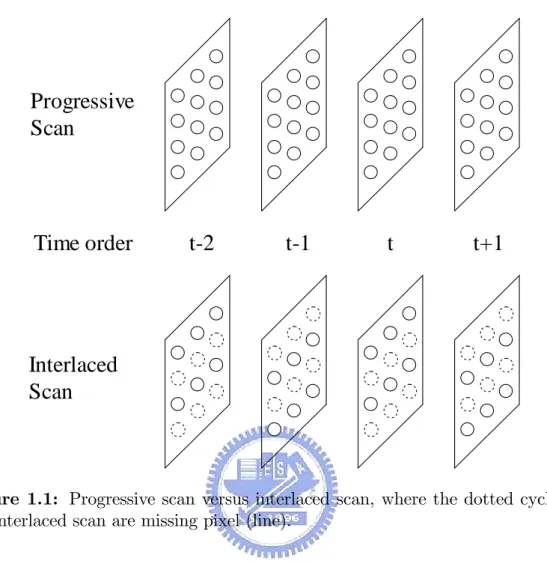
1.1 Progressive scan versus interlaced scan, where the dotted cycles in
the interlaced scan are missing pixel (line). . . 2
2.1 Line doubling scheme. . . 6
2.2 Bob method. . . 7
2.3 Edge-based line average. . . 8
2.4 Block-based ELA. . . 8
2.5 Direction-oriented interpolation. . . 10
2.6 The visual artifacts of de-interlacing in (a) the fast motion region, (b) the occlusion region, and (c) the region with scene change. . . . 11
2.7 Three-…eld motion detection. . . 12
2.8 Four-…eld motion detection. . . 12
2.10 (a) Cross-shaped window. (b) Combinations of di¤erence pairs. . . 13
2.11 Five-…eld motion detection. . . 14
2.12 Four-…eld motion estimation. . . 16
2.13 Neighborhood system of a block. . . 18
3.1 Proposed de-interlacing structure. . . 21
3.2 Prewitt mask in proposed spatial method. . . 22
3.3 The graident vector …eld (grad_v; grad_h) and corresponding isophote vector …eld (iso_v; iso_h). . . 23
3.4 De…ned neighboring structure of interpolated pixel. . . 23
3.5 Visual artifacts of de-interplacing by merely performing spatial In-terpolation along the isophote direction. . . 24
3.6 Subjective quality of the de-interplaced images using the smooth-ness constraint. . . 25
3.7 Comparison of (a) odd-valued and (b) even-valued vertical displace-ments. . . 27
3.8 Estimated motion vector M V (x; y) and its …ve neighbors located at spatial and temporal respectively. . . 29
3.9 (a) MC only picture, (b) After true motion detection. . . 32
3.10 Result of true motion and MVE detection. . . 33
3.11 (a) MC picture at 190th frame in foreman sequence, (b)MVE dis-tribution relative to (a). . . 34
3.12 (a) Good MC picture in coastguard sequence. (b) False detection caused by irregular MVs surrounding. (c) Neighboring MVs of cur-rent MV in (b). . . 34
3.13 Periodic wave in sequence of autocovariance values. . . 37
4.1 The in‡uence of Landa MV for sequences. (a) Foreman. (b) Stefan. (c) Coastguard. (d) Container. . . 41 4.2 Artifact caused by large landa (a) Occlusion area, the foreman’s
tongue. (b) Fast motion. . . 42 4.3 Total number of unreliable blocks entire sequence. . . 43 4.4 Total number of unreliable blocks entire sequence with column-wise
autocorrelation. . . 44 4.5 Test ‡ow. . . 45 4.6 The experimental result for sequence "Foreman", "Bus." (a) Isophote
interpolation. (b) Motion Compensation. (c) Hybrid. . . 46 4.7 The experiment result for sequence "Aikyo", "Coastgurad."(a) Isophote
interpolation. (b) Motion Compensation. (c) Hybrid. . . 47 4.8 The experiment result for sequence "Mobile", "Container."(a) Isophote
interpolation. (b) Motion Compensation. (c) Hybrid. . . 48 4.9 The experiment result for sequence "Table", "Stefan." (a) Isophote
interpolation. (b) Motion Compensation. (c) Hybrid. . . 49 4.10 The experiment result for sequence "Silent", "Dancer." (a) Isophote
interpolation. (b) Motion Compensation. (c) Hybrid. . . 50 4.11 Bar chart of PSNR comparison. . . 51 4.12 The comparison of experimental result for sequence "Foreman",
"Bus" and "Table." (a) STCAD results in left column. (b) Pro-posed de-interlacer results in right column. . . 52 4.13 The comparison of experimental result for sequence "Dancer",
"Coast-guard" and "Container." (a) STCAD results in left column. (b) Proposed de-interlacer results in right column. . . 53
4.14 The missing detections in proposed algorithm. (a) Block artifacts of proposed algorithm in left column. (b) Better results of STCAD in right column. . . 54 4.15 The fasle detections in proposed algorithm. (a) Blurred image of
proposed algorithm in left column. (b) Better results of STCAD in right column. . . 55
CHAPTER 1
Introduction
1.1
Background
In modern of television system and display devices, there are two major scanning formats, interlaced scan and progressive scan, for di¤erent applications or client display devices. Progressive scan, scans all the lines of image and produces the picture data which called frame, and a collection of serious frame forms frame sequence. Interlaced scan scans either even-indexed or odd-indexed lines of image only and produces the picture data which called …eld. The popular standard of …eld sequence stands for a collection of successive …elds, even-indexed and odd-indexed …elds are sorted alternately in display order. In general, the frame sequence is original sequence for display, and the …eld sequence is down-sampled from frame
t
t-1
t-2
t+1
Progressive
Scan
Interlaced
Scan
Time order
Figure 1.1: Progressive scan versus interlaced scan, where the dotted cycles in the interlaced scan are missing pixel (line).
sequence, as shown in Figure 1.1.
De-interlacing is the process to convert …eld sequence into frame sequence. Because of the limitation for some speci…ed applications or bandwidth of trans-mission environments, the …eld sequence conversion is necessary for progressive display devices. Digital display devices, for example, digital TV and multimedia PC, support display of frame sequence while traditional analog TV supports dis-play of …eld sequence. If …eld sequence have to be disdis-played on digital disdis-play devices, the de-interlacing is required for converting the …eld sequence into frame sequence. The de-interlacing is also a frame rate up-conversion problem since
the scene is unreconstructable when the sample rate is insu¢ cient. For exam-ple, there are two di¤erent frame rate sequences, 30 frames/sec and 60 …elds/sec, which would like to be converted into 60 frames/sec. The converted result of 30 frames/sec could be less performance than the result of 60 …elds/sec. According to the reason, de-interlacing is a better choice than other frame rate conversion approaches.
In [7], a review of currently available de-interlacing algorithms was shown and categorized into two classes, motion compensated (non-MC) de-interlacing and MC de-interlacing [16]. The Non-MC de-interlacing algorithms involve several de-interlacing methods, line doubling , linear average (Bob) and edge-based lin-ear average, which are classi…ed into spatial methods in this thesis. The line doubling and Bob method are typical and simple approaches for spatial interpo-lation; however, they would casue some problems to annoy human vision, like ‡icking and sawing edge. Because of the drawbacks of typical spatial methods, the edge-base method have been developed [8][24][1] to …x it. Those methods perform well in stationary image, but less e¤ective with texture image. There-fore, the motion adaptively (MA) methods were invented to reduce such problems [12][13][18][19][22][25]. Although the MA methods are able to reduce such prob-lem, but it is not complete because useful in stationary area only. Hence, the MC de-interlacing algorithms were suggested for motion object, and perform well without in‡uence of spatial feature, given accurate motion information. It is well know that the direct MC algorithm is sensitive to motion vector. The signi…cant artifacts are occurring when the relative motion vector is erroneous. According to the reason, the MV protection strategies were introduced against the erroneous MVs [16][17][20][21][23]. It is our research objective to banish the signi…cant block artifacts from MC de-interlacing algorithm.
1.2
Motivation
Because the MC algorithm can provide the better interpolated result than non-MC algorithm does, our approach tends to use the great quantity of motion compensated results as major output of proposed de-interlacing algorithm. Conse-quently, an e¢ cient MC de-interlacer has to include e¤ective protection strategies, which can protect the de-interlacer’s performance against incorrect MVs. In [16] and [23], the authors have suggested MV protection strategy in order to against the serious block artifacts caused by erroneous MVs. In study of [16] and [23], we discover that both methods have a common feature in MV protection strat-egy, spatial image feature. Using spatial image feature is not robust enough for determining which MV(s) is erroneous because it may be failed in some of special cases, for horizontal edge, texture image and multi-edge area. In order to avoid the weakness of spatial feature, our approach discards the analysis of spatial feature then takes all motion information into account to analyze and determine erroneous MVs.
1.3
Thesis Organization
The outline of the paper is as follows. In chapter 2, we review several the most common de-interlacing approaches and discuss the issues brie‡y. In chapter 3, we explain the main idea of our proposed de-interlacing algorithm, including isophote interpolation, modi…ed motion estimation and MV protection strategy. In chapter 4, we will show the analysis of problems we met, and the performance of proposed de-interlacing algorithm for comparing with other de-interlacing algorithms. The …nal chapter summarizes the proposed methods respectively, and describes some of problems occurred in proposed algorithm.
CHAPTER 2
Review of Prior Works
This chapter is devoted to discussing some of the methods in available de-interlacing approaches proposed early and their problems. Those de-de-interlacing approaches can be divided into temporal and spatial methods. These methods can be complicated or easy to implement for di¤erent applications. All of the de-interlacing methods have the same goal, that is, to interpolate the missing …eld data to reconstruct the complete frame. In this thesis, we classify the de-interlacing methods into three categories: spatial method, temporal method, and hybrid method. We will describe these methods brie‡y and discover which problem could be.
Before entering the …rst section, to …x the notations are necessary. ft; bft :Original and reconstructed …eld at time t; respectively.
Original pixel line
Original pixel line Missing pixel line 0 -1 -2 1 2 0 1 -1
Figure 2.1: Line doubling scheme.
I(x; y) : Intensity value of pixel site (x; y) with respect to the frame coordi-nate.
4I(x;y) :Intensity variation with respect to the frame coordinate.
2.1
Spatial Interpolation
2.1.1
Line Doubling
This method is de…nitely a fundamental technique in available de-interlacing scheme, which has lowest complexity because it simply replace the missing line with upper vertical existent line. The Figure 2.1 illustrates the method of line doubling and corresponding equation, which is Eq. 2.1.
It(x; y) = It(x 1; y) (2.1)
The line doubling method is very easy to implement but it may cause ‡ickering e¤ect in temporal visual and saw e¤ect on the edge of object.
2.1.2
Linear Average Interpolation
Each missing pixel is interpolated by averaging the two original pixels which are located at upper and lower sites of interpolated pixel. This method is called
... ... ... ... y x x-1 x+1 y-1
y+2 y+1 y+2
...
Figure 2.2: Bob method.
“Bob” method. The common equation (Eq. 2.2) can be expressed as follows: It(x; y) =
1
2[It(x 1; y) + It(x + 1; y)] (2.2) Figure 2.2 illustrates the Bob method of interpolation. That is suitable for real time application like digital display because of its low calculation. Although the Bob method is a low complexity method of calculation, it will cause the line ‡ickering along edge in display.
2.1.3
Edge-based Linear Average (ELA)
The ELA method is the most popular method in the available de-interlacing methods, and it have been employed in many other spatial-based algorithms [7]. These methods try to use the edge information present in the scene for recovering the interpolated pixel properly. Therefore, the key point of those interpolation methods is to determine the smoothest direction correctly for the interpolated pixel. The missing pixel value is produced by linearly averaging the pair of pixels according to the determined edge. In [8], if (x; y) is the pixel to interpolate, the edge information is estimated by evaluating three pixel di¤erences in the 3x3 block centered around it. These three pixel di¤erences jIt(x 1; y 1) It(x + 1; y + 1)j,
x x-1
x+1
y y+1 y-1
Figure 2.3: Edge-based line average.
y y+1 y+2 y+3 y+4 y-1 y-2 y-3 y-4 x x-1 x-3 x+1 x+3 Er El
Figure 2.4: Block-based ELA.
in Figure 2.3. The pixel (x; y) is then linearly averaged between the pair of pixels that result in the minimal pixel di¤erence.
Some of the ELA-enhanced algorithms have been proposed. These methods of directional interpolation are stated as follows.
Block-based ELA [3]: In [3], the author suggested a block-based structure to determine best edge focus on interpolated pixel, as shown in Figure 2.4, where Er and El denote the de…ned right-side and left-side edge in the block
structure. The decision of edge is divided into three phases. The …rst phase …nds the minimal intensity di¤erence over all de…ned edges in the block structure, then determines if the direction is right or left. Second, suppose the found edge is right side Er, take the follow equation to check the founded
direction is dominant edge or not.
jI (Er) I(Rli)j < , i for all directions in left side (2.3)
where is a given threshold which tends to range from 10 to 30, which checks if Eris dominant edge or not. Final phase, the interpolated pixel is produced
by averaging two pixels alone the dominant edge.
Direction-oriented Interpolation [24] (DOI): This approach tries to determine the dominant edge at a missing pixel in a more robust method than the fundamental ELA method. For that purpose, instead of computing the pixel di¤erence along a direction to estimate the edge orientation, three blocks structures are centered at interpolated pixel are used. As shown in Figure 2.5, three blocks are used: mid block W0 is centered at the interpolated pixel
which contains upper reference line U0and lower reference line L0, and upper
block W1 and lower block W2 which contain the upper reference lines and
lower reference lines U0, U1, L0 and L1 respectively. By comparing the pixels
of W0 and W1, and the pixels of W0 and W2, thus, the edge direction can
be determined and interpolation is linearly averaged alone that edge.
2.2
Temporal Interpolation
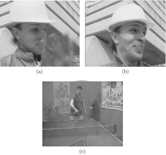
The major distinction between spatial and temporal interpolation is that the temporal method takes the pixel value to interpolate the missing pixel from the neighboring …eld in chronological. Generally, the temporal method results in the best interpolation result for objective measurement and subjective quality given accurate temporal information. On the contrary, the signi…cantly-annoying artifact is produced by erroneous temporal information than spatial method does. That annoying artifact often happens on the motion object, occlusion region, and scene
U0 U1 L0 L1 W0 W1 W2
Figure 2.5: Direction-oriented interpolation.
change, like Figure 2.6.
To discard those annoying artifacts and preserve the good result is the major objectives of this thesis.
2.2.1
Motion Adaptive Approach
In this thesis, the motion adaptive (MA) method [12][14][15][19][25] is categorized into temporal interpolation methods but it also uses the spatial interpolation to combine the advantages of both. Both interpolation methods are independent. The temporal information of MA method focuses on the site of interpolated pixel without any motion, where would be labeled as stationary or static pixel, which is decided by Eq. 2.4.
4I(x;y) =jIt 1(x; y) It+1(x; y)j (2.4)
First, de…ning a small and positive threshold value T HM A. If the value of
(a) (b)
(c)
Figure 2.6: The visual artifacts of de-interlacing in (a) the fast motion region, (b) the occlusion region, and (c) the region with scene change.
t-1 t t+1 x x+1 x+2 x-1 x
Figure 2.7: Three-…eld motion detection.
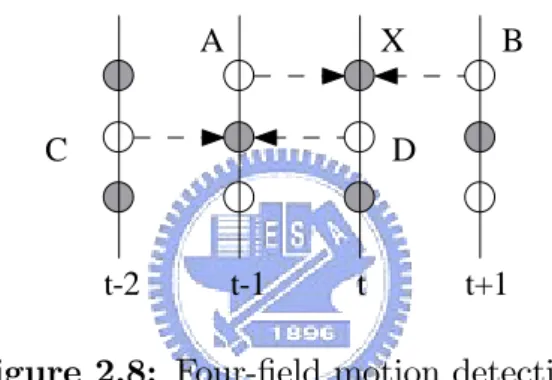
A B C D t t+1 t-1 t-2 X
Figure 2.8: Four-…eld motion detection.
as stationary. If the site of interpolated pixel was labeled as stationary, the recon-structed pixel value comes from the two nearest opposite parity …elds by averaging these pixels at same pixel coordinate, like Figure 2.7.
By employing the Eq.2.4, many stationary detection methods have been pro-posed for correctness of detection like four-…eld motion detection.
Four-…eld motion detection [19]: For illustrating four-…eld motion detection conveniently in Figure 2.8, using these symbols X, A, B, C and D denote the samples of intensity value to detect motion for pixel X at di¤erent time instance. The pixel X is static when both magnitudes of pixel di¤erence
A B C E D F G H I J X
Figure 2.9: Cross-shape motion detection.
|A-B|
|E-H|
|F-I|
|G-J|
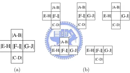
|C-D| |A-B| |E-H||F-I| |C-D| |A-B| |F-I||G-J| |C-D| |A-B| |E-H| |G-J| |C-D| |A-B||E-H||F-I||G-J| |E-H||F-I||G-J|
|C-D|
(a) (b)
Figure 2.10: (a) Cross-shaped window. (b) Combinations of di¤erence pairs.
jA-Bj and jC-Dj are small than T HM A.
Cross-shape window motion detection [13]: That is another motion detection called “cross-shape” window, which is shown in Figure 2.9. Next, a re…ning phase has to be considered to prevent erroneous motion state and calculating the summations of pixel di¤erence for all di¤erent combinations in Figure 2.10.
x x+1 x-1 t t-1 t+1 t+2 t-2
Figure 2.11: Five-…eld motion detection.
If any summation of pixel di¤erences is smaller than the de…ned threshold value, the pixel X is recognized as stationary. If the magnitudes of each pixel pair in the Figure2.9 are small than T HM A, the pixel X is detected as static
pixel.
Five-…eld motion detection [25]: This motion detection takes account of …ve …elds for estimating the motion of interpolated pixel. There are three pairs of pixel di¤erence for evaluating the motion state, shown in Figure 2.11. For simplicity, the motion activity P , Q and R are calculated respectively as Eq 2.5. P =jIt(x 1; y) + It(x + 1; y) 2 It 2(x 1; y) + It 2(x + 1; y) 2 j (2.5) Q =jIt(x 1; y) + It(x + 1; y) 2 It+2(x 1; y) + It+2(x + 1; y) 2 j (2.6) R =jIt 1(x; y) It+1(x; y)j (2.7)
the motion state ST of interpolated pixel is de…ne as follows
ST = max(P; Q; R) (2.8) If ST exceeds the T HM A, the motion activity is considered as static motion.
2.2.2
Motion Compensated Approach
The motion compensated approaches [3][4][9][11] perform well not only in sta-tionary areas but also moving objects, given accurate motion information. Because of the accurate motion information the motion compensated approach produces the best interpolated results than the other non-MC de-interlacing approaches. The motion compensated approach is sensitive to motion vector because the erroneous motion vector would cause conspicuous block artifact and make the subjective quality corrupt. The two problems of motion estimation would happen in both video coding and de-interlacing but cause di¤erent processed output.
The procedure of motion estimation in video coding is a pre-procedure to process image data before transmission; however, the procedure of motion esti-mation in de-interlacing is a post-procedure to process received image signals. The erroneous motion vector would cause signi…cant block e¤ect. In video cod-ing, such image e¤ect can be reconstructed completely by encoded residual image; however, there are no residual data could be employed for recovering the destroyed image caused by erroneous motion vector in de-interlacing. To conclude the motion estimation in the video coding, it may not corrupt image but in de-interlacing.
The other one is that the motion compensation process can not compensate odd-indexed missing line into even-indexed …eld along motion trajectory from motion estimation reference directly. The reference of motion estimation in de-interlacing should be same parity (even-indexed …eld to even-indexed …eld) as processing …eld is, but the source of compensation must come from the nearest …elds with opposite parity relative to current …eld.
In addition, an odd integer pixel displacement between successive …elds also makes such an artifact. Therefore, as the two problems mentioned above, serious artifacts could happen in motion compensation process. How to detect and prevent such errors would be considered later.
t
t+1
t-1
t-2
Search Window
mv block map in
same parity field
back-backward
backward
current
forward
MV
1/2MV
-1/2MV
Figure 2.12: Four-…eld motion estimation.
2.2.3
Four-…eld Motion Compensation
Chang et al. in [3][4] suggested a bidirectional motion compensated approach, in which the motion estimation denotes the …eld at time t 2 as back-backward …eld, the …eld at time t 1as backward …eld, current processing …eld at time t as current …eld, and the …eld at time t + 1 as forward …eld, motion estimation structure as following Figure 2.12:
This method also suggested a matching criterion SAD as following equation: SAD1j = P w2 jIt(xw + M Vxj;yw + M Vyj) It 2(xw M Vxj; yw M Vyj)j (2.9) SAD2j = P w2 jIt(xw+ 1 2M Vxj;yw+ 1 2M Vyj) It 2(xw 1 2M Vxj; yw 1 2M Vyj)j (2.10) where It(x; y)denotes the intensity value at the pixel site (x; y) of …eld with t time
set in search window with index j. Then the best candidate of displacement set is determined by minimizing the value of (SAD1j+SAD2j), which is
(M Vx; M Vy) = arg min
j [SAD1j+ SAD2j] (2.11)
The following phase is that compensate the interpolated pixel over trajectory from the two …elds backward …eld ft 1and forward …eld ft+1. The trajectory is set
to be 12M V and 12M V in Figure 2.12. The compensated block data indicated by
1
2M V is translated forward from backward …eld ft 1 and the compensated block
data indicated by 12M V is translated backward from forward …eld ft+1. After the
data transmission average these two data blocks as result of motion compensation. In this four-…eld MC method, the author also suggested a method of MV protection to detect block artifact “Feather e¤ect”, we will discuss it next section.
2.2.4
Erroneous Motion Vector Protection Strategy
In order to against the signi…cant block artifact introduced by erroneous mo-tion vector or absence of corrective compensated image data in neighboring …elds. There are many available methods of reliable motion detection have been proposed [7][10][16][17][21][23]. The problem is that the identi…cation of erroneous motion vector and the preservation of the reliable motion vector correctly. However, the motion vectors entire image should not be over-protected, which could limit the advantages of motion compensation and performance of de-interlacer.
There are lot of algorithms had discussed the linear combination of spatial and temporal interpolation, like equation as follows:
p^Is + (1 p)^It (2.12) where factor p is the proportion of spatial or temporal result handle the output
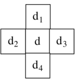
d
1d
2d
d
3d
4Figure 2.13: Neighborhood system of a block.
of de-interlacing. The linear combination of factor p is decided by how closely the two vertical neighbor pixels according to motion vector [7]. But the derivation of pis not obvious and not robust because it is hard to consider all features of image if calculated based on spatial information, for example, thin edge area.
The reliable MV detection [23] employ Gaussian white noise and Gibbs distri-bution to estimated the conditional probability and priori probability respectively. The posteriori probability of motion vector d(x; y) can be calculated by Bayes theorem and given assumptions of probability distribution. According to Bayes theorem, the posteriori probability formulate the equation, which is
P (djfk 1; fk) =
P (fkjd; fk 1)P (djfk 1)
P (fkjfk 1)
(2.13) where d , fk 1, and fk are denoted as displacement, prior and current …elds in
dis-play order respectively. P (fkjd; fk 1)is a conditional probability which is
approxi-mated base on the assumption that Gaussian White Noise, P (djfk 1)is considered
as Gibbs distribution to estimate priori probability, P (fkjfk 1) be replaced by a
constant because it is not a function of d.
P (djfk 1; fk) = expf 1 2 2 X x2 [fk(x) fk 1(x + d)]2g (2.14)
P (djfk) = expf U(djfk 1)g (2.15) U (djfk 1) = 1 2 2 d minfkd di k2 j0 < i 4g (2.16)
where is the set of pixel sites in block, in which 2
d is the variance of fk(x)
fk 1(x+d). U is the energy function, in which is the variance of d di(Figure 2.13)
among the neighbor block of current block. Finally the posteriori probability of conditional probability P (fkjfk 1; fk) can be expressed with above equations and
normalized factor C as follows: P (djfk 1; fk) = 1 Cexpf U(djfk 1) 1 2 2 X x2 [fk(x) fk 1(x + d)]2g (2.17)
The probability of reliability of processing MV is dominant using linear decrease function to decide if the length of MV is smaller than a prede…ned threshold or not.
CHAPTER 3
Proposed De-interlacing Algorithm
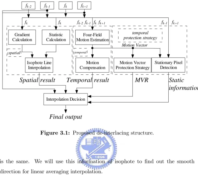
In our proposed algorithm, there are two interpolation units and two detector units in our de-interlacing structure, shows in Figure 3.1. Two units of interpola-tion are isophote-interpolated method and mointerpola-tion compensainterpola-tion respectively. The MV protection strategy and stationary pixel detection are employed for calculating temporal information. In the term of temporal information in proposed algorithm are motion vector energy (MVE) and stationary pixel respectively. The last part of structure is output decision to determine the interpolation is suitable for output.
3.1
Spatial Interpolation
In our proposed spatial method, we introduce a concept of Image Inpainting processing [2], isophote, it means that the level of intensity of pixels on the direction
Four-Field Motion Estimation Motion Compensation Isophote Line Interpolation Statistic Calculation Gradient Calculation Motion Vector Protection Strategy Interpolation Decision Stationary Pixel Detection fk-1 fk-2 fk fk+1 fk-1 fk fk+1 fk-2 fk-1 fk+1 fk fk spatial temporal Motion Vector temporal protection strategy
Final output
Spatial result
Temporal result
MVR
Static
information
Figure 3.1: Proposed de-interlacing structure.
is the same. We will use this information of isophote to …nd out the smooth direction for linear averaging interpolation.
3.1.1
Isophote Interpolation
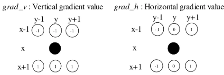
In image inpainting techniques [2], there is an important concept of image smoothing feature called “Isophote,” a direction where indicates the pixels along direction has same level of pixel value. To estimate the isophote direction, the gradient value is taken account. To conveniently calculate gradient value, Prewitt cross-gradient operator Figure 3.2 is taken and forms the gradient vector …eld (GVF) with respect to vector variable (grad_v; grad_h). It is well know that GVF represents the varying direction for the position of pixel in an image. On
-1 -1 -1 1 1 1 x-1 x x+1 y-1 y y+1
grad_v: Vertical gradient value
- 1 1 -1 0 1 y-1 y y+1 x-1 x x+1
grad_h: Horizontal gradient value
0
Figure 3.2: Prewitt mask in proposed spatial method.
the other hand, the normal of GVF can be represented as smooth direction for the position of pixel, that is so called "isophote" [2], which are illustrated in Figure 3.3. grad_v = It(x + 1; y 1) + It(x + 1; y) + It(x + 1; y + 1) 3 It(x 1; y 1) It(x 1; y) It(x 1; y + 1) 3 (3.1) grad_h = It(x + 1; y + 1) + It(x 1; y + 1) 2 It(x + 1; y 1) It(x 1; y 1) 2 (3.2)
The normal of GVF (grad _v; grad _h) forms the isophote vector …eld (IVF) (iso_v; iso_h), which is formed by replacing the gradient …eld reciprocally and make one of component negative, which is .
(iso_v; iso_h) = ( grad_h; grad _v) (3.3) After calculating of IVF, apply its information to prede…ned neighbor pixel
Gradient vector field (grad_v, grad_h)
Isophote vector field (iso_v, iso_h)
Figure 3.3: The graident vector …eld (grad_v; grad_h) and corresponding isophote vector …eld (iso_v; iso_h).
0 1 2 3 4 5 6 7 8 9 10
11 : missing pixel, preinterpolated. : existent pixel.
: central pixel (pixel to be interpolated)
Figure 3.4: De…ned neighboring structure of interpolated pixel.
and isophote line structure, see Figure 3.4.
Transform the IVF relative to interpolated pixel into slope value for identifying the approximate direction of isophote in neighboring structure. The results of interpolation are shown as following close-up image like as follow.
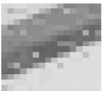
Figure 3.5: Visual artifacts of de-interplacing by merely performing spatial In-terpolation along the isophote direction.
In the Figure 3.5, we can see a lot of “salt and pepper”noises around the edge and those relative to pixel sites. These noises are caused by erroneous isophote lines determined roughly by slope identi…cation. Because of Prewitt operation only take the nearest six original pixels around interpolated pixel to calculate ISV. But the optimal match of slope of isophote found in the neighbor structure could be out of the range of Prewitt mask like direction labeled 0, 1, 9 and 10 in Figure 3.4. As discussed so far, isophote to be considered as local-smoothing information but weakly outside of nearest six neighbors.
In order to …x this problem, take the slope-determined direction at …rst step as prediction of smooth direction which is approximate to the real one. Next, we use the common method which is employed usually in EDI method that is minimizing the di¤erence between two intensities on the side of de…ned isophote. When searching every de…ned isophote in the neighboring structure, we apply a smoothness constraint factor to …nd the correct isophote. Eq. (3.4) expressed as follows:
arg min
k [ Ik+ jk lj] (3.4)
,where k and l are isophote index and slope-determined index in the neighboring structure respectively, and the smoothness constraint factor iso is set to 5
empir-Figure 3.6: Subjective quality of the de-interplaced images using the smoothness constraint.
ically. The smoothness constraint means that the tolerance of distance between k and l where k moves away from l. The value of Ik have to get smaller if k is
correct one. The Figure 3.6 shows the ideal spatial interpolation after correction.
3.1.2
Adaptive Decision of Dominant Edge
The objective of proposed statistic method is looking for the “dominant edge” adaptively. First, the statistic method de…nes a sample scope which is size of 8x8 block involve original and missing pixels. There are 32 interpolated pixels involved. Next, take the interpolated pixel as center of neighboring structure illustrated in Figure 3.4 to calculate intensity variation for every de…ned isophote for each interpolated pixel in the sample scope. All the intensity variations for every de…ned isophote direction in neighboring structure are calculated. Let fj Ikjg denotes the
set of magnitude value of intensity variation with index k and fj Ik10%jg denote the
set of the top 10% values in the data set fj Ikjg. Assume that top 10% intensity
variation fj Ik10%jg represents discontinuity features of isophote direction k in
the sample scope. Let j Ik90%j represent the minimal value in fj Ik10%jg. Let
fj IDFjg denote the collection of j Ik90%j for all isophotes in the structure. The
The sample block involves apparent edge if j IDFj is small. On the other
hand, it represents there is non-distinguishable edge if j IDFj is large. We use
this feature to …nd out the dominant edge by the following discriminant: if IS> j IDFj
The pixel at dominant edge;
where IS represents the strength of isophote which is set equal to jiso_vj + jiso_hj. If IS is small than j IDFj that it represent the site of pixel at dominant
edge. But this detection is not robust in the texture image. Because of the j IDFj
could be so large that it cannot …nd out the dominant edge even it is exists. After dominant edge detection, the pixel value of spatial interpolation using linear average two pixels along the isophote direction which founded in section 3.1.1.
3.2
Proposed Motion Compensated Interpolation
This section considers the temporal method for interpolating missing line. The results of temporal interpolation usually have better visual quality than results of spatial interpolation given correct motion information like stationary pixel and motion vector. In our temporal method, the interpolation comes from neighboring …elds, backward …eld and forward …eld. We take two methods for interpolating missing line, motion adaptive and motion compensation.
3.2.1
Vertical Even-step of MV Search Window
In four-…eld motion compensation, the method takes four …elds as reference …eld for motion estimation to obtain motion vector and then compensate the missing line of current processing …eld [3][4]. We use the concepts of four-…eld motion estimation and modify it to obtain reliable motion vector for compensation.
t t-1 x x t-2 0 -1 -2 1 2 3 4 x x o o o x x x x x x o o v e rt ic a l p o si ti o n evenverti cal motion (a) t t-1 x t-2 0 -1 -2 1 2 3 4 x o x x x x x x o o o odd vertical m otion v e rt ic a l p o si ti o n (b)
Figure 3.7: Comparison of (a) odd-valued and (b) even-valued vertical displace-ments.
As shown in Figure 2.12, the method of four-…eld motion estimation [3][4] to estimate motion vector from the reference …eld. Suppose the current …eld corre-sponds to time t, we denote the …eld at time t 1 as backward …eld, back-backward …eld at time t 2, and denote the …eld at time t + 1 as forward …eld. The motion estimation is performed between back-backward and forward …elds. After mo-tion estimamo-tion, all of the compensated pixel values come from the …elds at time t 1 and t + 1. In [6][20], the authors mentioned that a velocity leading to an odd-vertical integer pixel displacement between two successive …elds would cause a problem of true data lost in the temporal order. The problem is called “critical velocity” illustrated by the Figure 3.7(b).
As shown in the Figure 3.7(b), the image data which is considered to be trans-mitted toward the current …eld over trajectory would disappear at time t 1. If an object moves vertically in odd number lines between two sequential …elds, the existing lines of the object in the current …eld do not change in all reference …elds. According to the reason mentioned above, the odd-vertical motion makes the im-age data disappear. To prevent that erroneous MV we modify the search window into vertical even-step, the range of which should range from f: : : ; 2; 0; 2 : : :g. For discarding the dangerous MVs, it reduces not only erroneous MVs but also computing complexity due to only half of MV search window has to be considered.
3.2.2
Match Criterion with Smoothness Constraint
The purpose of common motion estimation in video coding is to minimize the energy of residual images as much as possible. But the motion estimation in de-interlacing algorithm aims at not only minimizing the energy of residual in same parity …elds but also the MV di¤erence to its neighborhoods, which is the property of "True" motion. There are two conditions have to be considered about the MV di¤erence, temporal and spatial continuity of motion vector. It means that motion vector of current block should have similarity to at least one of its neighboring block. Therefore, we add a smoothness constraint into matching criteria for motion estimation.
Usually, one of the popular matching criteria to minimize the energy of resid-ual is sum of absolute di¤erence (SAD). In addition to SAD, motion di¤erence between its neighbors including temporal and spatial block were calculated. By introducing the continuity and smoothness constraint, the equation of proposed matching criterion 3.5 and neighboring blocks is shown in Figure 3.8:
In the Figure 3.8, the motion vector with double indices, M V (x; y), which is estimated motion vector of current block. The motion vector with one index,
MV0 MV(x,y)
MV2 MV3
MV4
MV1
t-1
t
Figure 3.8: Estimated motion vector M V (x; y) and its …ve neighbors located at spatial and temporal respectively.
M V n, represents the neighboring motion vector around current motion vector. M V (x; y) = arg min j [SAD1j + SAD2j + mvDj] (3.5) Dj = X 0 n 4 jjMVj M Vnjj (3.6)
In Eq. mv is smoothness constraint of motion vector, Dj is sum of the
di¤er-ence of current motion vector with index j in search window and its neighboring motion vectors. We employ the SAD matching criterion referenced in [3], and mv
to formulate the proposed matching criterion. The value of mv represents the
importance of motion continuity. If mv is larger, D will be more signi…cant in
proposed matching criterion. But the value of mv should not be too high because
a high value of mv would make the SAD lose its signi…cance in matching
crite-rion. Hence, the dominant motion vector is determined by D only. However, the smoothness constraint would also a¤ect the performance of motion vector protec-tion strategy, which will be discussed later.
3.3
Proposed MV Protection Strategy
In chapter 2, we have discussed the motion compensation method already. It has the best quality of interpolation; however we did know that motion compensation also produces serious annoying block artifacts. Most of block artifacts are caused by erroneous MV which is the MV will cause a serious block artifact, and it’s very hard to …nd out the erroneous MV. In this section, we introduce two types of discontinuity measurement: local and contextual discontinuity [5] in the calculation of motion vector energy (MVE) to detect which MV is reliable and which MV is unreliable.
3.3.1
Motion Vector Reliability (MVR) Problem
There are two types of MVR problem, missing detection and false detection, when detecting whether MV is reliable or not. The …rst problem is that the erroneous MV can not be found by the MVR detection. The second one is that the good MV is detected as erroneous MV. This situation may cause serious annoying artifact, since the erroneous MV which causes the error result may be detected as a reliable one. While the MV which results good temporal interpolation may be detected as an unreliable one. This problem is more complex than the …rst one, since if the problem happens at position where spatial method do well, but blurring image at position unsuitable for spatial method.
3.3.2
MV Local Discontinuity
In [5], the author suggested a spatial gradient to an approximately estimated in a nearest neighborhood of certain pixel in image. Here, we introduce this concept of local discontinuity but not calculation of spatial gradient. Under the conditions of true motion, spatial continuity, we can assume that if the current MV is true
motion, then there must be at least another similar true motion MV in one of neighboring blocks. First, we de…ne the nearest neighborhood around the current block.
N (x; y) =f(i; j)jjx ij 1;jy jj 1g (3.7) By the condition, we modify the calculation of local discontinuity like following equation:
h(x; y) = min
N (x;y)fkMV (x; y) M V (x + i; y + j)kg (3.8)
where h(x; y) is a measurement of local discontinuity. We calculate the two-norm of MV di¤erence between its entire neighborhoods, then h(x; y) is set equal to the minimal di¤erence between current motion vector and its neighboring motion vectors. If h(x; y) is large than a small threshold value T Hld like 0 or 1, we can
consider the current motion vector is not a true motion. Because the assumption of spatial continuity is failed and no true motion block is around. If current motion vector is not a true motion, it is considered as an unreliable motion vector.
3.3.3
MV Contextual Discontinuity
After the MVR determination of local discontinuity, there are lots of block artifacts preserved. We call those MVs as “missing detection,” due to missing recognition of erroneous MV, see following Figure 3.9.
The local discontinuity is not robust enough because the noise is substantial in a fast movement. The measurement cannot distinguish true motion from the cluster of erroneous motion vectors. In order to enhance the measurement of MV discontinuity, should be extended a MV di¤erence to the summation of MV di¤erences of its neighborhoods, which is called contextual discontinuity [5]. In [5], the pixel-based contextual information could be thought as the correlations of pixel and its neighboring pixels as well as the theorem of markov random …eld [16]. We
(a) (b)
Figure 3.9: (a) MC only picture, (b) After true motion detection.
translate pixel-based contextual information to MV-based contextual information for calculating the MV discontinuity, which is translated into motion vector energy (MVE). The value of MVE means that the energy between the current motion vector with its neighborhoods; therefore we recognize that the motion vector is reliable if the MVE is small enough. The structure, which contains 8 neighboring MVs, N (x; y) is same as the evaluation of local discontinuity.
H(x; y) = P
i;j2N(x;y) k MV (x; y) M V (x + i; y + j)k
jN(x; y)j (3.9) In Eq. 3.9, H(x; y) is measurement score of contextual discontinuity. In the MVE detection, if the value of H(x; y) small than a prede…ned threshold T Hcd ,
the current motion vector would be recognized as unreliable motion vector, vice versa. Then, the contextual discontinuity detection follows the local discontinuity detection, the result of interpolation is shown as following:
As shown in Figure 3.10, the most of erroneous motion vectors were detected correctly. After identifying the erroneous motion vectors, the problems of MVR, “missing error” and “false detection,” are presented. The following section will disscuss the MVR problem whether the motion vector is estimated with the
smooth-Figure 3.10: Result of true motion and MVE detection.
ness constraint or not.
3.3.4
Irregular and Regular MVs
In this section, considering two distributions of MVE which are produced by the matching criterion with smoothness constraint and without smoothness constraint respectively. The …rst thing to be considered is the motion compensated picture which depends on motion vectors, which are produced from SAD matching criterion without smoothness constraint. For example, the Figure 3.11.
As shown in Figure 3.11 (a), the motion compensated picture at 190th frame in foreman sequence. That is fast motion with scene change. The MVE distribu-tion graph is shown in Figure 3.11 (b) which maps to Figure 3.11 (a). There are high-value, messy MVEs distributed at not only moving object (electric tower and foreman’s arm) but also smooth area (sky) in whole picture. This kind of distribu-tion may imply a lot of “false detecdistribu-tions.”As mendistribu-tioned in secdistribu-tion 3.3.1, the false detection may not cause serious artifacts. But if the position of false detection is not suitable for spatial method, it will cause blurring image and ‡ickering in display.
(a) (b)
Figure 3.11: (a) MC picture at 190th frame in foreman sequence, (b)MVE dis-tribution relative to (a).
(a) (b)
( 0, 1) ( 0, 1) ( 0, 1) ( 0, -2) ( 0, 9) ( 0, 1) ( 0, -13) ( 0, -16) ( 0, 15)
(c)
Figure 3.12: (a) Good MC picture in coastguard sequence. (b) False detection caused by irregular MVs surrounding. (c) Neighboring MVs of current MV in (b).
In Figure 3.12 (a), which represents a good motion compensated image; how-ever, the corresponding motion vector is detected as unreliable motion vector and it blurs the image as shown in Figure 3.12 (b). Because of the motion vector …eld (0,-9) (center of red grid in Figure 3.12 (c)) is signi…cantly di¤erent from its neigh-borhoods. Hence, the MVE of this motion vector is high and it would be turned to spatial interpolation. In fact, the position is not suitable for spatial interpolation due to horizontal edge being present.
In order to reduce the number of false detection, we modify the typical matching criterion without smoothness constraint into matching criterion with smoothness constraint such that regular motion vectors surround current motion vector. By modifying the matching criterion, the MVE distribution Figure 3.11 (b) is changed. Comparing the Figure 3.11 (b) with Figure 3.3.4, the Figure 3.3.4 forms the shape of moving objects and the value of every MVE in smooth area becomes small. Using the result, the MV in smooth area would always be considered as reliable MV, since those MVs become smooth and toward same direction. Using the behavior, we can apply a small threshold to detect the moving object because
the moving object always makes the MV erroneous. Therefore, if the MVEs across entire image is reduced such that the number of false detection will decrease; especially in the image feature that spatial method is useless like horizontal edge.
3.3.5
Autocorrelation Detection
The frequency of false detection is decreasing due to proposed matching criterion, especially the blocks in smooth area. On the other hand, the number of missing detections in entire sequence is increasing. It is imaginable that the additional instances of missing detection happen in the smooth block with fast motion because proposed matching criterion make the smooth block get low MVE. In order to …x this problem, we introduce a column-wise autocorrelation inside the block with reliable motion vector to re…ne such problem, which is calculated by :
Rk(l) =
E[(I(x; y) )(I(x; y + l) )]
2 (3.10)
where Rk(l)is autocovariance at column k and shift l step in vertical direction, and
and 2are mean and variance of pixels in column k respectively. The detection of
method is to calculate the value of autocovariance corresponding column number and shift one step vertically until bottom of intensity block. After calculating the autocovariance value each row in column, it forms a serious of autocovariance value. If the sequence of autocovariance value represents a periodic wave like Figure 3.13, this block is the case of missing detection.
If the periodic wave is shaking back and forth between positive and negative, the block is detected as unreliable MV. That is a special case for missing detection happened in the smooth area.
Figure 3.13: Periodic wave in sequence of autocovariance values. if Stationary pixel site ? if MV Reliable ? MC
Interpolation InterpolationSpatial
It(x,y)
Output
1( , ) 1( , ) 2 t t I− x y +I+ x y Highest priority2nd priority lowest priority
3.3.6
Stationary Pixel Detection and Output Decision
The site of interpolated pixel has to be considered as stationary or non-stationary in proposed de-interlacing algorithm. The proposed method refers to three-…eld motion detection which has been discussed in prior section, and take the MV information to decide the site of interpolated pixel is static or not. If the current pixel position is within a certain block in which the motion of the block is zero motion, the current pixel position would be considered as stationary. As shown in Figure 3.14, it is clear that temporal interpolations have higher priority than spatial interpolation.
CHAPTER 4
Experimental Results and Analysis
The peak SNR (PSNR) is used as the objective measure criterion to measure the quality of the de-interlaced frames in the simulations of proposed de-interlacing algorithm.
4.1
Analysis of MV Smoothness Constraint
In proposed de-interlacing algorithm, the smoothness constraint for motion vector mv has to be considered. In order to analyze the in‡uence of mv, the
performance of motion compensation and de-interlaced result are taken account for test sequences with varying mv. The con…gurations of mv are discrete integer
values in this analysis, which are {0, 1, 5, 10, 11, 12, 13, 14, 15, 16, 17, 50, 60, 75, 100}, and the testing parameters are shown in table 4.1.
Table 4.1: The testing parameters.
Local discontinuity threshold Contextual discontinuity threshold T Hld T Hcd
0 3
The value of mv would in‡uence the performance of proposed MC
de-interlacing algorithm directly because the reference …elds of MV search win-dow (same parity …elds) and motion compensation (opposite parity …elds) are di¤erent. As shown in the Figure 4.1, the both performances of MC re-sult and de-interlaced rere-sult are growing with increasing mv under the …xed
con…guration of MV protection strategy. The Figure 4.1(a) and (b) show the gap between two results where represents the performance of de-interlaced result is better than MC result due to block artifacts were detected.
The average PSNR values of most test sequences are monotonically increas-ing with mv increasing in a certain range. However, if the value of mv
changes and moves away out of the range, the average PSNR values will start to decrease, see the Figure 4.1(a) and (b). The behaviors of most motion vectors in an image are following its neighboring motion vectors regardless of block residual energies when mv is large. The block residual energies are
im-neglectable because it would in‡uence the visual quality of de-interlacing directly, like occlusion area and fast motion Figure 4.2.
The analysis of test sequences like "Container" and "Coastguard" (Figure 4.1), in which the PSNR curves are closed. It is because the moving objects in both sequences which are slow and stable motions in whole sequence. In such sequences, the motion compensation performs well even more e¢ cient than de-interlaced result.
(a) (b)
(c) (d)
Figure 4.1: The in‡uence of Landa MV for sequences. (a) Foreman. (b) Stefan. (c) Coastguard. (d) Container.
(a) (b)
Figure 4.2: Artifact caused by large landa (a) Occlusion area, the foreman’s tongue. (b) Fast motion.
In the observation, the upper boundary of that range is 10. Hence, setting the value of mv equal to 10 is reasonable in the proposed algorithm.
4.2
Analysis of Reliable and Unreliable Blocks
The numbers of unreliable and reliable blocks entire sequence are di¤erent between the MVs produced from ME with and without smoothness constraint. The behavior of MVs entire image would get messy if the MVs are produced from ME without smooth constraint. The messy MV distribution may imply many cases of false detection, especially the neighboring similar blocks. Those blocks with similar spatial feature clustered together may have di¤erent MVs; but under the assumption of continuity, those blocks should have similar MVs in fact. The Figure 4.3 shows the number of unreliable blocks between the MEs with and without smoothness constraint.
In the Figure 4.3, the blue bar presents the total number of unreliable blocks in the entire sequence without MV smoothness constraint, and red bar presents the
Figure 4.3: Total number of unreliable blocks entire sequence.
total number of unreliable blocks entire sequence with MV smoothness constraint. Particularly, those sequences of "Foreman", "Dancer" and "Stefan," have lot of smooth blocks in fast motion and therefore, there is great probability that those smooth blocks are detected as reliable. In fact, most of those blocks are not reliable because they missed the detection. In order to identify those blocks as unreliable, the autocorrelation detection is needed.
As shown in the Figure 4.4, the green bar which represents the number of unre-liable blocks is rising because the autocorrelation corrects the problem of missing detection.
4.3
Comparison of Subjective Quality and PSNR
To show the objective measurement of proposed de-interlacing algorithm, there are 10 test CIF sequences and 2 test QCIF sequences for calculation of aver-age PSNR value. Those sequences are standard test sequences of video coding,
Figure 4.4: Total number of unreliable blocks entire sequence with column-wise autocorrelation.
such CIF sequences are "Aikyo", "Bus", "Coastguard", "Container", "Dancer", "Foreman", "Stefan", "Table tennis", "Silent" and "Mobile", and the other two QCIF sequences are "Hall monitor" and "Mother and daughter." The Figure 4.5 illustrates the test environment of proposed de-interlacing algorithm. First, the frame sequence is down-sampled from progressive CIF 352x288 or QCIF 176x144 to interlaced sequence 352x144 and 176x72 at rate 30 …elds per second. Second, the test interlaced sequence produced from interlacer is input of our proposed de-interlacing algorithm. Finally, the output of de-de-interlacing algorithm is progressive sequence at 30 frames per second and is used to evaluate the PSNR comparison with original progressive sequence without down-sampling.
The subjective results of proposed isophote spatial interpolation, motion com-pensation and …nal output are shown from Figure 4.6 to Figure 4.10 respectively, and the table 4.2 shows the average PSNR value from six di¤erent methods and those are plotted in Figure 4.11. Apparently, the proposed de-interlacing algorithm
CIF or QCIF Interlacer Proposed Deinterlacer Compare PSNR 30 fields/sec 30 frames/sec 30 frames/sec 30 frames/sec
Figure 4.5: Test ‡ow.
obtains the better PSNR than other de-interlacing algorithm.
Although the proposed algorithm has e¢ cient objective quality, the "Missing detection" and "False detection" problem still exist in de-interlaced sequences. The proposed MV protection strategy is not robust enough because there are too much noises of MV di¤erence to distinguish the motion vector are useful or useless. To show the bene…ts and drawbacks of proposed de-interlacing algorithm in subjective quality, we do the comparison with reference software STCAD from Media SoC Lab of National Cheng Kung University (sincerely thank Prof. Gwo-Giun Lee). The left column of pictures in Figure 4.12(a) and 4.13, the shaking edge appeared in the result from STCAD; on the other column, the edge at same place getting more smooth in proposed algorithm. It can show that the proposed algorithm performs well than STCAD.
Because the problems of "Missing detection" and "False detection" are not cleared completely, so the block artifacts would appear sporadically, in which are shown in Figure 4.14 and 4.15.
(a)
(b)
(c)
Figure 4.6: The experimental result for sequence "Foreman", "Bus." (a) Isophote interpolation. (b) Motion Compensation. (c) Hybrid.
(a)
(b)
(c)
Figure 4.7: The experiment result for sequence "Aikyo", "Coastgurad."(a) Isophote interpolation. (b) Motion Compensation. (c) Hybrid.
(a)
(b)
(c)
Figure 4.8: The experiment result for sequence "Mobile", "Container."(a) Isophote interpolation. (b) Motion Compensation. (c) Hybrid.
(a)
(b)
(c)
Figure 4.9: The experiment result for sequence "Table", "Stefan." (a) Isophote interpolation. (b) Motion Compensation. (c) Hybrid.
(a)
(b)
(c)
Figure 4.10: The experiment result for sequence "Silent", "Dancer." (a) Isophote interpolation. (b) Motion Compensation. (c) Hybrid.
Table 4.2: Table of PSNR Comparison.
Sequence HVMD TDMD AMD WRELA STCAD 4-…eld Proposed [18] [22] [25] [12] GMC/MC [3] Algorithm Aikyo 45.64 41.4 45.29 45.68 48.45 N/A 48.16 Dancer N/A N/A N/A N/A 37.69 N/A 38.00 Bus N/A N/A N/A N/A 29.18 N/A 29.26 Container 40.19 29.98 35.41 34.85 41.52 40.17 45.07 Coastguard 33.16 28.30 31.06 31.04 32.60 33.30 36
Foreman 30.18 33.56 33.20 35.11 35.10 34.37 36.22 Stefan 23.79 24.83 27.86 27.73 28.22 26.12 29.61 Silent 36.55 35.91 41.80 41.52 42.48 40.37 42.65 Table tennis N/A N/A N/A N/A 36.43 35.20 37.26 Mobile 24.22 23.43 26.71 27.46 29.59 25.93 30.01 Hall monitor 40.94 33.05 38.55 39.96 41.24 40.04 43.35 M&D 43.79 40.12 42.67 45.96 46.30 44.83 47.71 Average 35.38 32.29 35.83 36.59 37.40 35.09 38.61
(a) (b)
Figure 4.12: The comparison of experimental result for sequence "Foreman", "Bus" and "Table." (a) STCAD results in left column. (b) Proposed de-interlacer results in right column.
(a) (b)
Figure 4.13: The comparison of experimental result for sequence "Dancer", "Coastguard" and "Container." (a) STCAD results in left column. (b) Proposed de-interlacer results in right column.
(a) (b)
Figure 4.14: The missing detections in proposed algorithm. (a) Block artifacts of proposed algorithm in left column. (b) Better results of STCAD in right column.
(a) (b)
Figure 4.15: The fasle detections in proposed algorithm. (a) Blurred image of proposed algorithm in left column. (b) Better results of STCAD in right column.
CHAPTER 5
Summary and Conclusion
5.1
Summary
In this thesis, we propose several methods for de-interlacing algorithm. These methods can produce satisfactory output of de-interlacing not only for human vision but also objective measurement.
The proposed methods are follows: 1. Spatial Interpolation
Approximate smooth edge: To estimate an approximate smooth edge according to the isophote direction.
Smoothness factor correction: Correcting the approximate smooth edge. Statistic dominant edge: Creating an adaptive dominant edge detection.
2. Temporal Interpolation
Vertical even-step search window: Reducing the vertical odd-step mo-tion for avoiding absence of image in interlaced scan.
Smoothness constraint matching criterion: To produce the regular mo-tion vectors in similar region.
3. MV Protection strategy
Local and contextual MV discontinuity: For calculating the energy of motion vector to recognise erroneous motion vector.
Autocorrelation detection: This detection is a MV post-protection es-pecially for feather e¤ect in smooth block with fast motion.
5.2
Conclusion
The most problems of proposed isophote interpolation we have met, which are often happen on certain special image feature, like near-horizontal edge. The near-horizontal edges have not been de-interlaced as well as other directions in the de…ned neighboring structure. That is because the near-horizontal edges exceed the direction resolution of de…ned neighboring structure. The larger neighboring structure and gradient operator would solve such problem due to higher direction resolution.
In MV protection strategy, we disregard using the analysis of spatial feature against signi…cant block artifacts caused by erroneous MV. By de…ning the energy calculation under the property of continuity of "True motion" assumptive, a min-imal MV energy state is related with MV behaviors that have similarity between the neighboring MVs. Applying proposed algorithm to MV protection strategy, most of erroneous MVs in the test sequences were detected. In addition to MV protection strategy, we also make the behavior of MVs smooth to neighboring MVs
by MV smoothness constraint. This modi…cation makes the performance better on not only motion compensation but also MV protection strategy. In comparison with analysis of spatial feature MV protection algorithms, the proposed one is simple and useful at judgment of erroneous MVs.
At …nal output of proposed algorithm, we did use the great quantity of tem-poral interpolation as major interpolations, including the objective in motion or stationary. And the spatial interpolation can make up for the serious artifacts of temporal interpolation; therefore, the isophote and motion compensated interpo-lation are complementary. The proposed de-interlacing algorithm has eliminated the several problems in spatial interpolation successfully, like ‡ickering and blurred image, and serious artifacts of temporal interpolation is compensated by spatial interpolation.
5.3
Future Work
The missing detection of MVR problem would happen when object is moving in fast motion, and false detection would blur image which is unsuitable for spatial interpolation. Since a lot of noises of erroneous motion vector, the calculation of MVE cannot represent the erroneous motion vector. Therefore, the pixel-wise determination is expectable to solve such problem. It is clear that the spatial feature can still be taken into consideration in our future analysis. In order to determine the output, it is critical to avoid the weakness of spatial feature and combine the advantages of spatial feature and temporal information in our future analysis.
Bibliography
[1] C. Ballester, M. Bertalmio, V. Caselles, L. Garrido, A. Marques, and F. Ranchin, “An Inpainting-based Deinterlacing Method,” IEEE Transac-tions on Image Processing, vol. 16, pp. 2476 –2491, October 2007.
[2] M. Bertalmio, G.Sapiro, V. Caselles, and C. Ballester, “Image Inpainting,” Proceedings of the ACM SIGGRAPH Conference on Computer Graphics, pp. 417 –424, 2000.
[3] Y. L. Chang, S. F. Lin, C. Y. Chen, and L. G. Chen, “Video De-interlacing by Adaptive 4-…eld Global/Local Motion Compensated Approach,”IEEE Trans-actions on Circuits and Systems for Video Technology, vol. 15, no. 12, pp. 1569 –1582, December 2005.