行政院國家科學委員會專題研究計畫成果報告
計畫名稱:自行車傳動系統測試軟體之類神經網路結構最佳化設計
計畫編號:NSC90-2212-E009-039 執行期限:90 年 8 月 1 日至 91 年 7 月 31 日 主 持 人:曾錦煥 交通大學機械系 教授 摘要 利用最佳化方法設計類神經網路的結 構參數,可以提升類神經網路的效能。本 研究計畫利用最佳化方法中的田口方法與 實驗設計法,進行類神經網路中結構參數 的最佳化設計。在最佳化過程之前,使用 者須先選擇一個適合的類神經網路模型, 而後再依據此類神經網路模型定義最佳化 問題的形式。在最佳化過程中,本研究計 畫將先利用田口方法找出較重要的結構參 數,然後再利用實驗設計法分析這些重要 的結構參數對類神經網路效能的影響。最 後,經過最佳化設計的類神經網路模型應 用在自行車傳動系統的測試系統上。 ABSTRACTThe integration of neural networks and optimization provides a tool for designing the network parameters and improving the network performance. In this study, the Taguchi method and Design of Experiment (DOE) methodology are used to optimize the network parameters. The users have to recognize the application problems and choose a suitable Artificial Neural Network (ANN) model. Then, the optimization problems can be defined according to the model. The Taguchi method is first applied to the problem for finding the more important factors. Then DOE methodology is performed for further analysis and forecast. An LVQ example is demonstrated for the application to bicycle derailleur systems.
Keywords: Neural networks; optimization; Taguchi method; design of experiments; bicycle derailleur systems.
INTRODUCTION
Artificial Neural Networks (ANNs) are
receiving much attention currently because of their wide applicability in research, medicine, business, and engineering. ANNs offer improved performance in areas such as pattern recognition, signal processing, control, forecasting, etc.
In this study, a systematic process is introduced to obtain an optimum design of a neural network. The Taguchi method and the Design of Experiments technique (DOE) (Montgomery, 1991) are the main techniques used. Unlike previous studies, the Taguchi method is used here to simplify the optimization problems. Then, DOE is more easily performed. Because of the stronger statistical basis of DOE methodologies, many analyses can be executed. Finally, a Learning Vector Quantization (LVQ) network is demonstrated as an example. The method proposed in this paper can also be applied to any ANN model. The integration of optimization and ANNs in this paper was simulated by a computer program which can be executed automatically and easily.
THE EXAMPLE
In order to demonstrate the optimum design processes, an application with a Learning Vector Quantization (LVQ) model is shown. In this example, the purpose is to distinguish the type of chain engagement to be used in the rear derailleur system of a bicycle.
1. Pr oblem descr iption
The derailleur system in a bicycle is similar to the gear box in a motor vehicle. A complete derailleur system, as shown in In derailleur system designs, two types of chain engagement, Type I and Type II, have to be considered (Wang et al., 1996). The
the two types are different; therefore, it is very important for the designers to know which type occurs during each gear shift. So, the different design defects for the two types can be found and improved.
In a real riding or testing environment, it is very difficult to distinguish which type of chain engagement occurs. There must be a camera for monitoring purposes. This costs a lot of money and it is not very easy to install. The purpose of this example is to establish a better and easier method to distinguish the chain engagement type during gear shifts, using a neural- network model.
The data fed to the network are transferred from the time domain to the frequency domain by the FFT technique (John and Dimitris, 1996). In gathering training data, if the tooth numbers of two adjacent sprockets are both even and the tooth number of the chainwheel sprocket is also even, only one type of chain engagement will occur. If only one chain link is shifted from the previous situation, another type will occur.
2. Choosing an ANN model
In supervised learning models, an LVQ example like that shown in Fig. 7 is selected because of this fast training speed, no local minimum traps and better performance in classification (Patterson, 1996). The LVQ is the transformation from the input vector x
of dimension n to known target output
classifications t(x)= t, where each class is
represented by a codeword or prototype vector w (i=1, 2, ..., m). The index i is i
the class label for x. Let C(x) denote the
class of x computed by the network; w is c the weight vector of the winning unit c.
Then, C(x) is found using
wc−x =mini wi −x .
When the class is correct, i.e. C(x)= t,
the weight vector of the winning unit c is
shifted toward the input vector. When an incorrect classification is selected, i.e. C(x)≠t, the weight vector is shifted away from the
input vector. The update rule for the LVQ can be summarized as follows:
1) Initialize the weights w to small
random numbers.
2) Find the prototype unit to represent x
by computing
wc −x =mini wi −x .
Update the weight vectors according to c i w w t x C w x w w t x C w x w w old i new i c old c new c c old c new c ≠ = ≠ − − = = − + = − + all for ) ( if ) ( ) ( if ) ( α α where 0 0 > > − + α α
are the learning coefficients of two different cases. 3) Repeat steps 2 and 3 until the weights
stabilize.
3. Define the optimization pr oblem
The optimal physical problem can be covered by a mathematical model of design optimization involving the procedures below.
1) Choose design variables. In this example, the chosen design variables from the LVQ network parameters are the number of input units, α and + α , and the weight − initialization range. The number of input units is a discrete design parameter, α+ and α− are continuous design parameters, and the weight initialization range is a qualitative design parameter.
2) Define an objective function: The objective function in this example is defined as the grouping error of the network, cost function = ( ( ), i) i i diff C x t f
∑
, where ≠ = = = i i diff i i diff t x C f t x C f ) ( if 1 ) ( if 0data. The output of interest of this example is a “smaller-the-better” quality characteristic.
3) Identify constraints. A suggested range of design variables from the solver SNNS (Zell, 1995) will be described in next section.
4. The Taguchi Method
The theories and principles used in the Taguchi Method (Taguchi, 1986; Peace, 1993) will not be described in detail; only the key points and analyzed results are shown below.
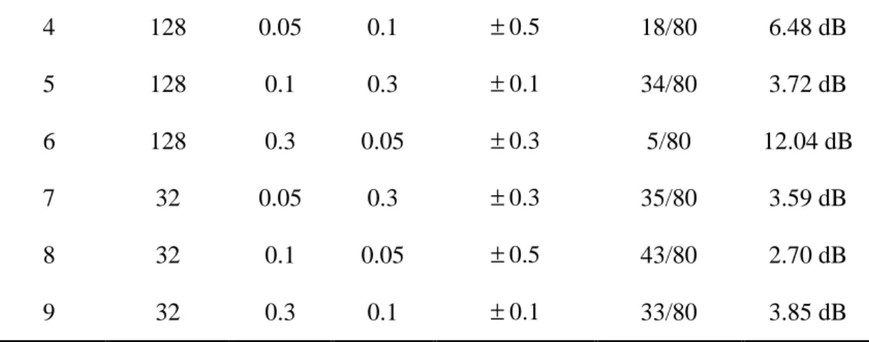
1) For the number of input units; the vibration signals during gear-shifting are transformed into the frequency domain by the FFT to 256 data points. Therefore, in this factor (the number of input units), three levels (256, 128 and 32 points) are selected.
2) 0.05≤α+,α− ≤0.3 is assumed, and three levels (0.05, 0.1 and 0.3) are selected.
3) For the weight initialization range, a small range is suggested from the software (Zell, 1995). Therefore,
5 . 0 and 3 . 0 , 1 . 0 ± ± ± are selected.
After the factors and levels are determined, a suitable orthogonal array can be selected for the training process. Table is the L9(34) orthogonal array for the factors and levels in this example. For instance, in the first training experiment, there are 256 input units, η and + η are − set to 0.05, and the weight initialization range is between +0.1 and -0.1. After nine training experiments have been made, the grouping errors of the 80 training data are summarized in Table 1. Because there are no local minimum traps in this model, replicate training is not needed for the same parameters. For some other models, the final results may be affected by different initial designs. Therefore, replicated training is necessary for the following S/N
analysis.
The last column in Table 1 is the signal-to-noise ratio (S/N). The equation for calculating the S/N for the smaller-the-better quality characteristic is Equation A.1. In this example, there is only one replicate, therefore, the physical meaning of S/N is similar to the grouping errors in Table 1. The grouping errors are used here instead of S/N for easier understanding.
The next step in the Taguchi method is Level Average Analysis. The goal is to identify the strongest effects, and to determine the combination of factors and levels that can produce the most desired results. Table 2 is the response table, which shows the average experiment at result for each factor level. The total effect of the 256 input units is 16. This is the average grouping error of the first three rows in Table 2 ((1+14+80)/3=16). Other response values can be calculated by using a similar method. For the number of input units, 256 units can get a smaller grouping error than other levels. The same principle can be used to make η+ and η equal to 0.05, and the weight − initialization range to be between +0.3 and -0.3. Therefore, the recommended factor levels are: 256 input units, η+ =0.05 ,
05 . 0
=
−
η and a weight initialization range of ±0.3.
CONCLUSIONS
Optimization techniques have been widely used in many applications. In this paper, two major categories, the Taguchi method and the DOE methodology, are applied to improve one the original designs of ANNs. The users have to recognize the design problem and choose a suitable ANN model. Then, the optimization problems can be defined according to the model. The Taguchi method is first applied to find the more important factors, and to simplify the design problems. DOE methodologies are then used to find the sensitivity and a more precise combination of design parameters. The final results of the examples introduced
in this study indeed improve the initial designs and get a better performance.
Although only one ANN model, LVQ, is demonstrated in this paper, other models, such as ADALINE, MADALINE, Hopfield Networks, MLFF, Boltzmann Machines, Recurrent Neural Networks, Neocognitrons, etc., are also suitable. Many benefits can be mentioned. First, this is a systematic method to use for a neural-network design. It means that the engineer, whether or not he or she is experienced in ANN, the Taguchi method and DOE, can follow this process easily. Many commercial software packages can be applied, such as SNNS in ANN and SAS in the DOE. Second, it will not take too much computational effort and time. The results of the demonstrated examples can be obtained within 5 minutes with a Pentium-150 PC. This detail was not emphasized in this paper because it is not the major concern here. Finally, in engineering applications, it is not necessary to get a global optimization of the problems, because that takes too much time or the algorithms may be very complicated. The improvement of the original designs in an acceptable region is helpful for engineers.
REFERENCES
Arora, J. S. (1989). Introduction to Optimum Design. McGRAW-HILL Book Company. Gill, P. E., Murray, W., and Margaret, H. W.
(1981). Practical Optimization. Academic Press.
John, G. P. and Dimitris, G. M. (1996). Digital Signal Processing. Prentice-Hall, Inc.
Khaw, B. S. L., John, F. C., and Lennie, E. N. L. (1995). Optimum design of neural networks using the Taguchi method. Neurocomputing, 7, pp. 225-245.
Lin, T.Y., and Tseng, C.H. (1998). Using fuzzy logic and neural network in bicycle derailleur system tests”, Proceeding of the International Conference on Advances in Vehicle Control and Safety (AVCS’98), Amiens, France, pp. 338-343.
Miller, G. F., Todd, P. M. and Hedge, S. U. (1989). Designing neural networks using genetic algorithms. Proc. 3rd Int. Conf. On Genetic Algorithms, pp. 379-384.
Montgomery, D. C., 1991. Design and Analysis of Experiments. John Wiley & Sons, Inc.
Patterson, D. W. (1996). Artificial Neural Networks, Theory and Applications, Prentice Hall.
Peace, G. S. (1993). Taguchi Methods, A Hands-On Approach. Addison-Wesley Publishing Company.
Taguchi, G. (1986). Introduction to Quality Engineering, Asian Productivity Organization, Tokyo.
Teo, M. Y. and Sim, S. K. (1995). Training the neocognitron network using design of experiments. Artificial Intelligence in Engineering, 9, pp. 85-94.
Wang, C. C., Tseng, C. H. and Fong, Z. H. (1996). A method for improving shifting performance. International Journal of Vehicle Design, 18(1), pp. 100-117.
Zell, A. (1995). SNNS, Stuttgart Neural Network Simulator User Manual, Version 4.1, University of Stuttgart, IPVR, Report No. 6/95.
Input Units η+ η− Weight Initial Range Grouping Error S/N 1 256 0.05 0.05 ±0.1 1/80 19.03 dB 2 256 0.1 0.1 ±0.3 14/80 7.56 dB 3 256 0.3 0.3 ±0.5 34/80 3.72 dB
4 128 0.05 0.1 ±0.5 18/80 6.48 dB 5 128 0.1 0.3 ±0.1 34/80 3.72 dB 6 128 0.3 0.05 ±0.3 5/80 12.04 dB 7 32 0.05 0.3 ±0.3 35/80 3.59 dB 8 32 0.1 0.05 ±0.5 43/80 2.70 dB 9 32 0.3 0.1 ±0.1 33/80 3.85 dB
Table 1 Training results.
Factor Level Error Factor Level Error
256 16 0.05 16 128 19 0.1 22 Input units 32 37 − η 0.3 34 0.05 18 ±0.1 23 0.1 30 ±0.3 18 + η 0.3 34 Weight initial range 5 . 0 ± 32
Table 2 Response table.
Source Sum Square Degree of
Freedom Mean Square F0 Pr > F + η 141.56 2 70.78 0.42 0.6827 − η 205.56 2 102.78 0.61 0.5868 Error 673.11 4 168.27 Total 1020.23 8