研究氫原子下的pump probe 過程

國立交通大學

物 理 研 究 所

碩 士 論 文

研究氫原子下的 pump probe 過程

Study of pump probe process in hydrogen atom

研 究 生：鄭玉書

指導教授：江進福 教授

研究氫原子下的 pump probe 過程

Study of pump probe process in hydrogen atom

研 究 生：鄭玉書 Student：Yu-Shu Cheng 指導教授：江進福 教授 Advisor：Tsin-Fu Jiang

國 立 交 通 大 學

物 理 研 究 所

碩 士 論 文

A Thesis

Submitted to institute of Physics College of Science

National Chiao Tung University in partial Fulfillment of the Requirements

for the Degree of Master

in Physics July 2010

Hsinchu, Taiwan, Republic of China

I 研究氫原子下的 pump probe 過程 研究生：鄭玉書 指導教授：江進福 國立交通大學物理研究所碩士班 摘要 本篇論文研究以時間延遲的雷射脈衝研究電子波包。通過紅外雷 射游離激發態，脈衝雷射產生激發態和的電子波包，且在延遲下產生 新的連續的電子波包。從這二個步驟，分析分析波包的干涉，反映角 度解析的光電子光譜。使用分析表示，來探索信息的可能性關於雷射 脈衝所引起的電子波包。

II

Study of pump probe process in hydrogen atom

Student : Yu-Shu Cheng Advisor : Tsin-Fu Jiang

Institute of Physics

National Chiao Tung University Abstract

This thesis studies theoretically the electron wave packet generated

by an attosecond pulse train (APT) which is then probed with a time- delayed laser pulse. The APT creates an excited state and a continuum electron wave packet. By ionizing the excited state with an IR, a delayed new continuum electron wave packet is created. The interference of the wave packets from the two paths, as reflected in angle-resolved

photoelectron spectra, is analyzed analytically. Using the analytical expressions, we examine the possibility of retrieving information on the electron wave packet generated by the APT.

III

誌 謝

首先我要先感謝我的指導教授江進福教授，在平常從老師的身上 看到老師對研究專注的態度和熱誠，在學習研究上給予我許多建議及 指導。另外特別感謝李漢傑博士，在我有疑問時肯耐心地花時間指導 我和幫助我。也感研究室的鄭世達學長、張繼允學長在這過程的陪伴， 還有研究室同學吳明軒，一起討論、分享和許多意見交換。 也感謝壘球隊的伙伴，除了體諒我無法一起練球外也仍然給予我 鼓勵，還有教會親朋好友為了我的課業研究關心和代禱，最後要感謝 我的家人與女朋友的信任、肯定及支持與輔助，真是無比的感謝。

IV Index 摘要………..………I Abstract……….II 誌謝………III Index………...IV Index of figure………..V Chapter 1. Introduction………….………...………..………1

Chapter 2. Two-path interference model………2

Chapter 3. Simpler models for the calculation of transition amplitudes……….8

Chapter 4. Numerov method……….………...10

Chapter 5. First order time-depended perturbation to continuum………14

Chapter 6. Results………..20

Chapter 7. Conclusions.……….24

References……..……….………..…….25

V

Index of Figure

Figure 2-1 Pump-probe process………2

Figure 2-2 Single attosecond pulse (SAP)………3

Figure 3-1 Two-- state population 3fs FWHM and 2.5 TW/cm2………….6

Figure 3-2 Two --state population 3fs FWHM and 2.5 TW/cm2…………7

Figure 4-1 Numerov method in 1ev l=0…………...12

Figure 4-2 Numerov method in 5ev l=0………..13

Figure 5-1 M_𝐩,i X amplitudes in 3fs FWHM and 75TW/cm2.………16

Figure 5-2 M_𝐩,i X probability density in 3fs FWHM and 75TW/cm2….…16 Figure 5-3 M_𝐩,2p(L) amplitudes in 3fs FWHM and 55TW/cm2………18

Figure 5-4 M_𝐩,2p(L) probability density in 3fs FWHM and 55TW/cm2 …...19

Figure 6-1 M𝐩i(τ) 𝟐 in time-delay τ =τL 2 + τx 2………..20 Figure 6-2 M𝐩i(τ) 𝟐 in time-delay τ = τL 2 + τx 2 + 1………21

Figure 6-3 Angular distribution of photoelectron……….22

Figure 6-4 Interferogram dependence of on time-delay………23

1

1. INTRODUCTION

Attosecond pulse trains (APT) in the extreme ultraviolet (XUV) region have been produced in the process of high-order harmonic generation (HHG) by exposing rare gas atoms to intense femtosecond infrared (IR) laser pulses. These APT’s can span a broad spectrum of harmonics, each with a relatively narrow bandwidth, and in the time domain, a serious of attosecond bursts of radiation. Thus APT is suitable for initiating a dynamical atomic or molecular system which evolves nontrivially in time, while retaining spectral sensitivity. To probe such a wave packet in the laboratory, the most accessible tools are IR pulses that were employed to generate the APT, or the second or third harmonics of the IR. Such experiments have the advantage that the time delay between the APT and the IR can be controlled with high precision– at the level of attoseconds. Attoseconds is also the time scale needed in order to probe the electron wave packet dynamics generated by the APT.

The technology for producing APT or single attosecond pulses (SAP) is still in its infancy. Thus today only a handful of laboratories are capable of performing APT+IR or SAP+IR experiments. Ideally, the goal of a pump-probe experiment is to unravel the dynamic system after the pump. Since the dynamic system evolves in time, the probe pulse has to be applied at different delay times. While it may be of interest to observe how the results of the probe change with time delay, a more interesting and challenging question is how to retrieve information on the dynamic system from such pump-probe measurements.

2

2. Two-path interference model

By exposing a hydrogen atom to such an APT, the 2p state will be populated prominently among the excited states. In the meantime, the H atom can be ionized to the continuum directly. Clearly the efficiency of populating the 1s2p state and the width of the photoelectrons depend on the pulse duration of the APT.

After the pulse is over, another laser will be applied to the target again. Using laser the 2p state can be ionized by two-photon absorption to interfere with the wave packet generated directly, then a single-photon absorption will reach the same energy region.

The electron spectra are expected to show interference due to the two paths taken for the electron to reach the same kinetic energy after the probe. Here develop pump-probe model below where the time-delay dependence is given analytically.

For clarity, we define t=0 to be at the center of the APT pulse. The time difference between the APT and the IR is defined as the time delay, τ. The various parameters of the APT and the IR are clearly defined in Fig. 2-1 , about pulse defined in Fig. 2-2

Fig.2-1. Pump-probe process

1s 2p con.

−

𝛕

𝐱

𝟐

𝟎

𝛕

_𝐱

𝟐

𝛕 −

𝛕

_𝐋

𝟐

𝛕 𝛕 +

𝛕

_𝐋

𝟐

3

Fig.2-2. Single attosecond pulse (SAP) Δ= Full-Width-Half-Maximum (FWHM) pulse duration τ = 2.57757Δ n n=4~6 here always use n=6

time range= τ 2, − τ 2 H t = H₀ + zE_X t + zE_L(t − τ)

Consider the time evolution operator for the whole pump-probe cycle, we can write the total evolution operator as

U_total =U(τ+τL 2 ,τ-τL 2 )U(τ-τL 2, τx 2)U( τx 2,- τx 2)

For convenience, we define the propagators U_x≡U(τx 2,- τx 2 ; Ex t ) τx = 2.57757Δ n U_L≡U(τ+τL 2 ,τ-τL 2 ; EL t − τ ) τL = 2.57757Δ n (2.1) Such that Utotal =ULe− τ− τL 2− τx 2 H0U_x (2.2)

Here H0 is the field-free Hamiltonian and e − τ−τL

2− τx

2 H0 is represented in

terms of bound and continuum eigenstates |n> and eigenenergies ϵn of

H0 : e− τ−τL2− τx 2 H0= |n >_n e− τ− τL 2− τx 2 ϵn < 𝑛| (2.3)

4

Substituting this into (2.2), we can write the probability amplitude as a function of the time-delay τ for transition from initial bound state |i> to an ionized state with photoelectron momentum p as

M_𝐩i(τ)= e−i τ−τL2− τx 2 ϵn n M𝐩n (L) M_ni(X) (2.4) where M_ni(X) and M_𝐩n(L) are probability amplitudes for transitions

induced by XUV and IR pulses, respectively, M_ni(X) = n U_X i

M_𝐩n(L) = 𝐩 U_L n (2.5) Note that |p> is not a plane wave but a scattering wave which is an eigenstate of H0 with incoming boundary conditions. From the

expression (2.4) we can interpret the ionization process under the pump-probe as a coherent sum of paths represented by the intermediate states n.

Note that M_ni(X) and M_𝐩n(L) are independent of the delay-time τ. Once they are obtained, then we can generate the pump-probe interferogram M_𝐩i(τ) 𝟐as a function of τ for a given momentum p by using (2.4).

For hydrogen atom in the ground state exposed to the APT introduced previously, the transition amplitude M_ni(X) for bound states other than n=2p is negligible. Thus M𝐩i(τ) can be approximately

written as

M𝐩i(τ)=e−i τ−

τL 2− τx 2 ϵ2p M 𝐩,2p (L) M_2p,i(X) + e−i τ−τL2− τx 2 ϵ𝐩′ 𝐩′ M𝐩𝐩′ (L) M_𝐩′i(X) (2.6) where the second term on right-hand side represents the contribution from the intermediate scattering states |p’>. Since energy and momentum of a free electron are not changed by a laser field, the IR introduces a Volkov phase only.

5 M_𝐩𝐩′(L) ≈ δ(𝐩 − 𝐩′)exp − i 2 (𝐩 + 𝐀(t)) 2 τ 2 −₂τ dt (2.7) where 𝐄𝐋 t = − d𝐀(t)

dt and A is the vector potential describing the IR

laser pulse.

Using this approximation, M𝐩i can be written as a coherent sum of

contributions from the two paths, M_𝐩i(τ)=e−i τ−τL2−

τx 2 ϵ2p M 𝐩,2p (L) M_2p,i(X) + e−i τ−τL2− τx 2 ϵ𝐩e−i(τLϵ𝐩+𝛂∙𝐩+β) _M 𝐩,i (X) (2.8) where 𝛂 = 𝐀 t dt τ 2 −τ 2 and β = A2 t dt τ 2 −τ 2 (2.9) Here the transition amplitudes M_𝐩,2p(L) , M_2p,i(X) , and M_𝐩,i(X)can be respectively obtained, for example, by solving the corresponding time-dependent Schröedinger equations. Introducing their magnitudes and phases such that

M_𝐩,i(X) = a_𝐩eiφ𝐩 _{, M} 2p,i (X) = a_2peiφ2p _{, and M} 𝐩,2p (L) = b_𝐩,2peiϕ𝐩,2p _, (2.10) the ionization probability density is expressed as

M_𝐩i(τ) 𝟐 = a_𝐩2 + a_2p2b_𝐩,2p2 + 2a_𝐩a_2pb_𝐩,2pcos Φ𝐩,2p − (ϵ𝐩− ϵ2p)τ (2.11) with Φ_𝐩,2p = φ_𝐩 − (ϵ𝐩τL + 𝛂 ∙ 𝐩 + β)-( φ2p + ϕ𝐩,2p)+( ϵ𝐩 − ϵ2p)( τL 2 + τx 2) (2.12) Note that the sinusoidal τ-dependence of M_𝐩i(τ) 𝟐 is explicitly shown in (2.11).

6

3. Simpler models for the calculation of transition amplitudes

In the previous subsection, the effect of the pump beam is obtained by solving the time-dependent Schrödinger equation (TDSE) with a model potential for hydrogen. Since the XUV pump is not exactly in the strong field regime, it is preferable that the scattering amplitudes from the pump pulse be solved using perturbation theory. However, the pump laser is nearly resonant with the 1s to 2p transition, the scattering amplitude M_2p,i(X) can’t be solved by first-order perturbation theory . Instead, we solve it by the coupled channel method. Starting

with the time-dependent Schrödinger equation (TDSE), idΨ

dt = H0 + ϵ ∙ r EX t Ψ(t) (3.1)

expand,

Ψ t = a t e−iϵ1st_ϕ

1s r + b t e−iϵ2ptϕ2p r (3.2)

where the transition amplitude M_2p,i(X) ≡ a_2peiφ2p _{= b(}𝜏𝑋

2) .

The two-state coupled equations can be solved numerically. Solve detail by : ida dt = E t b(t)e −i(ϵ2p−ϵ1s)t _{1s ϵ ∙ r 2p} idb dt = E t a(t)e +i(ϵ2p−ϵ1s)t _{2p ϵ ∙ r 1s} (3.3) For linearly polarized light ϵ = ϵ0

ϵ ∙ r = ϵ₀ 4π

3 Y1

0_{(r ) ∙r (3.4)}

E t = E_m ∙ f(t) ∙ cos ωt + ϕ (3.5) f t = envelope , here always use gaussian = e−2ln 2Δ2 t2

ω= the carrier frequency

ϕ= the carrier envelope phase (CEP) Δ=FWHM

a_r + ia_i

7

⟹ i(a r + iai ) = Em ∙ f(t) ∙ cos(ωt) br + ibi e

−i(ϵ_2p−ϵ_1s)t _{1s ϵ ∙ r 2p}

i(b_r + ib_i) = E_m ∙ f(t) ∙ cos(ωt) ar + iai e+i(ϵ2p−ϵ1s)t 2p ϵ ∙ r 1s

(3.7) ⟹ i(a _r + ia_i ) = E_m ∙ f(t) ∙ e iωt _{+ e}−iωt 2 br + ibi e −i(ϵ_2p−ϵ_1s)t _{1s ϵ ∙ r 2p} i(b_r + ib_i) = E_m ∙ f(t) ∙ e iωt _{+ e}−iωt 2 ar + iai e +i(ϵ2p−ϵ1s)t _{2p ϵ ∙ r 1s} (3.8) ω − ϵ2p−ϵ1s ≈ 0 ∶ slowly varying in time

ω + ϵ2p−ϵ1s ≈ 2ω ∶ fast charge in time

With Rotating wave approximation (RWA)

drop the fast oscillating term keep the slowly varying term. ⟹ i a _r + ia_i ≈ Em 2 ∙ f t br + ibi e +i ω− ϵ_2p−ϵ_1s t _{1s ϵ ∙ r 2p} i b _r + ib _i ≈Em 2 ∙ f t ar + iai e −i ω− ϵ2p−ϵ1s t _{2p ϵ ∙ r 1s} (3.9) ω21 ≡ ϵ2p−ϵ1s ∆ω ≡ ω − ω21 = ω − (ϵ2p−ϵ1s) (3.10) ⟹ i a _r + ia_i ≈ Em 2 ∙ f t br + ibi cos ∆ωt + i sin ∆ωt 1s ϵ ∙ r 2p i b _r + ib _i ≈ Em 2 ∙ f t ar + iai cos ∆ωt − i sin ∆ωt 2p ϵ ∙ r 1s (3.11) ⟹ a _r + ia_i ≈Em

2 ∙ f t −ibr + bi cos ∆ωt + i sin ∆ωt 1s ϵ ∙ r 2p b _r + ib _i ≈Em

2 ∙ f t −iar + ai cos ∆ωt − i sin ∆ωt 2p ϵ ∙ r 1s (3.12)

8

⟹

a _r=E m 2 ∙f t ∙ brsin ∆ωt+bi cos ∆ωt a _i=E m 2 ∙f t ∙ −brcos ∆ωt+bisin ∆ωt b _r=E m

2 ∙f t ∙ −arsin ∆ωt+ai cos ∆ωt

b _r=E m

2 ∙f t ∙ −arcos ∆ωt−aisin ∆ωt

(3.13)

assume

a _r −∞ =1 a _i −∞ =0 b _r −∞ =0 b _r −∞ =0 (3.14) M_2p,i(X) ≡ a_2peiφ2p _{= b(}𝜏𝑋 2) (3.15)

Two-state population history of hydrogen ground state to 2p state in Fig. 3-1 and Fig. 3-2

Fig.3-1. The red bar line is hydrogen ground state population history , the green cross line is 2p state population history ,and the blue star line is envelop of the pulse in 3fs FWHM and 2.5 TW/cm2

9

Fig.3-2. The red bar line is hydrogen ground state population history , the green cross line is 2p state population history ,and the blue star line is envelop of the pulse in 3fs FWHM and 93 TW/cm2

Although using different intensity , the result of two state population after fluctuation will be similar .

10

4. Numerov method

For transition amplitudes M_𝐩,i(X) , and M_𝐩,2p(L) need calculate incoming scattering wave Ψ𝐩− r , here using numerov method to solve.

Numerov's method is an efficient algorithm for solving second-order differential equations of the form

d2y

dx2 = U x + V x ∙ y (4.1)

using numerov method can find the relation:

1 −h 2 12Vn+1 yn+1= 1 + 5h2 12Vn+1 2yn− 1 − h2 12Vn−1 yn−1+ h2 12 Un+1+ 10Un+1+ Un−1 + O h 6 (4.2) The continuum wave function Ψ𝐤− r then satisfies the Schrödinger

equation −∇2 2 + V r − k2 2 Ψ𝐤 − _{r = 0 (4.3)}

where the Couloumb potential in hydrogen atom v r = −1

r

(no short-range v) The incoming scattering wave can be expanded in termsof partial waves as Ψ_𝐤− r = 1 k i l_e−iσ_lR El(r)Ylm Ωr Ylm ∗( l −l ∞ l=0 Ωk) (4.4) here σ_l is the Coulomb phase shift

γ = −Z

k ; σl = argΓ(l + 1 + iγ)

(4.5) with the asymptotic nuclear charge z=1. R_El is the energy normalized radial wave function such that

11 R_El(r)R_E′_l(r) ∞ 𝟎 r2dr = δ E − E′ (4.6) and has the asymptotic form

R_El(r) ∞ 1 r 2 πk sin kr − lπ 2 − γ ln 2kr + σl (4.7) d2y dx2ul r = l l + 1 r2 + 2mv r ℏ2 − k 2 _u l r (4.8) For the Coulomb project consider the hygrogrn atom

Ψ r = ul r r Yl m _{θ, ϕ (4.9)} V r = −1 r E = ℏ2k2 2m (4.10) ⟹ d 2_u l r dx2 = l l+1 r2 + 2 r − 2E ul r (4.11) u_l r = 0 = 0 u_l r = h = he−h 2 2 (4.12) the numerical result in Fig.4-1. ,Fig.4-2. .

12

Fig.4-1. Compare asymptotic form and Numerov method in 1ev l=0. The Red bar line is using asymptotic form , green cross line is using numerov method , and blue star line is error of Numerov minus asymptotic.

13

Fig.4-2. Compare asymptotic form and Numerov method in 5ev l=0. The Red bar line is using asymptotic form , green cross line is using numerov method , and blue star line is error of Numerov minus asymptotic.

Form Fig.4-1. and Fig.4-2. can find when use higher E the numerov method will quick match asymptotic form in r .

14

5. First order time-depended perturbation to continuum

The ionization amplitudes of the pump pulse can be solved by first-order perturbation theory. The transition amplitude to the continuum states is calculated from Quantum Physics textbook :

M_𝐩,i X = −i dt 𝜏𝑋 2 −𝜏₂𝑋 e−i(ϵ1s−ϵ𝐩)(t−𝜏₂𝑋) _Ψ 𝐩− r ϵ ∙ r EX t ϕ1s r (5.1) where the incoming scattering wave Ψ𝐩− can be found in Chapter 4.

with the gaussian E t = ϵ Em ∙ e −2ln 2

Δ2 t 2

∙ cos ωt + ϕ the CEP phase ϕ can be set to 0 , polarization ϵ is along z-axis , the photoelectron energy is ϵ_𝐩 = 𝐩 2

2 . The ionization probability density is shown in

Fig.2b, which is in good agreement with results from solving the TDSE. For hydrogen from ground state to continuous state of incoming boundary condition, for pulse in −τx

2 , τx 2 then M_𝐩,i X = −i dt 𝜏𝑋 2 −𝜏₂𝑋 e−i(ϵ1s−ϵ𝐩)(t− 𝜏𝑋 2)_{E t Ψ𝐩}− r ϵ ∙ r ϕ 1s r (5.2) keep the slowly varying term

≈ −i dt 𝜏_𝑋 2 −𝜏₂𝑋 e−i(ϵ1s−ϵ𝐩)(t−𝜏₂𝑋)_E m ∙ e −2ln2 Δ2 t 2 ∙1 2e −iωt _Ψ 𝐩 − _{r ϵ ∙ r ϕ} 1s r = −1 lEm 2 e i σl−𝜏𝑋₂(ϵ𝐩−ϵ1s) _dt 𝜏𝑋 2 −𝜏𝑋 2 ei(ϵ𝐩−ϵ1s−ω)t _{∙ e}− 2ln 2 Δ2 t 2 ∙ 𝐩 ϵ ∙ r ϕ_1s r a ≡ 2ln 2 Δ2 (5.3)

15 = −1 l_E m 2 e i σl−𝜏₂𝑋(ϵ𝐩−ϵ1s) _{∙ 𝐩 ϵ ∙ r ϕ} 1s r dt 𝜏𝑋 2 −𝜏₂𝑋 ei(ϵ𝐩−ϵ1s−ω)t _{∙ e}−at2 (5.4) ei ϵ𝐩−ϵ1s−ω t _{∙ e}−at2 _{= exp − at}2 _{− i ϵ} 𝐩−ϵ1s − ω t (5.5) = exp − at2 − i ϵ𝐩−ϵ1s − ω t − ϵ_𝐩−ϵ1s − ω 2 a + ϵ_𝐩−ϵ1s − ω 2 a = exp − at −i ϵ𝐩−ϵ1s − ω a 2 + ϵ𝐩−ϵ1s − ω 2 a (5.6) M_𝐩,i X = −1 l_E m 2 e i σl−𝜏₂𝑋(ϵ𝐩−ϵ1s) _{∙ 𝐩 ϵ ∙ r ϕ} 1s r ∙ e − ϵ_𝐩−ϵ_1s−ω 2 a _∙ π a M_𝐩,i X = −1 lei σl−𝜏₂𝑋(ϵ𝐩−ϵ1s) _E m πΔ2 8ln2∙ e − ϵ𝐩−ϵ1s−ω 2 Δ2 8ln 2 _{∙ 𝐩 ϵ ∙ r ϕ} 1s r (5.7) 𝐩 ϵ ∙ r ϕ_1s r = REl∗ r Ylm ∗ Ωr Ylm Ωk l m=−l ∞ l=0 4π 3 Y1 0_{(r ) ∙ r ∙ R} 10 r Y00r2dΩdr (5.8) use YlmYl′ m′∗_{dΩ = δ} ll′δmm′ 𝐩 ϵ ∙ r ϕ_1s r = 1 3Y1 0 _Ω k RE0∗ r R10 r ∙ r3dΩdr = 1 4πcosθk RE0 ∗ _{r R} 10(r) ∙ r3dΩdr (5.9) R_E0 solve by Numerov method

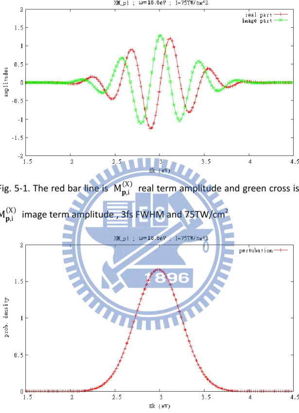
M_𝐩,i X real and image term amplitudes and probability density in Fig. 5-1. and Fig. 5-2.

16

Fig. 5-1. The red bar line is M_𝐩,i X real term amplitude and green cross is M_𝐩,i X image term amplitude , 3fs FWHM and 75TW/cm2

Fig. 5-2. The red bar line is M_𝐩,i X probability density with photoelectron energy. The laser pulse use 3fs FWHM and 75TW/cm2

17

With M_𝐩,i(X) and M_2p,i(X) obtained, the time evolution of the electronic wave packet can be easily obtained. In an experiment, of course the goal is to apply a probe pulse at different time delays from which information about this wave packet can be uncovered. We note that the whole electron wave packet actually includes the contribution from the 1s part. However, the 1s state is energetically well separated from the 2p and the continuum electrons, we can use a low-energy probe pulse without perturbing the 1s part of the wave packet.

For the one-photon absorption by the probe pulse, first-order perturbation theory gives

M_𝐩,2p(L) = −i dt τ+τ₂L τ−τ₂L e−i(ϵ2p−ϵ𝐩) t− τ− 𝜏_𝐿 2 _Ψ𝐩− r ϵ ∙ r E_L t − τ ϕ 2p r (5.10) M_𝐩,2p(L) also with the gaussian E t = ϵ Em ∙ e

−2ln 2

Δ2 t 2

∙ cos ωt + ϕ_p the CEP phase ϕ_p can be set 0 , too. The polarization ϵ is also along z-axis. For hydrogen from ground state to continuous state of incoming boundary condition, for pulse in τ −τL

2 , τ + τL

2

Use the same method

M_𝐩,2p(L) = −1 l_ei σl−𝜏₂𝐿 ϵ𝐩−ϵ2p +ϕp _E m πΔ2 8ln2∙ e − ϵ𝐩−ϵ2p−ω 2 Δ2 8ln 2 _{∙ 𝐩 ϵ ∙ r ϕ} 2p r (5.11) 𝐩 ϵ ∙ r ϕ_2p r = REl∗ r Ylm ∗ Ωr Ylm Ωk l m=−l ∞ l=0 4π 3 Y1 0_{(r ) ∙ r ∙ R} 21 r Y10(r ) ∙ r2dΩdr (5.12) Y₁0 r Y₁0 _{r =} 3 4πcos 2_{θ =} 3 4π 1 3 3cos 2_{θ − 1 +}1 3 = 3 4π 4 3 π 5Y2 0₊ 4π 3 Y0 0 (5.13)

18 𝐩 ϵ ∙ r ϕ_2p r = 4 15Y2 0 _Ω k RE2∗ r R10 r ∙ r3dΩdr + 1 4πY0 0 _Ω k RE0∗ r R10 r ∙ r3dΩdr = 1 12π 3cos 2_θ k− 1 RE2∗ r R10 r ∙ r3dΩdr + 1 4π RE0 ∗ _{r R} 10 r ∙ r3dΩdr (5.14) R_E2 and R_E0 are also solve by Numerov method.

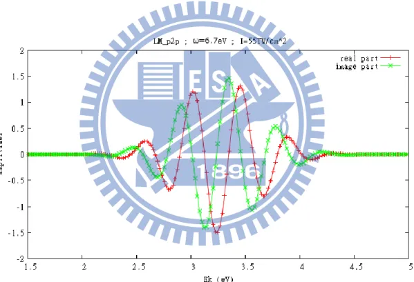
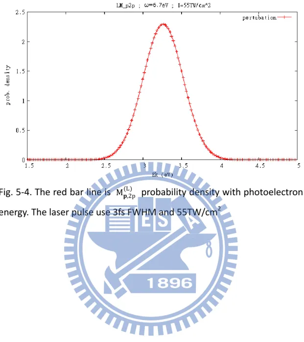
As well as , M_𝐩,2p(L) real and image term amplitudes and probability density in Fig. 5-3. and Fig. 5-4. .

Fig. 5-3. The red bar line is M_𝐩,2p(L) real term amplitude and green cross is

19

Fig. 5-4. The red bar line is M_𝐩,2p(L) probability density with photoelectron energy. The laser pulse use 3fs FWHM and 55TW/cm2

20

6. Results

When get the transition amplitudes M_𝐩,2p(L) ,M_2p,i(X), and M_𝐩,i(X) ,than combine to find M_𝐩i(τ) 𝟐 in Fig. 6-1. and Fig. 6-2.

Fig.6-1. Photoelectron energy spectrum M_𝐩i(τ) 𝟐 (blue star line) obtained by θk=45° and time-delay τ =

τL

2 + τx

2 with M𝐩,i (X) 2

(red bar line) and M_2p,i(X) M_𝐩,2p(L) 2(green cross line)

21

Fig.6-2. Photoelectron energy spectrum M_𝐩i(τ) 𝟐 (blue star line) obtained by θk=45° and time-delay τ =

τL 2 + τx 2+1 with M𝐩,i (X) 2 (red bar line) and M_2p,i(X) M_𝐩,2p(L) 2(green cross line)

The interference in the angular distribution in Fig.6-3. can be understood from the angular momentum components of the photoelectrons.

22

Fig.6-3. Angular distribution of photoelectron for a fixed energy ϵ=3.1eV at several delay-times. Here τ = τL

2 + τx 2 + Td so Td = τL 2 + τx 2 + τ

For the narrow energy range where the electron yields are large, we can expect all the other parameters are nearly energy independent, thus the peaks of the spectra occur when

Φ_𝐩,2p − (ϵ_𝐩− ϵ_2p)τ = 2nπ

where n is a positive or negative integer. This equation shows that the peak shall follow a hyperbola with the peak shifts to smaller τ for larger ϵ. Thus the hyperbola is tilted toward smaller τ for larger ϵ (and larger τ for smaller ϵ). The tilt is more toward the horizontal axis as τ increases. These general features can be clearly seen in Fig.6-4. and Fig.6-5.

23

Fig.6-4. Interferogram forθ k=π depend on time-delay τ .

Fig.6-5. Interferogram for fix time-delay τ =τL

2 + τ_x

2 and depend on

24

7. Conclusion

The model of pump-probe process using by pump and probe laser. The pump process combination by two step. First, using laser for bound-bound excitaion (from 1s to 2p),and second 1st-order perturbation for bound (2p) to continuum state.

The probe pulse also have two effects. First, the continuous wave packet is Volkov like, time-delay τ=0 with Gaussia pulse. 1s2p + laser calculated by 1st-order perturbation.

The interferogram show by hyperbola and peaks of the spectra occur when Φ𝐩,2p − (ϵ𝐩− ϵ2p)τ = 2nπ , which in the ionization

25

Reference

[1] X.M. Tong and C.D. Lin, J. Phys. B38, 2593 (2005).

[2] See for example, S. Gasiorowicz, Quantum Physics, 2nd ed. Chapter 21 (John-Wiley & Sons, New York,1996).

[3] Anh-Thu Le,R.R. Lucchese, S. Tonzani, T. Morishita, and C. D. Lin, Phys. Rev.A80, 013401 (2009).

[4] Louis H. Haber, Benjamin Doughty,and Stephen R.Leone, Phys. Rev. A79,031401R (2009).

[5] F. Kelkensberg et al., Phys. Rev. Lett. 103, 123005 (2009). [6] J. L. M. Quiroz González and D. Thompson

26

Appendix Atomic units

Atomic units (au) form a system of units convenient for atomic physics, electromagnetism, and quantum electrodynamics, especially when the focus is on the properties of electrons.

In au, the numerical values of the following four fundamental physical constants are all unity by definition:

Electron mass : me = 1

Elementary charge : e = 1

reduced Planck's constant : ℏ = 1 (1) Unit of change = change of electron = |e| =1.602 x 10-19 C (2) Unit of mass = mass of electron = me =9.109 x 10-31 kg

(3) Unit of length = radius of ground state = 1 bohr

= 0.53 x 10-10 m = 0.53 Å

(4) Unit of time = period of ground state electron orbiting = _Va 0 = ℏ3 me4 = 2.42 x 10 -17 s (5) Unit of velocity = speed of electron = e2

ℏ = 2.2 x 10 8

cm/s = αc = _137.037c

(6) Unit of angular frequency = V_a0 = 4.1 x 1016 s-1 (7) Unit of energy = e2

a = 1 Hartree = 2 Rydberg = 27.2 eV

(8) Unit of electric field = e

a2 = 5.14 x 10

9 _Volt/cm

α: fine structure constant = e_ℏc2 = 1

137.037

27

Laser intensity in vacuum I = time averaged laser intensity

= _4πc E2

= 137.037_4π ∙ E2

= 7.0192 x 1016 ∙ E2 W/cm2

E = _{7.0192 x 1016}I a.u.

1 a.u. ( intensity ) = 1 Hartree

1 a.u.time a2

= _{2.42 x 10−17}4.36 x 10 _{s 0.53 x 10}−18 J _{−8 cm 2} = 6.44 x 1015 W/cm