穩健性腦磁波訊號源造影

國

立

交

通

大

學

多媒體工程研究所

碩

碩

碩

碩

士

士

士

士

論

論

論

論

文

文

文

文

穩 健 性 腦 磁 波 訊 號 源 造 影

Robust Magnetic Source Imaging of Brain Activities

研 究 生：楊令琤

指導教授：陳永昇 博士

中

中

中

研 究 生：楊令琤 Student：Ling-Cheng Yang

指導教授：陳永昇 Advisor：Yong-Sheng Chen

國 立 交 通 大 學

多 媒 體 工 程 研 究 所

碩 士 論 文

Submitted to Institute of MultimediaEngineering College of Computer Science

National Chiao Tung University in partial Fulfillment of the Requirements

for the Degree of Master

in

Computer Science

August 2007

Hsinchu, Taiwan, Republic of China

To discover brain functionalities, we need to do brain source imaging. Magnetoen-cephalography (MEG) can record brain signals non-invasively with superior temporal res-olution and high Signal-to-Noise Ratio (SNR).

There are some issues about magnetic source imaging, like the amount of MEG record-ings, the appropriate approach for signal analysis and source localization and head motion correction. We propose some methods to overcome these difficulties. First, we use statis-tical hypothesis test to reveal the discrimination between the selected active and baseline states. By revealing their discrimination, we can set an evaluation criterion for the amount of recordings.

Second, in order to conduct signal analysis, Independent Component Analysis (ICA) is an powerful method which can retrieve independent components from the linear mixture of sources, under the assumption that components are statistical independent. However, the resolution of ICA topography distribution is in sensor space. If we want to achieve the goal of source imaging, it is necessary to raise the resolution to tomography distribution in source space .

Many algorithms are proposed to solve the problem of source localization. In recent years, the most attracting method is Beamforming. It can obtain the activation magnitude of the targeted source by imposing the unit-gain constraint while suppressing the contribu-tion from other sources by applying the minimum variance criterion. Maximum Contrast Beamformer (MCB) is an outstanding method that it can estimate the orientation of the spatial filter from an analytical form which is generated from maximizing the contrast of active state and control state. However, the major problems in beamformer are the parame-ters needed to be well-selected, especially the regularization parameter. The inappropriate value of the regularization parameter can result in inaccurate spatial filter estimation.

We get more accurate solution to source localization by combining ICA with MCB, which is called Beamformer-based ICA. We consider filtered signals form the MCB spatial filter as the output from the virtual sensor at each voxel of interest and take them as the ICA input signals. As a result, with inappropriate regularization parameter of beamfermer, we can use ICA to separate leakage from target source. Furthermore, we can raise ICA

Third, there are still some factors that will affect the accuracy of source localization, like the head motion during MEG experiments. This is unavoidable during MEG studies with long signal recording time. Many algorithms are proposed to solve this problem. With Stabilized Linear Model (SLIM), we can virtually increase the sensor number of MCB model to reduce the localization error induced from head motion and improve the accuracy of source localization simultaneously.

Experiments with simulation and real data are used to validate the proposed methods. According to the experiments, by revealing the discrimination between the selected active and baseline states, we can set an evaluation criterion for the amount of recordings. More-over, as aforementioned, the expected advantages of Beamformer-based ICA are demon-strated with simulation data. Applying SLIM into MCB is also validated that it is able to reduce the localization error induced from head motion and improve the accuracy of source localization by combining the different head poses.

為了探索人腦功能，腦部訊號源造影是必須的。腦磁波儀可以非侵入式地量 測腦波訊號，並且具有優越的時序解析度和高訊雜比。我們可以藉由腦磁波儀所 提供的腦波訊號時間及空間資訊來達到腦部功能探索的目的。 腦部訊號源造影有很多相關的議題，例如腦磁波儀所擷取到的腦波訊號量、 何者為適當的訊號分析以及訊號源造影、以及一些影響訊號源估測的因素。我們 提出了一些方法來解決上列的問題。首先，我們利用統計檢定的方法，顯示活化 狀態和控制狀態的差異性。藉由顯示兩者的差異程度，當達到顯著差異的感應器 數量夠多時，我們可以得到一個判斷擷取到的訊號量已經足夠的依據。 第二，為了達到訊號分析的目的，獨立成分分析是一個很強大的方法，它可 以將線性組合的訊號分解成獨立成分。然而，用獨立成分分析時，我們通常會觀 察每個獨立成分的時序活動狀態和腦部地形圖的分佈狀態。當輸入訊號是腦磁波 儀量測到的腦波訊號時，腦部地形圖的解析度就會是在感應器層，我們希望提升 到斷層掃瞄的解析度。 許多演算法被提出來為了解決訊號源位置估測的問題。以光束構成法為基礎 之空間濾波法進行腦磁波活動源估測近年來受到矚目。此法主要的優點在於針對 某一位置估算其腦部活動訊號時，能在維持其活動強度的條件下同時抑制其他訊 號源對估算所產生的影響。以最大對比為限制之改良式腦磁波光束構成法是一個 新穎的方法，利用最大化活化狀態和控制狀態的變異數之對比估算出一個空間濾 波器的最佳方向。但是光束構成法最大的問題就是有很多需要調整的參數，尤其 是正規化參數。不適合的正規化參數會導致不準確的空間濾波器。 我們結合了獨立成分分析和以最大對比為限制之改良式腦磁波光束構成 法，稱之為以光束構成法為基礎的獨立成分分析。將以最大對比為限制之改良式 腦磁波光束構成法得到的空間濾波器濾出的訊號當作獨立成分分析的輸入訊 號。因此，一些因為不適合的正規化參數所造成的漏電流，可以藉著獨立成分分 析將其分離。再者，我們可以藉由光束構成法之虛擬感應器的觀念來提升獨立成 分分析的結果達到斷層掃瞄的解析度。 第三，仍然有一些會影響訊號源位置估測的因素，例如在腦磁波儀實驗中的 頭部移動，很多演算法提出來為了解決這個問題。其中穩定線性模型不僅可以解 決頭部移動的問題，同時也因為具有虛擬增加感應器的能力而提升了訊號源位置 估測的正確性。 模擬訊號、假體和實際實驗的訊號同時用來檢測以上方法的正確性。我們使 用配對 t 統計來檢測活化和控制狀態訊號的差異度，藉由這個結果，我們可以設 定一個評估訊號量是否足夠的準則。再者，以光束構成法為基礎的獨立成分分析 的優點也經由實驗被證實。最後，將穩定線性模型套入以最大對比為限制之改良 式腦磁波光束構成法，的確可以解決頭部移動的問題；並藉由結合各種不同頭部 位置的訊號，虛擬地增加感應器數量，而得到更準確的訊號源位置估測結果。

在兩年的碩士生涯中，我要感謝很多人給予的鼓勵與幫助。首先是兩位指導 老師，陳永昇老師與陳麗芬老師，在兩年多來給予我許多研究上的幫助，不僅提 出許多寶貴的意見來引導我做研究，也會適時地給予關心。更要感謝默默支持我 的父母和姊姊，即使我不常回家，但他們仍舊不時地關心我的近況，也不斷為我 加油打氣。也要感謝實驗室的同學和我身邊所有支持鼓勵我的朋友，可以陪我聊 天、打球、玩樂，與我分享我的快樂與難過。最後也要謝謝我的男朋友，感謝他 一路支持我，照顧我，給我溫暖。感謝所有幫助過我的人讓我能順利從交大畢業， 謝謝你們。

A dissertation presented

by

Ling-Cheng Yang

to

Institute of Multimedia Engineering

in partial fulfillment of the requirements

for the degree of

Master of Science

in the subject of

Computer Science and Information Engineering

National Chiao Tung University

Hsinchu, Taiwan

Copyright © 2007 by

List of Figures v

List of Tables vii

1 Introduction 1

1.1 Related Works of Magnetic Source Imaging . . . 2

1.1.1 Amount of Recordings . . . 5

1.1.2 Signal Analysis and Source Localization . . . 5

1.1.3 Head Motion Correction . . . 17

1.2 Thesis Scope . . . 18

1.3 Thesis Organization . . . 18

2 Robust Magnetic Source Imaging 21 2.1 Statistical Evaluation of the Amount of Recordings . . . 22

2.1.1 Statistical Hypothesis Test . . . 22

2.1.2 Evaluation of the Amount of Recordings with Statistical Hypothe-sis Test . . . 23

2.2 Beamformer-based ICA . . . 27

2.3 Head Motion Correction . . . 31

2.3.1 Stabilized Linear Model . . . 31

2.3.2 Solutions to Inverse Problem with Maximum Contrast Beamformer 32 3 Experiment Results 35 3.1 Material . . . 36

3.2 Data Preprocessing . . . 40

3.3 Statistical Evaluation of the Amount of Recordings . . . 42

3.4 Beamformer-based ICA . . . 45

3.5 Head Motion Correction . . . 50

3.5.1 Simulations . . . 50

3.5.2 Phantom . . . 50

3.5.3 Experiment of Gender Discrimination . . . 54

4.2 Practical Issues of Beamformer-based Independent Component Analysis . . 61 4.3 Sensor Number Issue of MEG . . . 61

5 Conclusions 65

Bibliography 67

1.1 MEG Device at Taipei Veterans General Hospital. . . 3

1.2 Effect of whitening. . . 8

1.3 ICA algorithm. . . 9

1.4 The concept about unit-gain and minimum variance constraints in beam-former. . . 12

1.5 The filtered source power with beamformer spatial filter. . . 13

1.6 Maximum Contrast Beamformer. . . 16

1.7 Solution to the inverse problem calculated by MCB algorithm. . . 16

1.8 Head fixing during MEG experiments. . . 17

2.1 Beamformer-based ICA algorithm. . . 30

2.2 Concept of stabilized linear model. . . 33

3.1 The device of MEG phantom. . . 37

3.2 The configuration of MEG phantom. . . 38

3.3 Experimental paradigm of gender discrimination. . . 38

3.4 Preprocessing for MEG recordings. . . 41

3.5 Statistical analysis of average recordings. . . 43

3.6 Statistical analysis of raw recordings. . . 44

3.7 Ground truth of the simulated recordings for Beamformer-based ICA. . . . 46

3.8 Ground truth of the simulated recordings for SLIM. . . 51

3.9 F-statistical map of simulated recordings when the value of α is 0.0003. . . 52

3.10 F-statistical map of simulated recordings when the value of α is 0.0008. . . 52

3.11 Localization error evaluation among the SLIM and Averaging. . . 53

3.12 Visual pathway. . . 54

3.13 Topography and waveform (leaning backward). . . 57

3.14 Topography and waveform (leaning forward). . . 58

2.1 List of statistical hypothesis tests for testing the difference in mean . . . 26

3.1 Experimental stimuli. . . 39 3.2 The result of Beamformer-based ICA when the regularization parameter of

0.0003. . . 47 3.3 Beamformer-based ICA when the regularization parameter of 0.003. . . 48 3.4 List of localization error evaluation among the SLIM and Averaging. . . 53 3.5 Results of MCB and SLIM with different head poses and the control state

is set as 800 ms to 1000 ms. . . 55 3.6 Results of MCB and SLIM with different head poses and the control state

is set as the empty room recordings. . . 56

4.1 Beamformer-based ICA when the regularization parameter of 0.03. . . 62

1.1

Related Works of Magnetic Source Imaging

For Human beings, brain is the most important component to coordinate all parts of our body. For thousands of years, people have devoted themselves to discover the accurate brain functionalities. With the progress of the technologies, invasive anatomy becomes non-invasive functional brain mapping, that ”non-invasive” means without physical harm. In order to acquire brain signals non-invasively, we can measure electrophysiological, hemodynamic, metabolic, and etc. Recently, Magnetoencephalography (MEG), Electroen-cephalography (EEG), functional Magnetic Resonance Imaging (fMRI) and Near-Infrared Reflectance Spectroscopy (NIRS) are four major modalities.

When neurons become active, they induce changes in blood flow and oxygenation lev-els, which can be imaged related to neural activity. fMRI can detect hemodynamic changes with spatial resolution as high as 1-3mm. However, because of the relatively slow hemo-dynamic changes, fMRI has relatively poor temporal resolution (in the order of seconds) compared with techniques such as EEG and MEG.

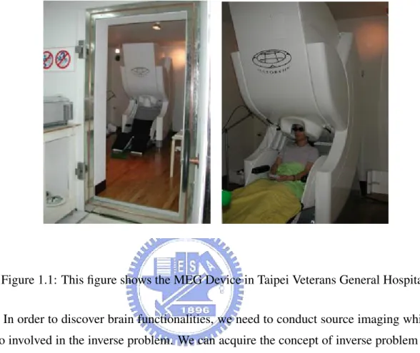
MEG and EEG are two complementary techniques that measure the magnetic induction and the scalp electric potentials produced by the ensemble of neuronal activities inside the brain. The major advantage of MEG and EEG is the higher temporal resolution (in the order of milliseconds) compared to fMRI, because they measure electrical brain activity directly. Furthermore, MEG is an imaging technique which measures the magnetic fields produced by electrical activities inside the brain via extremely sensitive devices such as superconducting quantum interference devices (SQUIDs) which has higher signal-to-noise ratio (SNR) than EEG. Therefore, MEG is often used as the modality for source imaging. However, the spatial resolutions of EEG and MEG are limited for two reasons. One is the limited number of spatial measurements. EEG and MEG measure brain signal with limited electrodes or sensors, usually tens or a few hundreds. Compared to fMRI, tens of thousands, that’s relatively a small amount. The other reason is the inherent ambiguity of the inverse problem, finding the distribution of sources when the recordings are given. Even with infinite MEG and EEG sensors, a non-ambiguous solution to localization of the neuronal activity inside the brain would not be possible. We can reach similar resolutions to those of fMRI only by adding restrictive models on the sources of MEG and EEG signals [1]. We

can see the MEG device in Figure 1.1.

Figure 1.1: This figure shows the MEG Device in Taipei Veterans General Hospital.

In order to discover brain functionalities, we need to conduct source imaging which is also involved in the inverse problem. We can acquire the concept of inverse problem from the Bayesian statistic framework.

P (x|y) = P (x)P (y|x)

P (y) (1.1)

P (x|y) is the conditional probability of x, given y. It is also called the posterior proba-bility because it is derived from or depends upon the specified value of y. P (y|x) is the conditional probability of y given x. P (y) is the prior or marginal probability of y, and acts as a normalizing constant. P (x) is the prior probability or marginal probability of x. It is ”prior” in the sense that it does not take into account any information about y. Applying the Bayesian statistic framework to MEG inverse problem and let x represent the distribution of the sources in the head and y represent the recordings from the MEG sensors. P (x|y) can describe the inverse problem that to get the distribution of the sources while given MEG recordings. From the Bayesian equation, we can simplify the inverse problem as the form

of the right side of the equal sign if we want to know parameters of the source distribution from the recordings. Therefore, P (y|x) is the key to the solution. P (y|x) describes the probability of the recordings when given parameters of the source distribution and that is the forward problem.

However, there are many difficulties of robust source imaging, like the amount of MEG recordings, the appropriate approach for signal analysis and source localization and head motion correction. First, we discuss about the amount of recordings. For robust source imaging, we need large enough SNR of recordings and SNR can be enhanced with suffi-cient number of acquired trials. Because there are no explicit criteria or rules for experi-mentalist to follow, the number of recordings is always determined with the experimental-ist’s rule of thumb. This is very subjective.

Even the amount of recordings is enough for data analysis, what is the appropriate ap-proaches for source analysis and localization is another important issues. To signal analysis, Independent Component Analysis (ICA) is an powerful method that can retrieve indepen-dent components from the linear mixture of sources, under the assumption that components are statistical independent. There are many algorithms proposed to solve the problem of source localization. Source localization is an ill-posed problem because the number of sources is much larger than the number of the sensors, additional constraints are necessary to solve this problem. Among the approaches for source localization, beamformer is more focal and accurate. Therefore, beamformer is the most attracting method in recent years.

There are still some situations that will affect the accuracy of source localization, like the head motion during MEG experiments. If there is head motion during experiments, the relative position between head and sensors will be changed and induce errors of source localization. However, to MEG studies, head motion during MEG experiments is unavoid-able in the long signal recording time. We need to solve this crucial problem for higher accuracy of source localization.

1.1.1

Amount of Recordings

To get event-related potential for signal analysis and source localization, we usually need tens or hundreds of trials of brain signals for large enough SNR. To our knowledge, there is still no on-line evaluation method in the literature to realize whether the amount of MEG recordings is enough.

The easiest way is the visual inspection of on-line averaged waveform. While the ex-pected (or well-known) features of averaged waveform exist, we can determine that the amount of recordings is enough. But this is a subjective method and what we need is an objective formal criterion.

For some methods of statistical thresholding of source activities, they extract target source activities by comparing the discrimination between the target and non-target source activities [2, 3]. Following this concept, in this thesis, we display the discrimination be-tween the selected active and control states from MEG recordings to give the experimen-talist a concept about the amount of recordings and saves the unnecessary time and effort.

We use statistical hypothesis test to get this discrimination.

1.1.2

Signal Analysis and Source Localization

Signal Analysis

For signal analysis, ICA is an powerful method. Originally, ICA is proposed to solve the problem of blind source separation. In the following statements, we express the concept of ICA.

We want to recover N independent source signals s = {s1(t), . . . , sN(t)} after they are

linearly mixed by a mixing matrix A.

x = {x1(t), . . . , xN(t)} = As (1.2)

Given x, we will estimate an unmixing matrix W which can recover x to original sources u = Wx under the assumption that the estimated sources u are as statistically independent as possible. Here u contains independent components.

In advance, we should know that uncorrelated is not independent. Independence is a stronger constraint than uncorrelation. Two random variables are said to be uncorrelated if

their covariance is zero.

E{y1y2} − E{y1}E{y2} = 0 (1.3)

If the random variables are independent, they are uncorrelated. However, that the random variables are uncorrelated cannot imply they are independent. Take sin(x) and cos(x) for example, they are both dependent on x, but they are uncorrelated since cov(sin(x), cos(x)) = 0. Moreover, uncorrelatedness is a relation between only two random variables, whereas independence can be a relationship between more than two random variables.

Decorrelation methods, like PCA can give uncorrelated output components. While PCA decorrelates the outputs, ICA attempt to make the outputs statistically independent.

First, we should know that there are some assumptions in ICA [4].

I. The independent components are assumed to be statistically independent.

This is the main assumption that ICA requires. We say that random variables y1, y2, . . . , yn are independent if the information of yi does not give any

informa-tion of yj for all i 6= j. To represent this concept as a mathematical form, we can

formulate it as the form of probability density function.

p(y1, y2, . . . , yn) = p1(y1)p2(y2) . . . pn(yn) (1.4)

where p(y1, y2, . . . , yn) is the joint probability density function of yiand pi(yi) is the

marginal probability density function of yi.

II. Gaussian variables are forbidden.

The order cumulants for gaussian distribution are zero, but such higher-order information for estimation of the ICA model is necessary. One can prove that the distribution of any orthogonal transformation of gaussian random variables gives exactly the same information. Thus, in the case of gaussian variables, we can only estimate the ICA model up to an orthogonal transformation. In other words, the matrix is not identifiable for gaussian independent components. (Actually, if just one of the independent components is gaussian, the ICA model can still be estimated.)

Second, there are some ambiguities in the ICA algorithm. We explain it in the below statements:

I. The variances of independent components are unknown.

We cannot determine the variance of the independent components. Because both A and s are unknown, any scalar multiplier in one of the sources siof s could always

be canceled out by dividing the corresponding column ai of A by the same scalar.

II. The order of the independent components is unknown.

We cannot determine the order of the independent components. We can always apply a permutation matrix P to Eq (1.2), x = AP−1Ps. Then Ps is still like the original signals and AP−1 is just a new unknown mixing matrix and can also be solved by ICA algorithm.

Since we have got the concept from ICA and understood its assumptions, we should go on for its optimization algorithm. The major concept is that to make the output component as statistically independent as possible. This leads to another problem about how to mea-sure the independence. We should know in advance that non-gaussian is independent. By the central limit theorem (CLT), the distribution of a sum of independent random variables tends toward a gaussian distribution. In other words, the mixing of two independent signals usually has a distribution that is closer to gaussian distribution than any of the two original signals. From this concept, u = Wx = WAs that u must be more gaussian than s because of CLT. But we want u is a copy of s so that u must be the least gaussian. That equals to maximize the non-gaussianity of Wx.

Usually kurtosis is used as a measure of the non-gaussianity. The kurtosis of a gaussian random variable is zero. But existing a problem about kurtosis that it is very sensitive to outliers. As a result we use the negentropy to replace the kurtosis. From the information theory, a gaussian variable is that it has the largest entropy among all random variables. We can take the entropy as a measure of non-gaussianity. For computation simplicity, we use an approximation to calculate the negentrophy.

J (u) ≈ c[E{G(u)} − E{G(ν)}] (1.5)

where c is some constant, E is the expectation value, ν is a gaussian variable of zero mean and unit variance and G is a non-quadratic function, called a contrast function. There are some choices about G, like tanh, exp and the power function [5].

In ICA algorithm, the contrast function G is a parameter that we should choose for every different condition [5]. Furthermore, we need to do preprocessing to make the problem of ICA estimation simpler and better conditioned. Whitening is a preprocessing step that can make the input x uncorrelated and unit variance. We can see that the effect of the whitening processing in Figure 1.2. Figure 1.2 (a) is the joint density function of original independent signal with uniform distribution. After uncorrelated mixtures of the independent signals, the distribution is as Figure 1.2 (b), is no more independent. Figure 1.2 (c), we can see the effect of whitening that the square defining the distribution is now clearly a rotated version of the original square in Figure 1.2 (a). Whitening can be achieved with principal component analysis (PCA) or singular value decomposition (SVD).

(a) (b) (c)

Figure 1.2: This graph shows the effect of whitening. (a) is the joint probability density function of original independent signal with uniform distribution. (b) is the distribution after uncorrelated mixtures of the independent signals from (a). (c) is the joint distribution of the whitened mixtures.

We can have an overview of ICA algorithm in Figure 1.3. The first step is whitening to make the problem of ICA estimation simpler and better conditioned. The second is to optimize the un-mixing matrix W iteratively by maximizing the non-gaussianity, approxi-mated by calculating the negentrophy with the contrast function G. This optimization step can reach the purpose of ICA, making the output components as statistically independent as possible.

whitening estimate W input measurementx un-mixingmatrix W optimization maximizethe non-gaussianity

Figure 1.3: This graph shows the overview of ICA algorithm. The first step is whitening to make the problem of ICA estimation simpler and better conditioned. The second is to optimize the un-mixing matrix W iteratively by maximizing the non-gaussianity.

etc. All of them have some advantages and disadvantages. Since we want to solve the problem efficiently, we choose FastICA [5, 6] algorithm as our method.

Source Localization

As aforementioned, because the electromagnetic field recorded by MEG sensors is the ensemble of neuronal activities within the whole brain, we can determine the recorded electromagnetic field from forward solutions. Therefore, the inverse problem can be trans-formed to estimate the neuronal activities inside the brain by Eq 1.1. But these inverse problems are ill-posed problems because the number of sources is much larger than the number of the sensors, additional constraints are necessary. A lot of algorithms had been proposed [1] to solve the inverse problem.

The most widely-used method is least square dipole fitting [7, 8]. It assumes the neu-ronal activities are composed of a fixed number of Equivalent Current Dipoles (ECD) and

finding out the best solution by minimizing the error between the electromagnetic field generated by ECDs and by MEG/EEG recordings. However, two difficulties of this al-gorithm are a priori number of sources and trapping in local minimum. Multiple Signal Classification (MUSIC) [9–11] is another kind of method. It can avoid trapping in local minimum by searching through the region of interest and determining the locations with peak projections of forward models in the signal subspace. Because there is no perfect head model and MEG/EEG recordings, how to determine the best signal subspace is an impor-tant issue. Minimum Norm Estimation (MNE) [12] will set dipole orientation either to be on the tangential plane or normal to the local cortical surface. But the major problem is that because of the minimum norm constraint, the result will tend to emphasize the cortical regions closer to the MEG sensors.

The most attracting method for inverse problem in recent years is Beamforming [13,14]. We can think that the beamformer creates a virtual sensor at a specified position in the source space by the information recorded from MEG sensors to measure the signals with a specified orientation. It can obtain the activation magnitude of the targeted source by imposing the unit-gain constraint while suppressing the contribution from other sources by applying the minimum variance criterion. This property can improve the spatial resolution and the accuracy of the spatial filter.

There are two kinds of Beamformer, vector-type beamformer [15] and scalar-type beam-former [16]. The vector-type beambeam-former decomposes the dipole into three orthogonal components. Every component has its own spatial filter. There is only one spatial filter in scalar-type beamformer and it determines the direction by maximizing the Z-value. Com-pared to scalar-type beamformer, it is more efficient to calculate the spatial filter by using vector-type beamformer because all the involved procedures are deterministic. But the ma-jor advantage of scalar-type beamformer is the higher Signal-to-Noise Ratio (SNR) and higher spatial resolution [17, 18].

We can think that the beamformer creates a virtual sensor at a specified position in the source space by the information recorded from MEG sensors to measure the signals with a specified orientation. There are two types of beamformers, vector-type [15] and scalar-type beamformer [16]. The scalar-scalar-type and vector-scalar-type beamformer give exactly the same output power and output SNR when the orientation is optimum. However, the theoretical

output SNR of a vector-typed beamformer is significantly degenerated without optimum orientation [17].

We describe the theorem of scalar beamformer in the below statements.

I. Scalar Beamformer

First, involving Sarvas forward model [19–21], the MEG recordings can be writ-ten as considering a target unit dipole with parameter θ = {rq, q} where rq is the

dipole location and q is the dipole orientation. We can further separate m(t) into three components

m(t) = mθ(t) + mδ(t) + n(t) (1.6)

where mθ(t) denotes the contribution from target source, mδ(t) denotes the

mag-netic recordings generated from all other sources and n(t) denotes the noises in real environment. While merging mδ(t) + n(t) into mn(t) and replacing the mθ(t) with

the form of lead filed, the above equation becomes

m(t) = lθsθ(t) + mn(t) (1.7)

sθis the dipole moment and lθ is the lead field which means the predicted recordings

of the unit dipole with q orientation.

Here lθis the combination of lead field matrix Lrand dipole orientation q,

lθ = Lrq (1.8)

The output signal y(t) can be formulated by filtering the MEG recordings with the spatial filer wθ, denoting by

y(t) = wθtm(t) (1.9)

We further apply Eq (1.7) into Eq (1.9). We can get the concept about unit-gain and minimum variance constraints from Figure 1.4. With unit-gain constraint, the spatial filter at the location of the target source (r, q) will preserve the most strength and impress the contribution form other sources by minimum variance constraint.

wT_l=1

wT_{l=0 r,j}

Figure 1.4: With unit-gain constraint, the spatial filter at the location of the target source(r, q) will preserve the most strength and impress the contribution form other sources by minimum variance constraint.

Therefore, we can write the formula as:

y(t) = wθtm(t)

= wθtmθ(t) + wθtmn(t)

= sθ(t)wθtlθ+ wθtmn(t)

= sθ(t) + wθtmn(t) (1.10)

From the above, in order to approximate the output signal y(t) as source strength sθ, we must suppress the leakage of sources from other locations, wθtmn(t),

corre-sponding to minimize variance of y(t). Therefore, we can obtain the optimal spatial filter from

ˆ

wθ = arg min wθ

E{ky(t) − E{y(t)}k2} + αkwθk2 subject to wθtlθ = 1 (1.11)

where E represents the expectation value and α represents the parameter of Tikhonov regularization [22]. Here α is a parameter to adjust the tradeoff between specificity and noise sensitivity, corresponding to the shape of beamformer spatial filter.

Substituting the equation Eq (1.10) into Eq (1.11), we can solve this equation by Lagrange multipliers then get the solution to wθ:

ˆ wθ = arg min wθ wθt(C + αI)wθ subject to wθtlθ = 1 = (C + αI) −1_l θ lθt(C + αI)−1lθ (1.12)

where C is the covariance matrix of the MEG recordings m(t) and I is the NxN identity matrix.

II. Statistical Mapping

Because the SNR of the recordings is often small, the effect from the non-task-related sources is necessary to be considered. At every target position rq, we can get

the spatial filter from Eq (1.12). The norm of the spatial filter is location-dependent. The lead field norm of a deeper source is bigger than that of a superficial source and because of the unit-gain constraint, the norm of spatial filter is inversely-squared-proportional to the norm of the lead field. Therefore, if we take only the filtered source power as the measure of the source distribution may contain strong non-task-related source distribution. This phenomenon is shown in Figure 1.5. If we display only the filtered source power, the power variance will focus on the deep part within the brain (Figure 1.5 (a)). We can reduce this problem by normalizing the filtered source power with the noise [15] (Figure 1.5 (b)).

Figure 1.5: (a) is the filtered source power with beamformer spatial filter. The power variance will focus on the deep part within the brain. (b) is the result of normalizing the filtered source power with the noise. The problem is reduced clearly in the figure. [17]

Fθ = E{kwθtma(t) − E{wθtma(t)}k2} E{kwθtmc(t) − E{wθtmc(t)}k2} = wθ t_C awθ wθtCcwθ (1.13)

where Cais the covariance matrix estimated from the MEG recordings in active state

ma and Cc is the covariance matrix estimated from the MEG recordings in control

As a result, the value of Fθ represents that at the target location rq with orientation

q, the probability of existing a statistically significant brain activity. By F-statistical map of MCB, we can get the solution to the inverse problem.

III. Maximum Contrast Beamformer

There is a parameter θ in Eq (1.12) needed to be estimate in advance. If we can estimate θ more accurately, the spatial filter will be closer to optimum. Instead of the exhaustive search or the sub-optimal nonlinear search, a newly-proposed method, Maximum Contrast Beamformer (MCB) [23], has the very outstanding advantage. It can estimate the orientation of the spatial filter from an analytical form which is generated from the criterion that maximizing the variance of active state and control state, and preserve the advantage of scalar-type beamformer simultaneously. Effi-ciency and accuracy are the most attracting properties of MCB.

In order to estimate an optimum dipole orientation in analytical form, first we substi-tute Eq (1.8) into Eq (1.12) to separate the dipole orientation q, then

ˆ wθ = (C + αI)−1Lrqq qt_Lt rq(C + αI) −1_L rqq = Arqq qt_B rqq where Arq = (C + αI) −1 Lrq and Brq = L t rqArq (1.14)

Then substituting Eq (1.14) into Eq (1.13) and maximizing the value of F-statistic, we get ˆ q = arg max q (_qAt_Brqq rqq) t_C a( Arqq qt_B rqq) ( Arqq qt_B rqq) t_C c( Arqq qt_B rqq) = arg max q qt_At rqCaArqq qt_At rqCcArqq = arg max q qtPrqq qt_Q rqq (1.15)

where Prq = Arq

t

CaArq and Qrq = Arq

t

CcArq

The solution to ˆq in Eq (1.15) is the eigenvector corresponding to the maximum eigenvalue of the matrix Q−1_rqPrq.

After replacing Arqand Brq into Prqand Qrq, we can get

Prq = Lrq t_{(C + αI)}−t_C a(C + αI)−1Lrq (1.16) Qrq = Lrq t_{(C + αI)}−t_C c(C + αI)−1Lrq (1.17)

An overview process of MCB is shown in Figure 1.6. With MEG recordings and the control state, the active state and the regularization parameter are well-selected, we can calculate the spatial filter at each voxel location of interest by Eq (1.12) and the orientation of the spatial filter is estimated by maximizing the contrast of active and control states in Eq (1.15). The solution to the inverse problem is revealed as the F-statistical map in Eq (1.13).

The below is the result of MCB algorithm. There are three simulated sources and their strength and frequency are shown as Figure 1.7 (b), three different sinusoidal signals. Their locations in the cortical area are shown as Figure 1.7 (a). The electromagnetic mapping of brain activities calculated by MCB is shown as Figure 1.7 (c). It can be demonstrated that the three sources are correctly displayed by comparing Figure 1.7 (a) to Figure 1.7 (c).

Figure 1.6: This flowchart shows the whole analysis process of MCB.

(a)

(b) (c)

Figure 1.7: This figure shows the MCB result of the simulated data. (a) is the ground truth of this simulated data. (b) is their waveforms. And (c) is the solution to inverse problem calculated by MCB algorithm. [23]

1.1.3

Head Motion Correction

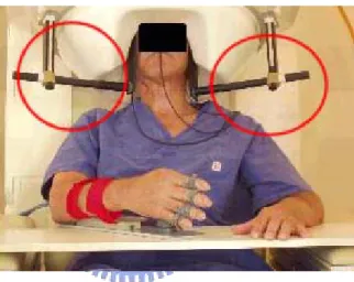
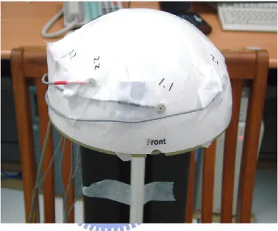
To MEG studies, head motion during MEG recordings acquisition is still a major prob-lem. To avoid this problem, one can just fix the subject’s head. However, this may cause many other problems. Keeping subject’s head fixed during MEG experiments may cause huge fatigue to the subject and this will disturb the quality of recordings. In Fig 1.8, a stroke patient’s head is fix during the experiment. This treatment is not only without humanity but also cause lots of fatigue. Furthermore, to many people, like Parkinson’s patients or to children, it is difficult for them to keep heads fixed. For these reasons, many algorithms are proposed to solve this problem.

Figure 1.8: This figure shows the stroke patient’s head is fix by the special device during experiments.

The easiest way is to discard the recordings with head motion. But this leads to longer time for experiments, may cause many other artifacts. Another approach is to correct head motion by incorporating the effect of the head motion into the magnetic field forward cal-culations [24, 25]. This may cause another problem of information loss.

Usually, the resolution of the solution to the MEG inverse problem can be improved by increasing the number of MEG sensors. The sensor number can only increase to some limited number. But this phenomenon is different to beamformer. To the problem about the sensor number needed [26, 27], we can understand that the sensor number of beamformer can be significantly large. The detailed description is stated in Chapter 4.

1.2

Thesis Scope

In this thesis, we have three major topics about how to reach the goal of source imaging with MEG modality. In the following, we briefly describe the topics in this thesis.

I. Statistical Evaluation of the Amount of Recordings

We take paired t-test as statistical hypothesis test to display the discrimination between the selected active and control states. By showing the p-value, we can find out some concepts about the amount of recordings.

II. Beamformer-based ICA

Our motivation is to combine MCB and ICA to get higher accuracy while keep-ing the information. By the concept of virtual sensors, we consider the filtered signal form the MCB spatial filter as the output from the virtual sensor at each voxel of interest and take them as the ICA input signal. In our thesis, we find out some ad-vantages for combining these two models and demonstrate it in the later sections.

III. Head Motion Correction

With a simple linear model applying to MCB, we can correct the problem caused from head motion easily and improve the accuracy of source localization by concep-tually increasing the sensor number. We will demonstrate the effect of this linear model in the later sections.

In this work, we implemented the proposed methods in C/C++ language on Win32 plat-form. The simulation of MEG recordings is conducted to validate the proposed algorithm. We also apply our methods to the recordings from real finger lifting, phamtom data and gender discrimination experiments.

1.3

Thesis Organization

At the later chapters, we will describe our methods in detail. First, we will depict how to find out the concept of the amount of MEG recordings by a statistical hypothesis test.

Then, we describe why and how to combine MCB and ICA for source localization. And we give a detail description of the problem about how to correct the head motion during MEG experiments. Finally, the discussion and a short conclusion for the thesis is given at the last chapter.

2.1

Statistical Evaluation of the Amount of Recordings

When conducting the event-related MEG experiment, we usually repeat the experiment many times and retrieve tens or hundreds of recordings to go on synchronized-averaging or single-trial analysis. If the amount of recordings is enough, we can get the more accurate solution to the inverse problem. But how to understand whether the amount of recordings is ”enough” is still an issue. There is still no criteria for the experimentalist to follow. Therefore, the number of recordings is usually manually determined by the experimentalist. Besides, there are many variations during experiments, including the condition of the subject, the various recordings between different subjects, different experimental paradigms, and interferences from the environment. As existing such many variations, it is difficult for the experimentalist to understand whether the amount of recordings is enough. We use statistical hypothesis test to reveal the discrimination between the selected active and con-trol states that the experimentalist can have some reference indicators about the amount of recordings.

2.1.1

Statistical Hypothesis Test

One may be faced with the problem of making a definite decision with respect to an uncertain hypothesis which is known only through its observable consequences. The hy-pothesis can be divide into two categories, research hyhy-pothesis and statistical hyhy-pothesis. Research hypothesis is also called scientific hypothesis that the scientists raise their ratio-nal hypothesis to their problems, according to theorems or documentations. The research hypothesis is represented by a statement.

When we express the research hypothesis with statistical terms or symbols, it becomes the statistical hypothesis. The statistical hypothesis includes null hypothesis and alternative hypothesis. We call a false hypothesis as null hypothesis and the alternative hypothesis is the opposite.

The statistical hypothesis must be stated in statistical terms and is able to calculate the probability of possible samples assuming the hypothesis is correct. Applying the statis-tical hypothesis, we often decide a null hypothesis which is opposite to our expectation.

Then test the abnormality with this null hypothesis by some statistical methods and decide whether this null hypothesis is hold. If this null hypothesis is rejected, our expectation is proved; otherwise, rejected. Therefore, how to state the null hypothesis is very important.

However, no matter rejection or acceptance of the null hypothesis, false decision still exists. If the null hypothesis is true, we still decide to accept it from the result of statistical test, and this is called Type I error. Type II error is just the opposite. The probability of type I error is often denoted as α and is called level of significance. The probability of type II error is often denoted as β. We often set the value of α as 0.05 or 0.01. In real world, Type I error is more serious than Type II error. As a result, we pay more attention to α than β.

Following the concept and purpose of statistical hypothesis test, we want to transform our problem about the amount of recordings into hypothesis for evaluation.

2.1.2

Evaluation of the Amount of Recordings with Statistical

Hy-pothesis Test

Assuming that the control state and the active state of brain signal are both random pro-cesses. Furthermore, the baseline state is weakly stationary and ergodic. We take a period of pre-stimulus recordings as the baseline state and a period of post-stimulus recordings as the active state, and take advantage of some statistical hypothesis test to reveal whether there is a significant difference between these two states.

We can follow the below procedure to construct a correct and reliable hypothesis test [28].

1. From the defined problem, identify the parameter of interest.

2. State the null hypothesis, H0 and specify an appropriate alternative hypothesis, H1.

3. Specify an appropriate test statistic.

4. Choose a significance level α and state the rejection region for the statistic.

5. Compute any necessary sample quantities, substitute these into the equation for the test statistic, and compute that value.

6. Decide whether or not H0should be rejected and report that in the defined problem and

retrieve the results.

Applying our problem into the above procedure, we can get the below statements.

1. The parameter of interest is the difference in mean between two different states, µ_cand µ_a. For each MEG channel i, the mean µciis calculated by averaging the recordings

mi during the selected control period, t = tcs. . . tce. The mean µai is calculated by

averaging the recordings during the selected control period, t = tas. . . tae.

For each channel i,

µci = E{|mi(t)|}, t = tcs. . . tce (2.1)

µai = E{|mi(t)|}, t = tas. . . tae (2.2)

where

µ_c = {µc1, µc2, . . . , µcN} (2.3)

µ_a = {µa1, µa2, . . . , µaN} (2.4)

and N is the number of MEG sensors.

2. H0:µc = µa, H1:µc 6= µa

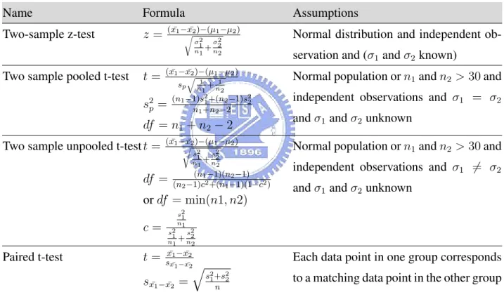
3. There are many kinds of statistical hypothesis tests (Table 2.1), we need to examine the data to be tested carefully to find the most appropriate hypothesis test. From 1., we want to test the difference in mean between two different states where the states are selected from each channel of recordings. We want to investigate whether there is a meaningful one-to-one correspondence between the data points in one state and those in the other. In the other words, we compare the data points of one channel in one state to those of the same channel in the other state by the statistical hypothesis test. Because of this special relationship, we take paired t-test as our hypothesis test.

4. α=0.05

6. From 5, we can get whether the null hypothesis is rejected or accepted to get the solution to our problem.

We apply the statistical hypothesis to the selected control and active states from the recordings and examine how the discrimination between two states variate as the number of recordings increase. From this variation, we can generate some reference indicators to help the experimentalist understand the amount of recordings.

Table 2.1: This Table lists some major statistical hypothesis tests, its assumption and formula.

Name Formula Assumptions

Two-sample z-test z = ( ¯x1− ¯x2)−(µ1−µ2) r σ2 1 n1+ σ2 2 n2

Normal distribution and independent ob-servation and (σ1and σ2 known)

Two sample pooled t-test t = ( ¯x1− ¯x2)−(µ1−µ2)

sp q 1 n1+ 1 n2 s2_p = (n1−1)s21+(n2−1)s22 n1+n2−2 df = n1+ n2− 2

Normal population or n1and n2 > 30 and

independent observations and σ1 = σ2

and σ1and σ2unknown

Two sample unpooled t-test t = ( ¯x1− ¯x2)−(µ1−µ2)

r s2₁ n1+ s2₂ n2 df = (n1−1)(n2−1) (n2−1)c2+(n1−1)(1−c2) or df = min(n1, n2) c = s2₁ n1 s2₁ n1+ s2₂ n2

Normal population or n1and n2 > 30 and

independent observations and σ1 6= σ2

and σ1and σ2unknown

Paired t-test t = x¯1− ¯x2 s_{x1− ¯}¯ _x2 sx¯1− ¯x2 = q s2 1+s22 n

Each data point in one group corresponds to a matching data point in the other group

2.2

Beamformer-based ICA

We propose a new method, Beamformer-based ICA, combining ICA with MCB to get higher accuracy source localization. Following the concept of virtual sensors from beam-former, we can combine MCB and ICA as Beamformer-based ICA. We consider filtered signals form the MCB spatial filter as the output from the virtual sensor at each voxel of in-terest and take them as the ICA input signal. We can obtain some advantages by combining MCB and ICA.

From section 1.1.2, we know that MCB is an efficient and accurate algorithm for source localization. However, the major problems in beamformer are the parameters needed to be well-selected, especially the regularization parameter α. α is a parameter to adjust the tradeoff between specificity and noise sensitivity. The inappropriate value of the regular-ization parameter can result in inaccurate spatial filter estimation. If we want a spatial filter with perfect spatial specificity, that α is 1 and the gain of the filter is 0 at every location expect the target one. This will result in that the norm of the spatial filter is too large and the leakage contributed from all other sources and sensor noise will make the spatial filter very unstable and sensitive to noises. If we take the utility of ICA into consideration, even with some inappropriate α, we can still use ICA to separate leakage from target source.

Although ICA is often used as the approach for noise separation [29, 30], it is a pow-erful method to separate signals into independent components. When we conduct signal analysis with ICA, we often observe temporal activations and the contribution to MEG sensors as topographic mapping of each independent component, when the input data is MEG recordings. From Eq (1.2), the topographic mapping corresponds to the column of W−1. As a result, the resolution of topographic mapping is limited with the input data. If we want to apply ICA for source localization problem, we must raise the resolution to tomographic mapping instead of using only recordings with limited number of sensors. Recently a method for ICA component topographic mapping is proposed [31], which is called Electromagnetic Spatiotemporal Independent Component Analysis (EMICA). It de-composes the mixing matrix A into L and B where L is the contribution of the tessellation element on the cortex to sensors, the same as lead field and B specifies the contribution of the source component to the tessellation element on the cortex. Instead of optimizing

A, this algorithm optimizes B as ICA components to reach the purpose of topographic mapping. Because it reconstruct the contribution in the brain cortex, EMICA still gets the result of topographic mapping.

If we take sources filtered from MCB filter, because of the concept of virtual sensors, we can raise the dimension of ICA input signals and accomplish tomographic mapping.

However, there exist a problem that if we take too many filtered signals as the ICA input, it will interfere the optimization in ICA because of too many noises. Using this method, we can use only target source activities as ICA input for reliable and accurate ICA components. Therefore, we need a threshold to remove the unnecessary noises. We calculate a threshold to extract only target source activities by a simple nonparametric statistical approach [3]. This approach uses maximum statistics [32] to address the multiple comparison problem [33]. It first standardize the empirical distribution of the filtered control recordings and then calculate the maximum T value at each pixel location. Finally, an empirical probability distribution from the maximum T value at each pixel location is obtained. By this empirical probability distribution with some significance level α, the threshold to extract only target source activities is generated.

The critical issue about ICA is the component selection. This is very subjective. Fur-thermore, ICA is sensitive to noise thus tends to incorrect selection of components. ICA component selection depends on temporal activities and topographic distribution. We can-not separate sources outside the brain, in which we are uninterested, according to the tem-poral and topographic information. If we apply MCB first and then ICA, like the algorithm of Beamformer-based ICA, we are able to separate sources outside the brain by using brain region information obtained from MRI. Then applying ICA further can result in indepen-dent brain activities by reducing leakage activities in MCB procedure. That’s the rea-son about the order of applying Maximum Contrast Beamformer (MCB) and Independent Component Analysis (ICA) in the algorithm of Beamformer-based ICA.

Therefore, by combining ICA with MCB, we use ICA to separate sources that fil-tered from MCB spatial filter to get more accurate solution to source localization. Using Beamformer-based ICA, we can ignore some inappropriate adjustment of the regulariza-tion parameter because the leakage is separated by ICA. Moreover, we can raise the ICA resolution of topography distribution in sensor space to the resolution of tomography

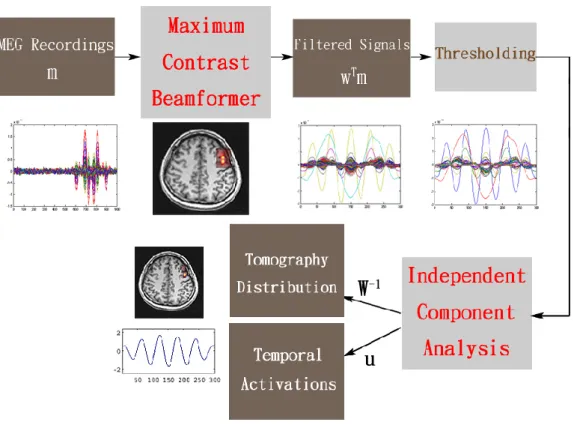
dis-tribution in source space using virtual sensor concept of beamformer. The overview of Beamformer-based ICA algorithm is in Figure 2.1.

2.3

Head Motion Correction

The head motion during MEG experiments will affect the accuracy of source localiza-tion. The simplest solution is that fixing the subject’s head. However, this may cause many other problems such as fatigue. And to many people, like Parkinson’s patients or to chil-dren, it is difficult for them to keep heads fixed. For the above reasons, many algorithm proposed to solve this problem.

The easiest way is to discard the recordings with head motion. But this leads to longer time for experiments and may cause many other artifacts. Another approach is to correct head motion by incorporating the effect of the head motion into the magnetic field forward calculations [24, 25]. This may cause another problem of information loss.

Usually, the resolution of the solution to the MEG inverse problem can be improved by increasing the number of MEG sensors. The sensor number can only increase to some limited number. But this phenomenon is different to beamformer. To the problem about the sensor number needed [26, 27], we can understand that the sensor number of beamformer can be significantly large. The detail description is stated in Chapter 4.

A newly-proposed novel method can improve the localization accuracy by conceptually increasing sensor numbers, instead of using motion correction [34]. By combining record-ings of different head poses, this algorithm can not only reduce the error induced from head motion but simultaneously improve the accuracy of source localization by conceptually in-creasing sensor numbers; i.e., super resolution. We describe this algorithm in the below sections.

2.3.1

Stabilized Linear Model

Starting from the same simplified form of MEG recordings, we assume that there are E epochs measured in an MEG study and there are N data samples collected for each epoch. Let mjbe the SxN matrix that denotes the epoch j of recordings and S is the MEG sensor

number, then

where Lj is the lead field matrix and s represents the dipole moment at each dipole

loca-tion. If there exists head motion during the period of recordings acquisition, Lj and s will

not remain the same for each epoch. Consequently, that directly averaging all epochs of recordings is incorrect and that may blurs the data and leads to a location bias.

In [34], a proposed method, Stabilized Linear Model (SLIM), can solve the problem of head motion. By continuously tracking the head pose, we can get the relationship of magnetic MEG sensors to the head with different poses and this relationship can be mod-eled as the forward problem which is necessary for the inverse problem [21]. Using SLIM, we can ransform the head motion during recordings acquisition into the increase of MEG sensor number. And by this concept, we can consider the dipole moment remains the same and ignore the subindex j. We can see this concept in Figure 2.2. Then, we can virtually have multiple sets of sensors measuring the MEG signals, mj, j = 1, ..., E, generated

from dipoles with moment s. The stabilized linear model is then obtained by combining the forward model for each epoch

       m1 m2 .. . mE        =        L1 L2 .. . LE        qs +        n1 n2 .. . nE        (2.6)

Using SLIM, we can improve the accuracy of source localization by conceptually in-creasing the sensor number. Even the recordings with head motion, by combining multiple set of recordings with different head poses, we can transform the localization bias induced by head motion into the improvement of the accuracy of source localization.

2.3.2

Solutions to Inverse Problem with Maximum Contrast

Beam-former

Because the resolution of the solution to the MEG inverse problem can be improved by increasing the number of MEG sensors, we apply the stabilized linear model into MCB to get higher accuracy of source localization.

Figure 2.2: This graph shows the concept of the algorithm of Stabilized Linear Model. If two epochs of MEG recordings with head motion are measured, we can represent the recordings as (a). If we transform the head motion into the increase of the MEG sensor number, by aligning the head in gray and in black in (a), we get (b). [34]

we can get mj = Ljqs + nj = ljs + nj j = 1, . . . , E (2.7) Eq (2.6) becomes        m1 m2 .. . mE        =        L1 L2 .. . LE        qs +        n1 n2 .. . nE        (2.8) =        l1 l2 .. . lE        s +        n1 n2 .. . nE        (2.9) ˜ m = ˜ls + ˜n (2.10)

where ˜m, ˜l and ˜n are all the combination from multiple sets of epochs with different head poses.

With Eq (2.7), the Beamformer spatial filter becomes

˜ wθ = ( ˜C + αI)−1˜lθ ˜lt θ( ˜C + αI)−1˜lθ (2.11)

where ˜C = cov{ ˜m(t)}.

With this linear model, we can virtually increase the sensor number of MCB model and get higher source localization accuracy, which can be called as ”super resolution”. Simultaneously, it can solve the problem induced from head motion.

3.1

Material

We used three kinds of data to verify the proposed methods depicted in Chapter 2, including simulation, phantom and the real measurement from the experiment of gender discrimination. For each proposed method, we select the appropriate data for validation. We will describe some information of these data in the below statements.

I. MEG Device

A whole head MEG system at the Taipei Veterans General Hospital (Neuromag Vectorview 306 , Neuromag Ltd., Helsinki, Finland) is used for recording of the minute magnetic field generated by electrical activity within the living human brain. The MEG system is placed in a magnetically shielded room and has capability of 306 channels simultaneous recording at 102 distinct sites, 24 bits analog to digital con-version, and up-to-8 kHz sampling rate which is sufficient to probe the fast dynamic changes inside human brains.

II. Anatomical Data

The Magnetic Resonance Imaging (MRI) images were from the 1.5T GE scanner at the Taipei Veterans General Hospital with TR = 8.672 ms, TE=1.86 ms, FOV = 26x26x10cm3, matrix size = 256x256, slices = 124, voxel size = 1.02x1.02x1.5mm3. III. Simulations

We simulate the MEG recordings by the forward model adding some noises with a dipole or dipoles given in advance. There are two kind of noises, background sources and sensor noises. We simulate background sources as random dipoles with zero-mean Gaussian strength and uniformly distributed in the putative sphere of head model. The variances of sensor noises are estimated from the empty room recordings of the MEG system. We also use 1 kHz sampling rate as sampling frequency of the simulated recordings. Before data analysis, we do preprocessing depicted in Section 3.2.

We use MEG phantom (Neuromag Ltd., Finland) to validate the localization ac-curacy of the proposed methods. Eight fixed current dipoles located on two orthogo-nal planes were activated sequentially to generate magnetic recordings. The strength of each dipole was set to be 100 nAm. For each dipoles, there are four combination of 20 trials from total 80 trials.We processed the phantom signals with bandpass filter and baseline correction. The device and configuration of MEG phantom are shown in Figure 3.1.

Figure 3.1: The device of MEG phantom. We can activate the dipole at the location of interest and retrieve the recordings of phantom data.

V. Experiment Paradigm of Gender Discrimination

Twenty normal subjects and twelve bipolar disorder patients participate this ex-periment. Face images are grayscale photographs of faces, depicting neutral, angry, happy and sad (Table 3.1). 306 channels were recorded during passive observation of face images in a electrically shielded MEG room. The task is to specify the gender of the presented faces that prevents the subject’s explicit recognition or categorization of the emotion expressed. Subjects are instructed to lift the right or left index finger while recognizing the presented face image as female or male. For each condition,

Figure 3.2: The dipole of phantom is generated by a triangular conductor with two radial lines connected by a tangential line. The location of each dipole is shown in this figure.

about 288 trials, 20 minutes are retrieved. The whole experiment paradigm is shown in Figure 3.3. We take the recordings of one normal subject for analysis. We also measure the finger lifting recordings while the subject is discriminating the gender of the presented faces. Both two kinds of data are included for the validation of our algorithms.

Figure 3.3: The experiment paradigm of gender discrimination. The task was to specify the gender of the presented faces. Subjects were instructed to lift the right or left index finger while recognizing the presented face image as female or male

Table 3.1: The stimuli were grayscale photographs of faces, depicting neutral, angry, happy and sad. Every kind of stimuli can also separate into male and female. The number of female stimuli is larger than the number of male stimuli.

state stimuli neutral male female angry male female happy male female sad male female

3.2

Data Preprocessing

The brain signal is comparatively small than the environmental noises. For signal-to-noise ratio (SNR) enhancement, preprocessing for the recordings is necessary before the further processing [35]. Generally, because the brain signal is usually modeled by ran-dom signals, we repeat the experiment several times to obtain sufficient amount of record-ings. The preprocessing steps we use for MEG recordings are as below statements. First, while conducting experiment, artifacts, body action and eye blinking can induce signifi-cant noises, compared to the real measurement. Hence, we can reduce artifact noise by finding out the abnormal scale of electric ocular graph (EOG) channels. Second, signal space projection (SSP) is often exploited to eliminate the unbalanced noise effect on dif-ferent sensors [36]. SSP is accomplished by calculating individual basis vectors for each term of the functional expansion to create a signal basis covering all measurable signal vectors. By this method, we can transform the interesting signals to virtual sensor config-urations [37]. Third, there are some unavoidable external artifacts, heartbeat, breath and power line noises. The artifact of heartbeat and breath is about one time per second (1 Hz), and power line is 60 Hz and its harmonic. Therefore, we use bandpass filter to ex-clude these artifacts. Moreover, the recordings on each sensors may drift along with time because of the device, so we need to conduct baseline correction. To take mean or peak recordings into analysis, any noise in the baseline will add noise to the input recordings. We conduct the baseline correction by subtracting a baseline from the recordings. The baseline is usually estimated by the mean of the recordings in the control state period, at which it assumes the recordings are unaffected by the stimulus. Finally, if the activation of interest is time- and phase-locked, according to the central limit theorem, we can eliminate the variance of the recordings contributed by the random noises, in proportion to the square root of trial numbers. We can align each trial of recordings by the onset time and average them synchronously. The all preprocessing steps are shown in Figure 3.4.

Figure 3.4: This graph shows the all preprocessing steps for MEG recordings. For SNR enhancement, preprocessing for the recordings is necessary before the further processing. First removing artifacts by finding out the abnormal scale of EOG channels. Then elimi-nating the unbalanced noise effect on different sensors by applying SSP. The next step is applying bandpass filter to remove the other artifacts like heartbeat and breath and some environmental noises like power line noises. The next step is to conduct the baseline cor-rection to eliminate the drift of recordings. After the whole process of preprocessing, we can go on for further analysis with enhanced SNR of recordings.

3.3

Statistical Evaluation of the Amount of Recordings

We use statistical analysis described in Chapter 2 to find a reference indicator to show the concept about the amount of recordings. We take the recordings of the left index finger lifting for statistical analysis. After preprocessing mentioned in Section 3.2, we select -350 ms to -200 ms as the control state and 0 ms to 150 ms as the active state. Then we apply paired t-test to the selected control and active states. We test two kinds of the control and active states. The one is after synchronously averaging from every trial of the raw recordings and the other is only the combination of every trial of the raw recordings. After applying paired t-test, we display the p-value under the significance level of 0.05 with increasing number of trials.

We find that the number of trials actually affects the p-value generated fro, applying average recordings of control and active states to paired t-test. The same effect also appears in raw recordings. The results are shown in Figure 3.5 and Figure 3.6. We sort the MEG sensors by their p-values and represents the corresponding p-value of each MEG sensor at the vertical axis. From this figure, we can find out that for both situations when the number of trials increase, the p-value becomes smaller, which also means more significant. Because of this phenomenon, we can set a evaluation criterion that when the number of sensors that reaches some significant level is as large as we expect, the amount of recordings is statistically sufficient.

Figure 3.5: Synchronously averaging recordings with increasing number of trials, for a period of 30 trials. Selecting the control and active states, and then applying the two states to paired t-test. From this figure, we can also find out that the p-value becomes smaller while the number of trials increase.

Figure 3.6: Selecting the control and active states from the raw recordings, without syn-chronously averaging. Then we apply the two states to paired t-test. From this figure, we can find out that the p-value becomes smaller while the number of trials increase.

3.4

Beamformer-based ICA

Following the concept of virtual sensors from beamformer, we can combine Maximum Contrast Beamformer (MCB) and Independent Component Analysis (ICA) as Beamformer-based ICA. We consider filtered signals form the MCB spatial filter as the output from the virtual sensor at each voxel of interest and take them as the ICA input signal. By com-bining ICA with MCB, we can use ICA to separate sources that filtered from MCB spatial filter to get more accurate solution. Using Beamformer-based ICA, we can ignore some inappropriate adjustment of the regularization parameter. Moreover, we can raise the reso-lution of ICA input data using Beamformer-based ICA to reach the purpose of topographic mapping.

When conducting experiments for Beamformer-based ICA evaluation, we take the cor-relation between sources into consideration. While there exists an implicit assumption in beamformer techniques that the time courses of the source activities should be orthogonal to each other; in the other word, all source activities should be completely uncorrelated [38]. We test Beamformer-based ICA for the utility of correlated sources. The experiment results are shown in the following statements.

We conduct the simulation data to validate Beamformer-based ICA. The strength of the two sources is both 30 nAm. Frequencies of the temporal profiles for the two sources are w0₁ and w₂0, where w0₁ is composed of w1 and w2, related to a coefficient ξ. We can adjust

the correlation between two sources with specified values of ξ. In this simulation data, we set w1 and w2 as 7 Hz and 17 Hz sinusoid signal.

w0₁ = (1 − ξ)w1+ ξw2

w0₂ = w2

We added background sources with 3000 random dipoles with the standard deviation of 10 nAm. The variances of sensor noises are estimated from the empty room recordings of the MEG system. Taking -500 ms to 0 ms as the control state and 0 ms to 500 ms as the active state, we calculate the MCB spatial filter. Under some specified regularization parameters, we take the filtered signals from MCB spatial filter as the ICA input. The α-significance level is set as 0.05 to extract only target source activities because too many filtered signals