行政院國家科學委員會專題研究計畫 期末報告
以實質選擇權解構待更新不動產價值之研究
計 畫 類 別 : 個別型 計 畫 編 號 : NSC 101-2410-H-004-204- 執 行 期 間 : 101 年 08 月 01 日至 102 年 07 月 31 日 執 行 單 位 : 國立政治大學地政學系 計 畫 主 持 人 : 陳奉瑤 計畫參與人員: 碩士班研究生-兼任助理人員:杜宇璇 大專生-兼任助理人員:吳孟璇 報 告 附 件 : 出席國際會議研究心得報告及發表論文 公 開 資 訊 : 本計畫涉及專利或其他智慧財產權,1 年後可公開查詢中 華 民 國 102 年 10 月 31 日
中 文 摘 要 : 近來,不動產市場因國際金融風暴、降低遺產與贈與稅、課 徵奢侈稅、推動都市更新等影響,致使不動產價格波動甚 大;而在租金變動不大但交易價格屢創新高情形下,更引起 一般購屋者甚至不動產估價師對不動產交易價格的內涵產生 疑惑。此外,近年越來越多文獻提出不動產價格隨屋齡增加 而價值反轉的探討,因而引發本計畫以實質選擇權的觀點, 解構不動產交易價格之動機。 本專題以使用價值與再開發實質選擇權價值建構不動產價值 模型,而以開發實質選擇權受時間與使用強度交互影響之觀 點,進行理論模型之推論;其後,於不動產典型特徵價格模 型的基礎下,運用半對數迴歸模型與分量迴歸進行實證,研 究成果顯示再開發選擇權普遍存在於老舊住宅,當老舊房屋 本身價值不同或所在區域不同,均會影響再開發選擇權價值 與標的價值之關係。老舊房屋價值直逼新成屋的現象,事實 上是土地之再開發選擇權價值所致,而且建物越舊、其再開 發價值越高,此與建物越舊價值越低之認知是不同之觀念, 必須匡正社會大眾正確的不動產價格認知。 中文關鍵詞: 再開發價值、實質選擇權、折舊
英 文 摘 要 : Recent years, real estate market is highly volatile due to the Financial Tsunami, Estate and Gift tax reduction, Luxury taxation, and urban renewal promotion. Buyers, or even real estate appraisers, are often confused in what price to take, especially when price increased continuously but when rent remained stable. Base on the increasing literatures proposing that real property value first decreases but then increase within its residual economic. It initiates the motivation to restructure the real estate price from real option theory. The
redevelopment option value is added in standard hedonic model and considered by the interaction term of age and intensity. Then semi-log multi-regression is adapted to process comparative analysis between various intensity and prosperity. The results show it is helpful to understand the factors forming the real estate knockdown price, increasing the cognition of social populace on the real estate bargain price, and rectifying the property price order.
行政院國家科學委員會補助專題研究計畫
□期中進度報告
■期末報告
以實質選擇權解構待更新不動產價值之研究
計畫類別:■個別型計畫 □整合型計畫
計畫編號:NSC101-2410-H-004-204-
執行期間:101 年 8 月 1 日至 102 年 7 月 31 日
執行機構及系所:國立政治大學地政學系
計畫主持人:陳奉瑤
共同主持人:
計畫參與人員:杜宇璇、吳孟璇
本計畫除繳交成果報告外,另含下列出國報告,共 1 份:
□移地研究心得報告
■出席國際學術會議心得報告
□國際合作研究計畫國外研究報告
處理方式:除列管計畫及下列情形者外,得立即公開查詢
□涉及專利或其他智慧財產權,■一年□二年後可公開查詢
中 華 民 國 102 年 10 月 30 日
I
摘要
近來,不動產市場因國際金融風暴、降低遺產與贈與稅、課徵奢侈稅、推 動都市更新等影響,致使不動產價格波動甚大;而在租金變動不大但交易價格 屢創新高情形下,更引起一般購屋者甚至不動產估價師對不動產交易價格的內 涵產生疑惑。此外,近年越來越多文獻提出不動產價格隨屋齡增加而價值反轉 的探討,因而引發本計畫以實質選擇權的觀點,解構不動產交易價格之動機。 本專題以使用價值與再開發實質選擇權價值建構不動產價值模型,而以開 發實質選擇權受時間與使用強度交互影響之觀點,進行理論模型之推論;其後, 於不動產典型特徵價格模型的基礎下,運用半對數迴歸模型與分量迴歸進行實 證,研究成果顯示再開發選擇權普遍存在於老舊住宅,當老舊房屋本身價值不 同或所在區域不同,均會影響再開發選擇權價值與標的價值之關係。老舊房屋 價值直逼新成屋的現象,事實上是土地之再開發選擇權價值所致,而且建物越 舊、其再開發價值越高,此與建物越舊價值越低之認知是不同之觀念,必須匡 正社會大眾正確的不動產價格認知。 關鍵詞:再開發價值、實質選擇權、折舊II
Abstract
Recent years, real estate market is highly volatile due to the Financial Tsunami, Estate and Gift tax reduction, Luxury taxation, and urban renewal promotion. Buyers, or even real estate appraisers, are often confused in what price to take, especially when price increased continuously but when rent remained stable. Base on the increasing literatures proposing that real property value first decreases but then increase within its residual economic. It initiates the motivation to restructure the real estate price from real option theory. The redevelopment option value is added in standard hedonic model and considered by the interaction term of age and intensity. Then semi-log multi-regression is adapted to process comparative analysis between various intensity and prosperity. The results show it is helpful to understand the factors forming the real estate knockdown price, increasing the cognition of social populace on the real estate bargain price, and rectifying the property price order. Keywords:redevelopment value, real option, depreciation
3
以實質選擇權解構待更新不動產價值之研究
一、
前言
近年來,受都市更新熱潮以及「台北市四、五層公寓舊屋更新專案」影響, 台北市舊公寓價格屢創新高,甚且高於大樓單價1。2009 年 10 月國有財產局標 售忠孝東路二段四層樓公寓,每建坪單價高達104 萬元;2011 年 11 月民事執行 處執行華山一期都市更新範圍內一37 年舊公寓的拍賣,以每建坪單價 115 萬拍 出,連連創下台北市公寓的天價,一般住宅也出現舊屋每坪價格接近當地新屋 或預售屋價格的情形。台北市公寓的交易價格屢創新高,但是房屋租金卻未見 明顯變動。於租金不見調漲但價格卻日益高昇下,社會大眾對不動產價格不僅 感到迷惘,甚至有追高助跌、盲目投資的疑慮。 不動產價值依 Rosen(1974)的特徵價格理論,係為資產各項特徵與其隱含 市場價值乘積之和;惟基於資本理論的複雜性,Rosen(1974:37)特別假設二手市 場不存在,排除資產於二手市場再出售的可能,然而真實之不動產市場,卻存 在著一次次的交易與再開發利用。國內近來不動產價格屢創新高、老舊公寓之 售價直逼新成屋價格的現象,似乎意味著:突破 Rosen 特徵價格理論二手市場 不存在假設,以各項特徵價格所形成之使用價值,與市場交易價格的關連性似 乎有所動搖。 老舊房屋以使用的角度而言,房屋老舊、規劃相對不合時宜、各項設施功 能不完備,以前述特徵價格模型之組成,其推估價格應相對較低;但近來的實 證研究 (Malpezzi, Ozanne and Thibodeau,1987; Goodman and Thibodeau,1995; Smith,2004; Wilhelmsson,2008, 梁仁旭、陳奉瑤, 2011) 指出,隨著屋齡的提高,不動產價格出現反轉現象,呈現微笑U 曲線。顯然,以不動產各項特徵為主要
組成之特徵價格模型,用以衡量並解釋現今台灣不動產市場,可能有重要因素 存在於誤差項中而未被考量之情形。
房屋越舊、價格越高的現象,Lee, Chung and Kim(2005)認為隨著建物屋齡 的增加,不動產更新的可能性提高;如果再開發存在經濟利益,則更新預期淨 利之資本化將對不動產價格產生正面影響。其後,Clapp and Salavei(2010)、Clapp, Salavei and Wong(2012)亦基於相似的觀點,而於理論上建立不動產價值包含使 用價值與再開發選擇權價值的模型,作為實證分析的基礎。前述文獻中,Clapp and Salavei(2010)、Clapp, Salavei and Wong(2012)以土地現況使用強度為再開發 價值的替代變數,實證結果顯示現況使用強度越低、越容易再開發,而使再開 發擇權價值與不動產價值越高。 本專題透過加入實質選擇權替代變數理論模型之推論,論述老舊公寓售價 1 98 年大安區公寓平均拍定價為每坪 47.02 萬,大樓為每坪 43.22 萬,較公寓少 3.8 萬。詳參 http://money.udn.com/house/storypage.jsp?f_ART_ID=206269#ixzz1g2daXkIm
4 直逼新成屋價格的現象後,再以實證分析驗證並說明我國不動產價格的再開發 選擇權價值。綜合前述,本專題設定研究目的如下: 1. 依實質選擇權理論建構具再開發價值之不動產價值模型,並以為實證分析 基礎。 2. 實證估計再開發實質選擇權價值,釐清不動產交易價格之內涵。 3. 比較分析不同開發程度地區、不同交易價格層級之再開發實質選擇權價值 是否存在,及其對價值之影響程度。 4. 依據分析結果提供正確之不動產價格認知,以健全市場機制。
二、
文獻探討
Dixit and Pindyck(1994)主張當投資決策具有不可回復性、不確定性及投資 時間彈性等特性時,投資計畫具有選擇權價值。不動產投資開發決策於性質上 具有上述三項特性,因此,不動產應具選擇權之價值。而待更新老舊公寓不動 產,於都市更新前之交易價格直逼新成屋價格的現象,可以此選擇權價值加以 解釋。 有關不動產實質選擇權之研究,Titman(1985)首先以二期的二項式選擇權定 價模型,建立都市可建築空地價格模型,推論不確定性的增加將減緩開發建築 行為;Williams(1991)亦將實質選擇權理論應用於土地價格評估中,探討空地開 發與再開發最適時機與規模的選擇。而後,Quigg(1993)以美國 Washington 州 Seattle 地區已開發不動產真實交易價格,採特徵價格模型建立可開發不動產價 格彈性函數後,對已開發不動產的樣本以特徵模型估計空地的最適建築價格, 以估計使用價值上增加的實質選擇權價值,其研究發現都市住宅用地價格包含 1%至 11%的選擇權溢價。之後 Anthony and Roger(2004)以美國 Illinois 州 Champaign 地區空地與已開發不動產的資料,藉由特徵價格理論進行實證分析, 推估可開發住宅土地的價格中,選擇權時間價值約佔土地價值之 32%。陳奉瑤 (2003)以待更新土地為對象,經由模型推導而得實質選擇權存在價值中,並以模 擬方式模擬各變數變動對待更新土地價值的影響;梁仁旭(2007)則以實證結果指 出,我國的選擇權時間價值約佔空地價值之 11.96%,且越接近開發成熟階段比 值越低。上述相關文獻皆以可能開發之土地為對象進行實證研究,忽略了已開 發不動產亦可能存在選擇權價值的探討。 實質選擇權的探討,之後漸漸發展至可能拆除重建之不動產,Rosenthal and elsley(1994) 著 重 於 住 宅 拆 除 與 再 開 發 抉 擇 的 探 討 。 Brueckner and Rosenthal(2006)以及 Rosenthal(2008) 指出位於高地價地區的折舊後建物,較易 引發再開發。Dye and McMillen(2007)運用特徵迴歸,分析建物獲得可拆除允許 下之再開發時點的價值評估。Clapp and Salavei(2010)於 Connecticut 州
5
Greenwish 的實證以及 Clapp, Salavei and Wong(2012)於 Connecticut 州的實證研 究,均以附加於不動產使用價值上的再開發選擇權價值為對象;梁仁旭、陳奉 瑤(2009)於高雄市的實證研究亦以不動產為標的,探討隨時間變動的實質選 擇權價值變動情形。彭建文、馮靖博、丁玟甄(2011)藉由模型推導與模擬方式, 驗證待更新不動產選擇權價值之存在。其雖於價值模型中加入選擇權價值並加 以推導,但後續模擬分析時卻少了影響選擇權價值的重要變數--時間,少了時間 的變動,自然難以掌握隱含不確定性的選擇權價值。
前述文獻中,Clapp and Salavei(2010:364)只提及價格依幾何布朗寧運動變
動,就直接設定選擇權價值為 (q ) 、 0,並設定實證模型為使用價
值與再開發選擇權價值;另於實證模型中假設建築為高強度使用時,執行價格 會增加,而直接令現有使用強度的平方項係數為負,此等均未見於理論推演過 程中加以說明,較缺乏說服力。另依 Hulten and Wykoff(1981)、Cannaday and Sunderman(1986) 、 Malpezzi, Ozanne and Thibodeau(1987) 、 Goodman and Thibodeau(1997)、梁仁旭(2011)等之研究,不動產價值於耐用年限內隨屋齡 增加而先減後增,其呈現之逆折舊現象為再開發價值之結果;然而 Clapp and Salavei(2010)一文之實證中,使用價值包含了建物屋齡及屋齡的平方項,如此可 能將部分再開發選擇權價值納入使用價值中,造成再開發選擇權價值有低估之 嫌疑。
Clapp, Salavei and Wong(2012)基本上依循 Clapp and Salavei(2010)之作法, 將其擴展至全州各城鎮的比較研究,上述問題承續而相同存在。實質選擇權價 值早已被模型化,本專題期望承續 Lee, Chung and Kim (2005)與梁仁旭、陳奉 瑤(2009)之理論推導,將不動產價值由土地價值與建物價值之組成,修改為 使用價值與再開發選擇權價值,以再開發選擇權價值為依附於不動產使用價值 之非負附加價值為主張,進行理論推演。 此外,基於折現現金價值的最大化,投資者會考慮投資的時間點,亦即,不動 產價值會受到時間的影響,因而於價值上需考量選擇權價值。許多文獻以不同 的不確定性與總體不動產開發,探討並支持實質選擇權理論之間的交互作用, 例如 Sivitanidou and Sivitanides(2000)發現商用不動產的建築比率越低,不動產 需求的波動越大;淨獲利不確定性較高的地方,開發者越喜歡去開發(Wu and Cho, 2007)、單戶住宅的開發者傾向延遲開發(Mayer and Somerville, 2000)。 Cunningham(2007)更指出,不確定性提高一個標準差,將使開發機率降低 11%, 而空地價格上漲 1.6%,但若已離開可能開發的界限,價格的不確定性就不會影 響投資行為。此即意味著,若無再開發價值,則藉由實證模型估計附加於開發 或再開發選擇權的價值將接近於 0,將回歸 NPV 法則中的價值。無怪乎 Grenadier(2002)指出,競爭將使大部分、甚至全部的延遲選擇權價值消失。 相關文獻中多在證明實質選擇權的存在,並驗證各變數與實質選擇權的變動方 向,例如:Malpezzi, Ozanne and Thibodeau(1987) 、Lee, Chung and Kim(2005) 、
6
Clapp and Salavei(2010)、梁仁旭和陳奉瑤(2011)認為建物經過一段時間以後,隨 著屋齡的增加不動產價格會不減反增;Holland, Ott and Riddough(2000)認為以商 用不動產而言,建築比例與系統風險或全部的風險在短時間內會有負向關係; 陳奉瑤(2003)、彭建文、馮靖博、丁玟甄(2011)之模擬結果跟所有選擇權理論一 樣,價格波動與實質選擇權呈正向變動。
過去僅少數文獻以不動產資料庫進行實證分析,估計不動產再開發選擇權 價值。例如:Clapp and Salavei(2010)以 Connecticut 州的 Greenwish,強調以該 城市空間特徵詳細資訊為基礎,進行附加於不動產使用價值上的再開發選擇權 價值研究;Clapp, Salavei and Wong(2012) 建構可界定個別財產高選擇權價值 的實證方法,選擇某一屋齡以上的不動產,以各城鎮為單位檢測實質選擇權的 價值,並用以檢視選擇權價值與波幅及其他預期相關變數間之關係,二者認為 不動產交易價格中可能隱藏再開發之實質選擇權價值,低密度區空地較多,將 會降低其他資產之選擇權價值;低價區之實質選擇權價值將較低;低價格波動 地區,實質選擇權價值亦較低;梁仁旭和陳奉瑤(2011)以台北市之不動產價格資 料與租金資料,分析不動產價值隨時間經過而發生之屋齡效應變化情形加以分 析,驗證不動產屋齡效應的逆折舊現象源於土地而非建物。 至於再開發選擇權
價值的衡量,Clapp and Salavei(2010)藉由建築物評估價值與土地評估價值之 比值,以非線性型式納入含再開發選擇權的標準特徵模型,亦即以建物價值與 土地價值比,作為衡量再開發實質選擇權的替代變數加以量測;Clapp, Salavei and Wong(2012)認為以屋齡與基地大小為變數,可用以捕捉再開發選擇權價值; 梁仁旭和陳奉瑤(2011)以台北市之不動產價格資料與租金資料,藉由租金資料推 估使用價值,並將不動產交易價格與使用價值間的差距,視為再開發選擇權價 值。惟梁仁旭與陳奉瑤(2011)是否可將兩者間的差距直接視為再開發選擇權價值, 仍有待斟酌。Bourassa et al.(2011)指出,土地價值和建物價值不會以相同的比例 變動,運用土地槓桿的程度解釋不動產價值的變化益形重要。如前所述,實質 選擇權理論主張土地價值會隨建物價值的下降而升高;且不動產估價理論主張 不動產再開發價值減去開發成本和現有使用價值若大於 0,表示經濟耐用年限 已至,不再為最有效使用。因此,如能參考土地槓桿等相關文獻提出之使用強 度作為衡量基礎,或可利用現況使用密度是否接近最有效使用;或現況使用價 值與最有效使用價值間之比值關係,作為實質選擇權價值之替代變數,進行實 證分析,或許更能真實掌握再開發選擇權價值之影響。是以,引發本研究加入 使用強度深入考量再開發選擇權價值之動機。 基於此,本專題將依選擇權價值理論,建立再開發前、後兩階段價值組合 之使用價值與再開發價值的基礎上,建構並推導不動產價值模型,論述老舊公 寓售價直逼新成屋價格的現象後,再以使用強度等實質選擇權之替代變數實證 分析驗證並說明我國不動產價格的再開發選擇權價值。
7
三、
研究方法
本專題將先建立含有時間價值的不動產價值模型,該模型中將包含使用價 值與選擇權價值兩項,前者為一般所謂的不動產價值,亦即依典型特徵價格模 型而得之不動產價值;後者為隨著時間變動而不同的再開發價值,即為再開發 選擇權價值。而後將藉由特徵價格模型的組成,以迴歸分析階段式的一一驗證。由於Clapp and Salavei(2010), Clapp, Salavei and Wong(2012)等指出,再開 發之實質選擇權價值會因開發密度與價格高低、價格波動等差異而有所不同, 故本專題分別建立典型不動產價值模型、以分量迴歸方法建立再開發選擇權價 格模型。以下分別說明驗證所需建立之理論模型與實證分析方式: (一)、理論模型 投資時,如將選擇權價值納入決策考量,假設不動產開發後使用收益R2(t) 依循幾何布朗寧運動,亦即: dz R dt R dR2 2 2 (1) 其中dR 為不動產再開發以後收益之變動,μ 為開發後收益之預期成長率; σ 為開發後預期收益波動之標準差,代表外生的不確定性風險程度;dt 為時間 t 之變動;z 為與時間有關,且依循標準韋那過程變動之變數;dz 為 z 之變動、 dz=
t dt,dz~(0,dt);μ 及2 隨時間呈固定變動。R2dt為開發後收益預期變 動之部分;而R2dz為開發後收益變動中非屬預期之部分,呈常態分配。 不確定下,可將式(2)改寫為:
rD D t ) r ( 1 2 1 D r [R (t) R (t)]e dt C e ) t ( R E ] V [ E Max
E R1(t)r WR (2) 此時開發決策在使W
R 極大化,亦即:
D rD t r D W R E R t R t e dt C e Max ( ) 1 2( ) ( )] [ ) ( (3)
R W 可視為在不同R(t)下,不動產再開發的選擇權價值,此價值依無 套利原則,可藉由依伊藤定理(It 's Lemma)導出其最適開發時機選擇權價值 的二階微分方程式: 0 W ) r ( W R W R 2 RR R 2 2 (4)8 選擇權價值除需滿足上列均衡條件外,價值本身亦需滿足下列之邊界條件
0 0 W (5)
R
R
t R
t
e dt c W r t
0 ) ( 1 2 * (6)
R r W R * (7) 是以,選擇權價值W(R),其一般解可設定為:
R A R W (8) 對W
R 求一階導數可得WR
R A
R1、求二階導數可得
R A( 1)R2 WRR ,代入式(4)中,則 0 ) ( ) 1 ( 2 1 2 2 2 AR r R A R R A R ,依此可得式(7)之特性方程式
1
(r ) 0 2 1 2 ,求解上式可得 其中, 2 2 2 2 2( ) 12 2 1 r 為負值,不符邊界條件,故取 2 2 2 2 2( ) 12 2 1 r ,且β>1;而 2 1 1 ( 1) 1 r ] C r ) ( R ) ( R [ A D D (9) 而不動產最適開發時機應選擇在:
)[R (D) r C] 1 ( D R 1 (10) 選擇權價值A R為R2(D)和R1(D)的函數,因此,後續將可藉由對R2和R1 間的差異,間接分析再開發之選擇權價值。 (二)、實證分析 透過前述模型,推導並描述再開發選擇權價值的存在。因此,本專題認為 若缺乏對選擇權價值的評估,利用特徵價格模型的估價結果將產生偏誤。為分 析不動產價格之再開發實質選擇權,將依循相關文獻實證分析所採之特徵價格 模型,建立迴歸式進行實證分析。有關實證分析之實證模型說明如下: 2 2 2 2 2( ) 12 2 1 r9 1.典型模型(含再開發實質選擇權替代變數)
特徵價格模型之雛型最早由Haas 於 1922 年提出,Court 於 1939 年正式賦 予特徵價格(Hedonic)一詞,而後由 Rosen(1974)確立特徵價格模型之理論基礎 (Sirmans, Macpherson & Zietz(2005);Wilhelmsson, 2008)。該模型假設不動產價 格為其各部份特徵價格之總合,藉由迴歸分析結果,可瞭解影響價值之特徵及 其影響強度,估計各項影響因素之影子價格、解釋價值的差異,並推估合理之 價格。
特徵價格模型之雛型最早由Haas 於 1922 年提出,Court 於 1939 年正式賦 予特徵價格(Hedonic)一詞,而後由 Rosen(1974)確立特徵價格模型之理論基礎 (Sirmans, Macpherson & Zietz(2005);Wilhelmsson, 2008)。該模型假設不動產價 格為其各部份特徵價格之總合,藉由迴歸分析結果,可瞭解影響價值之特徵及 其影響強度,估計各項影響因素之影子價格、解釋價值的差異,並推估合理之 價格。
本專題參考Follain and Malpezzi(1980),Smith(2004)、Fisher et al.(2005)、 Wilhelmsson(2008)等文獻,採半對數特徵模型為實證模型,模型如式(11): i n m k ki k m j ji jX β D ε β α ) i Ln(P
1 1 0 (11) 其中, 第i 個樣本土地價格的自然對數; 截距項; 第i 個樣本第 j 個連續性特徵屬性; 第i 個樣本第 k 個虛擬特徵屬性; 第j 個特徵之係數值; 第k 個特徵之係數值; 屋齡特徵之係數值,因應分析內容,包含屋齡或屋齡平方; 第i 個樣本之常態分配誤差項。 2.分量模型 由於彭建文、馮靖博、丁玟甄(2011)於部分地區(如萬華區)之實證結果; Clapp, Salavei and Wong(2012)於 Connecticut 州之部分城鎮的實證結果與預期不符(應具有更新選擇權價值但實證結果卻非如此)。本文推測前述研究未考量不 動產價格不同之標的,或標的所在區域不同時,隱含實質選擇權將有不同,導 致成效不顯著。 因此,本專題除了藉由價格簡訊資料庫獲得典型特徵價格模型資料外,選 擇尚有發展性及已成熟發展之地區進行研究。此外,透過分量迴歸分析,分別 以交易價格 25%、50%、75%,抽取交易樣本進行實證。其中,如式(12)所示, 以屋齡及屋齡平方變數作為再開發實質選擇權之替代變數,用以測試本專題依
10
11 其中, 第i 個樣本土地價格的自然對數; 截距項; 第i 個樣本第 j 個連續性特徵屬性; 第i 個樣本第 k 個虛擬特徵屬性; 第j 個特徵之係數值; 第k 個特徵之係數值; 屋齡特徵之係數值,因應分析內容,包含屋齡及屋齡平方; 第i 個樣本之屋齡特徵屬性; 第i 個樣本之常態分配誤差項。 3.研究資料說明 不動產交易價格資料主要取自內政部民國95 年至 101 年每季定期發佈之房 地產交易價格簡訊,為比較成熟發展地區與新興發展地區之再開發選擇權價值 是否不同,本專題透過三民區及左營區透天住宅交易資料建構實證模型。其中, 高雄火車站位於三民區,為高雄陸上主要交通樞紐之一,故三民區為已成熟發 展地區。至於左營區過去主要為海軍重要基地,自台鐵、高鐵、捷運左營站三 鐵共站完成後,成為高雄的轉運中心之一。此外,民國98 年世界運動會主場館 (現為國家體育場)及高雄市現代化綜合體育館(高雄巨蛋)均位於左營區, 使左營區成為高雄之新興發展地區。刪除因資料缺漏、有明顯錯誤之樣本後, 三民區共1931 筆透天住宅交易資料、左營區共 572 筆透天住宅交易資料。 基於再開發價值主要存在於土地而非建物,故實證模型之因變數為土地價 格;建物價格係透過建物標準單價表計算而得,土地價格則由不動產價格中分 離扣減。因樓層別效用比推算於操作上有所困難,致殘餘之土地價格仍隱含立 體利用價值,故於選擇自變數時,仍納入「建物面積」變數。 實證所需資料內容除實證所需之應變數交易價格外,尚有建造日期、土地 面積、建物面積、土地屬性等影響不動產價格因素,經處理後可為自變數資料。 此外,為提高模型解釋能力,將藉由地理資訊系統,依交易樣本之門牌位置結 合建物門牌查詢系統(或 XY 座標)產製各項公共設施距離之區位資料,以擴 充解釋變數。至於各變數性質、敘述統計說明如下:
12 表1 變數說明 變數名稱 變數 類別 預期 符號 說 明 拆分後土地價格 (因變數) 連續 以不動產交易價格扣除以成本法計算之建物價格後之 土地剩餘價值。 96 年 虛擬 + 1 代表樣本於 96 年交易、0 則否 97 年 虛擬 + 1 代表樣本於 97 年交易、0 則否 98 年 虛擬 + 1 代表樣本於 98 年交易、0 則否 99 年 虛擬 + 1 代表樣本於 99 年交易、0 則否 100 年 虛擬 + 1 代表樣本於 100 年交易、0 則否 101 年 虛擬 + 1 代表樣本於 101 年交易、0 則否 道路路寬 連續 + 建物面臨道路之寬度 宗地形狀 虛擬 + 1 代表樣本基地為方形、0 則為不規則形 土地移轉面積 連續 + 所位基地面積 建物移轉面積 連續 + 建物樓地板面積 屋齡 連續 - 建物建築完成日期至案例交易時所經歷之年數 與火車站反距 連續 + 樣本距火車站最短路徑距離與影響範圍之差額 與捷運站反距 連續 + 樣本距捷運站最短路徑距離與影響範圍之差額** 與購物中心反距 連續 +/- 樣本距購物中心最短路徑距離與影響範圍之差額** 資料來源:房地產交易價格簡訊、地理資訊系統計算結果 *:由於以成本法拆分建物價格與土地價格時,未能考量到樓層別效用比及交易價格與土地 面積間之關係非線性對價格造成的影響,故雖然以土地價格為因變數,仍將「建物面積」 變數納入模型中,且公寓樣本再將「交易樓層是否為一樓、四樓與頂樓」移轉納入模型 中。 **:本文以勘估標的為中心,半徑1500公尺以內公共設施之影響為範圍,因此以樣本點距該 公共設施最短路徑距離與1500公尺之差額為觀察值;而影響範圍外之樣本,其觀察值設 為0。例如:樣本距離學校300公尺,則其與學校反距為1200公尺;若距離學校1500公尺, 則其與學校反距為0公尺,不生影響。換言之,一般性公共設施迴歸係數之預期符號為正、 嫌惡設施為負。
13 表2 連續變數之敘述統計 區域 三民區 左營區 變數 最小值 最大值 平均數 標準差 最小值 最大值 平均數 標準差 土地總價(萬元) 75.34 4800.17 479.95 345.22 118.93 8128.63 853.23 654.99 土地單價(萬元/坪) 1.59 88.50 20.95 9.49 9.06 72.25 27.70 11.21 土地總價占房地總價比 63.00% 98.36% 87.71% 4.96% 62.85% 98.76% 87.31% 4.06% 道路路寬(m) 3.00 70.00 13.71 9.27 2.00 45.00 16.78 8.70 土地移轉面積(/m2) 21.00 467.00 73.15 29.75 23.00 1196.25 97.41 61.73 建物移轉面積(/m2) 36.00 854.00 151.66 82.04 21.00 939.4 215.38 117.76 屋齡(年) 0.08 54.92 28.28 11.25 0.00 46.92 13.61 13.46 與火車站距離(100 m) 0.50 43.65 23.26 10.78 4.14 39.00 23.93 8.26 與捷運站反距(100 m) 0.49 14.99 8.04 3.91 0.67 14.90 7.54 3.35 與購物中心反距(100 m) 1.15 14.91 9.32 3.57 1.08 14.97 10.16 3.73 資料來源:整理自房地產交易價格簡訊資料 表3 虛擬變數之敘述統計 變數名稱 變數內容 三民區 左營區 透天 透天 次數 % 次數 % 年度 95 年交易樣本 374 19.4 141 24.7 96 年交易樣本 364 18.9 142 24.8 97 年交易樣本 347 18.0 83 14.5 98 年交易樣本 308 16.0 100 17.5 99 年交易樣本 293 15.2 53 9.3 100 年交易樣本 172 8.9 32 5.6 101 年交易樣本 73 3.8 21 3.7 臨街關係 臨街地 690 35.7 330 57.7 路角地 17 0.9 6 1.0 裡地 1224 63.4 236 41.3 宗地形狀 方形 1832 94.9 486 85.0 不規則形 99 5.1 86 15.0 資料來源:整理自房地產交易價格簡訊資料
15
四、
實證結果
(一)、三民區 由一般之特徵價格模型觀察,再開發選擇權變數均為顯著,代表三民區之 透天住宅土地隱含在開發選擇權價值。而由圖 1 所示當屋齡越高,三民區透天 住宅之土地價值有先增後減之現象。進一步以不同價位交易標的觀察,本研究 以75%分量、50%分量、25%分量代表交易資料中之高交易總價標的、中交易總 價標的及低交易總價標的。由實證結果可知,不同分量之迴歸結果不盡相同。 其中,代表再開發價值之屋齡其屋齡平方變項,於低價資料中屋齡平方變 項不顯著;中價資料及高交易總價標中,屋齡及屋齡平方變項均為顯著。代表 在三民區,透天類型之不動產若為低交易總價之標的,隨時間增加,屋齡對土 地價格之關係為線性關係。而中高交易總價之標的,屋齡與土地價格呈非線性 關係。 若以圖形表示屋齡、屋齡平方變項與土地價格之關係2,如圖1 所示,高交 易總價之標的第35 年為土地價值最低點。亦即隨屋齡增加,土地價值有先增後 減之反轉現象,故高價交易標的具有再開發可行性;中交易總價之標的,雖屋 齡平方係數為正,惟其土地價值雖時間增加先增後減之情況不明顯,無土地再 開發之可行性;低總價地區屋齡平方係數不顯著,但屋齡係數顯著且係數為負, 代表隨時間增加,土地價值降低。 綜而言之,於三民區之透天住宅中,高交易總價之房屋,其再開發可行性 較高;而中、低交易總價之房屋則尚無再開發可行性。若探究原因,可能高價 之房屋本身就較具價值,而價值來源可能來自於周圍環境或標的房屋本身,故 市場預期該高價標的再開發後,亦能有較高之交易價格與獲利,故再開發價值 較中低交易總價之標的來得高。 2 土地價值比例=EXP(屋齡係數*屋齡+屋齡平方係數*屋齡平方)16 表 4 三民區實證結果 OLS 25%分量 50%分量 75%分量 96 年 -0.03381 ** -0.03537 *** -0.01012 -0.04114 *** 97 年 0.04519 *** 0.06068 *** 0.05604 ** 0.01002 *** 98 年 0.13976 *** 0.09684 *** 0.11707 *** 0.11447 *** 99 年 0.16747 *** 0.11635 *** 0.13979 *** 0.13388 *** 100 年 0.24249 *** 0.20004 *** 0.22152 *** 0.21745 *** 101 年 0.32792 *** 0.26588 *** 0.33809 *** 0.32107 *** 路寬 0.00547 *** -0.00041 0.00272 *** 0.00665 *** 臨街地 0.34210 *** 0.31343 *** 0.34433 *** 0.33188 *** 街角地 0.37080 *** 0.27792 *** 0.47470 *** 0.34025 *** 形狀 0.07006 *** 0.00192 0.04810 *** 0.03309 *** 土地面積 0.72947 *** 0.80804 *** 0.80801 *** 0.67931 *** 建物面積 0.34223 *** 0.22556 *** 0.24617 *** 0.38985 *** 屋齡 -0.01256 *** -0.00678 *** -0.01060 *** -0.01438 *** 屋齡平方 0.00017 *** -0.00004 0.00007 *** 0.00016 *** 距火車站反距 -0.00004 *** -0.00006 *** -0.00006 *** -0.00005 *** 距捷運站反距 0.00021 *** 0.00014 *** 0.00017 *** 0.00019 *** 距大型百貨反距 -0.00024 *** -0.00019 *** -0.00021 *** -0.00021 *** 截距項 10.35337 *** 10.73056 *** 10.63196 *** 10.66551 *** Pseudo-R2 0.861 0.661 0.686 0.682 註:1%顯著水準以***表示;5%顯著水準以**表示;10%顯著水準以*表示 圖 1 三民區透天住宅屋齡與土地價值關係圖 .00 20.00 40.00 60.00 80.00 100.00 120.00 0 3 6 9 12 15 18 21 24 27 30 33 36 39 42 45 48 51 54 現 值 比 例 屋齡 75% 50% 25% OLS
17 二、左營區 先就代表再開發價值之屋齡及屋齡平方變項觀察,左營區透天住宅之再開 發選擇權變數變動方向與三民區透天住宅類似。於一般之特徵價格模型結果觀 察,屋齡及屋齡平方項均為顯著,代表左營區透天住宅之土地價值隱含再開發 選擇權價值。 若以分量迴歸觀察不同價位之交易標的,於左營區低價標的中,屋齡平方 變項不顯著;中價標的及高價標的則屋齡及屋齡平方變項均為顯著。代表在左 營區之透天類型不動產若為低交易總價之標的,隨時間增加,屋齡對土地價格 之關係為線性關係。而中高交易總價之標的,屋齡與土地價格呈非線性關係。 若以圖形表示屋齡、屋齡平方變項與土地價格之關係,如圖 2 所示,中、 高交易總價之標的,隨屋齡增加,有土地價值先增後減之反轉現象,代表高價 值交易標的具有再開發可行性;低總價地區屋齡平方係數不顯著但屋齡係數顯 著且係數為負,代表隨時間增加,土地價值降低。此外,高交易總價之實證顯 示於第26 年為價格之最低點,中價地區則是第 32 年為價格最低點。 綜而言之,於左營區之透天住宅中,中、高交易總價之房屋,其再開發可行 性較高;且價值越高,再開發可行性出現之時點越早。至於左營區低交易總價 透天住宅則尚無再開發可行性。
18 表5 左營區實證結果 OLS 25%分量 50%分量 75%分量 96 年 0.02219 -0.01543 *** 0.02301 0.04726 97 年 0.27445 *** 0.28759 *** 0.25891 *** 0.23355 *** 98 年 0.28992 *** 0.30806 *** 0.28274 *** 0.24125 *** 99 年 0.34137 *** 0.36893 *** 0.33537 *** 0.28643 *** 100 年 0.37739 *** 0.31947 *** 0.40700 *** 0.39499 *** 101 年 0.38307 *** 0.41692 *** 0.37147 *** 0.35334 *** 路寬 0.00746 *** 0.00590 0.00659 *** 0.00716 *** 臨街地 0.18889 *** 0.20429 *** 0.19278 *** 0.15757 *** 街角地 0.30836 *** 0.27776 *** 0.25386 *** 0.29690 *** 形狀 -0.00096 0.03434 -0.01211 0.02854 土地面積 0.60058 *** 0.57494 *** 0.54673 *** 0.58809 *** 建物面積 0.44192 *** 0.39671 *** 0.48398 *** 0.52208 *** 屋齡 -0.02299 *** -0.01887 *** -0.02164 *** -0.01974 *** 屋齡平方 0.00037 *** 0.00017 0.00034 *** 0.00038 *** 距火車站反距 0.00004 *** 0.00004 *** 0.00005 *** 0.00005 *** 距捷運站反距 0.00016 *** 0.00019 *** 0.00018 *** 0.00016 *** 距大型百貨反距 -0.00001 -0.00004 -0.00002 -0.00005 截距項 10.30609 *** 10.53412 *** 10.32094 *** 10.01341 *** Pseudo-R2 0.908 0.725 0.725 0.721 註:1%顯著水準以***表示;5%顯著水準以**表示;10%顯著水準以*表示 圖2 左營區透天住宅屋齡與土地價值關係圖 .00 20.00 40.00 60.00 80.00 100.00 120.00 0 3 6 9 12 15 18 21 24 27 30 33 36 39 42 45 48 51 54 現 值 比 例 屋齡 75% 50% 25% OLS
19
五、
結論
本專題透過再開發選擇權理論模型的建立,驗證再開發選擇權的存在, 而後由三民區透天住宅資料、左營區透天住宅交易資料實證再開發選擇權 如何影響土地價值。歸納研究結果有三: 第一,高價交易標的相較中低價位標的而言,再開發可行性較高,而 該現象產生原因可能來自再開發之獲利多寡。易言之,當交易標的價格較 高,再開發後土地開發者可能亦能獲得較高利潤。至於為何交易標的價格 較高,除了受到標的本身優劣影響,亦可能受到區域環境影響。 第二,當標的價值越高,再開發選擇權導致之價格反轉出現時點越早。 由實證結果得知,三民區僅高價標的明顯出現再開發選擇權,而左營區高 價透天住宅再開發選擇權出現較中價標的早。 最後,新興發展區之再開發時機比成熟發展區出現時機早、再開發選 擇權對價格的影響較明顯。該現象產生原因可能為左營區(新興發展區) 之不動產交易單價比三民區(成熟發展區)來得高,土地開發者預期於左 營區之未來發展性較高,執行不動產再開發能有更多獲利,故不動產之再 開發時機較早且對價格影響更為明顯。 綜合而言,再開發選擇權普遍存在於老舊住宅,當老舊房屋本身價值 不同或所在區域不同,均會影響再開發選擇權價值與標的價值之關係。亦 即,前言所述老舊房屋價值直逼新成屋的現象,事實上是土地之再開發選 擇權價值所致,而且建物越舊、其再開發價值越高,此與建物越舊價值越 低之認知是不同之觀念,必須匡正社會大眾正確的不動產價格認知。參考文獻
Anthony, Y. G. and E. C. Roger, 2004, Value of the Option to Develop Residential Land: an Empirical Estimate, Real Estate Review, 34(4):60-66.
Bourassa, S., M. Hoesli, D. Scognamiglio and S. Zhang., 2011, Land Leverage and House Prices, Regional Science and Urban Economics, 41 (2): 134–144.
Brueckner, J. and S. Rosenthal, 2006, Gentrification and Neighborhood Housing Cycles: Will America's Future Downtowns Be Rich? Working paper.
Cannaday, R. E. and M. A. Sunderman, 1986, Estimation of Depreciation of Singl-Family Appraisals, AREUEA Journal, 14(2):255-273.
Clapp, J.M. and K. Salavei, 2010, Hedonic Pricingwith Redevelopment Options: a New Approach to Estimating Depreciation Effects, Journal of Urban Economics,
20 67
(3):362–377.
Clapp, John M., K. Salavei and S.K. Wong, 2012, forthcoming, Empirical Estimation of the Option Premium for Residential Redevelopment, Regional Science and Urban
Economics, 42:240-256.
Cunningham, C.R., 2007. Growth Controls, Real Options and Land Development, The Review of Economics and Statistics LXXXIX (2):343–358.
Dixit, A. K. and R. S. Pindyck, 1994, Investment under Uncertainty, Princeton University Press, Princeton, NJ.
Dye, R.F., D.P. McMillen, 2007, Teardowns and Land Values in the Chicago Metropolitan Area, Journal of Urban Economics, 61:45–63.
Fisher, J. D., B. C. Smith, J. J. Stern and R. B. Webb, 2005, Analysis of Economic Depreciation for Multi-Family Property, Journal of Real Estate Research, 27(4):355-369.
Follain, J.R. and S. Malpezzi, 1980, Dissecting Housing Value and Rent, Washington, DC: The Urban Institute.
Goodman, A.C. and T.G. Thibodeau, 1995, Age-related Heteroskedasticity in Hedonic Price Equations, Journal of Housing Research, 6 (1):25-42.
Goodman, A.C. and T.G. Thibodeau, 1997, Age-related Heteroskedasticity in Hedonic Price Equations: An Extension , Journal of Housing Research, 8 (2):299-317.
Grenadier, S.R., 2002, Option Exercise Games: an Application to the Equilibrium Investment Strategies of Firms, Review of Financial Studies, 15:691–721.
Holland, A., S. Ott and T. Riddiough, 2000, The Role of Uncertainty in Investments: an Examination of Competing Investment Models Using Commercial Real Estate Data, Real Estate Economics, 28:33–64.
Hulten, C. R. and F. C. Wykoff, 1981, The Estimation of Economic Depreciation Using Vintage Asset Prices: An Application of the Box-Cox Power Transformation, Journal of Econometrics, 15(3): 367-396.
Lee, B. S., E. C. Chung and Y. H. Kim, 2005, Dwelling Age, Redevelopment, and Housing Prices: The Case of Apartment Complexes in Seoul, Journal of Real Estate Finance and Economics, 30 (1):55-80.
21
Housing Depreciation, Land Economics, 63 (4):372-385.
Mayer, C.J. and C.T. Somerville, 2000, Land Regulation and New Construction, Regional Science and Urban Economics, 30:639–662.
Quigg, L., 1993, Empirical Testing of Real Option Pricing Models, Journal of Finance, 48(2):621-640.
Rosen, S., 1974, Hedonic Price and Implicit Markets: Product Differentiation in Pure Competition, Journal of Political Economy, 82:34–55.
Rosenthal, S.S., 2008, Old Homes, Externalities and Poor Neighborhoods: a Model of Urban Decline and Renewal, Journal of Urban Economics, 63 (3):816–840. Rosenthal, S. and R. Helsley, 1994, Redevelopment and the Urban Land Price
Gradient, Journal of Urban Economics, 35:182–200.
Sirmans, G. S., D. A. Macpherson and E. N. Zietz, 2005, The Composition of Hedonic Pricing Models, Journal of Real Estate Literature, 13(1): 3-43.
Sivitanidou, R. and P. Sivitanides, 2000, Does the Theory of Irreversible Investments Help Explain Movements in Office-commercial Real Estate?, Real Estate Economics, 28(4):623–662.
Smith, B. C., 2004, Economic Depreciation of Residential Real Estate: Microlevel Space and Time Analysis, Real Estate Economics, 32 (1):161-180.
Titman, S., 1985, Urban Land Prices under Uncertainty, The American Economic Review, 75(3):505-514.
Wilhelmsson, M., 2008, House Price Depreciation Rates and Level of Maintenance, Journal of Housing Economics, 17(2):88-101.
Williams, J. T., 1991, Real Estate Development as an Option, Journal of Real Estate Finance and Economics, 4(2): 191-208.
Wu, J. and S. Cho, 2007, The effect of Local Land Use Regulation on Urban Development in the Western United States, Regional Science and Urban Economics, 37:69–86. 陳奉瑤,2003,可更新土地開發價值之研究,台灣土地研究,6(1):1-16。 梁仁旭、陳奉瑤,2009,不動產價值逆折舊之探討,2009 世界華人不動產年會, 北京。 梁仁旭、陳奉瑤,2011,不動產價值之折舊與屋齡效果,2011 海峽兩岸土地學 術研討會 論文集-土地節約集約利用與環境保護,哈爾濱,194-208。 梁仁旭,2007,不動產開發選擇權時間價值比之實證分析,都市與計劃,34(1):
22 1~12。
彭建文、馮靖博、丁玟甄,2011,待更新不動產之實質選擇權價值分析,住宅 學報,20(2):1-26。
1
行政院國家科學委員會補助國內專家學者出席國際學術會議報告
100 年 4 月 28 日 報告人姓名 陳奉瑤 梁仁旭 服務機構及職稱 政治大學地政系教授 中國文化大學土地資源系副教授 時間 會議 地點 102.4.9-13 美國夏威夷 本會核定 補助文號 NSC 101-2410-H-004 -204 - 會議 名稱 (中文)第 29 屆美國不動產協會年會(英文) 29th Annual Meeting of the American Real Estate Society 發表
論文 題目
(中文) 為何老舊公寓的價格飛漲?-台灣不動產逆折舊之研究
(英文) Increase in Old Building Price: A Study on Real Estate Inverse Depreciation in Taiwan
2 一、參加會議經過
會議於美國夏威夷州大島之Mauna Lani Bay Hotel and Bungalows舉辦,參加人數約 450人,是美國不動產相關產學交流的盛會。會議一共有62個場次,主題包括: Green/Sustainable Development 、 International Housing 、 Securitized Real Estate 、 Asset/Property Management、Hospitality/Special Use Property、Macro Impacts、Real Estate Potpourri、Real Estate Education、International Real Estate Investment、REITs、 Corporate Real Estate、Valuation、Foreclosure/Short Sales、Appraisal、Real Estate Investment/Portfolio Management 、 Real Estate Capital Markets 、 Government Policy/Regulation 、 Market Analysis 、 Spatial Analysis/GIS 、 Affordable Housing 、 Brokerage/Agency、Apartments、Urban Growth and Decline、Development、Real Estate Finance 、 Eminent Domain/Environmental Contamination 、 Seniors Housing 、 Office/Industrial Property Analysis、Real Estate Cycles、Mortgage Markets等。另外,還 有AI、CCIM、ARES對Opportunities in Hotel、The State of the Art and Data Integration for Housing Market Analysis、What's New with Indices and Benchmarks for Commercial Real Estate?、 What's New with Indices and Benchmarks for Commercial Real Estate?、 Academic Survival and Success - Advice for New Assistant Professors議題的報告與討 論;對不動產教育的研討,如:Using Academic Research in the Classroom - How to Best Integrate it、Women's Caucus、Teaching and Researching Abroad、How to Best Engage the Non-Tenure Track Faculty Member、Academic Survival and Success - Advice for New Assistant Professors、Effective Case Studies、The Importance of Teaching - Engaging Different Learning Styles、Technology in the Classroom,以及博士生論文的發表會Real Estate Development Analysis、Spatial Analytical Tools for Real Estate Analysis、 Sustainability、Housing Markets、Real Estate Investment Trusts、Residential Real Estate Pricing and Finance。不僅達到產學交流的目的、也有很深入的傳承。與會人數超過400 人、共發300餘篇文章,對掌握現今不動產學術發展之脈動,相當有助益。
3 二、與會心得
參加國際研討會可直接接觸國際知名學者,藉由文章發表可吸引國際學者對台灣 制度、不動產市場的興趣,例如:本次與會發表之「Increase in Old Building Price: A Study on Real Estate Inverse Depreciation in Taiwan」(附件一)就吸引楊百翰大學 professor Barrett A. Slade的高度興趣,他會後並提供二篇文章參考,認為這是一個很 有趣且值得研究的課題,後續應有合作研究的機會。此外,參與研討會,可引發後續 研究議題的構思,例如:有篇文章研究辦公大樓區內及區外投資者的行為差異,這篇 行為差異的文章,已交個人指導學生仔細研讀,對他們後續研究航空城及高雄的價格 有很大的啟發價值。個人並參與Women's Caucus的與談,我提供了個人及台灣經驗, 國外性別歧視的問題似乎比台灣多出很多,女性在台灣不動產市場的發展有較多的機 會,應該是只要努力,性別上的差異應該不大。 三、建議 由於參與發表文章數量非常多,同一時段就有8個場次同時進行,難免會有遺珠之 憾,且當場提供的紙本不多,只能待會議結束後再繼續找文章研究。 四、攜回資料名稱及內容
29th Annual Meeting of the American Real Estate Society 會議的線上資訊與文章,參 見http://www.etnpconferences.net/ares/ares2013/User/Program.php
4
附件一
Increase in Old Building Price:
A Study on Real Estate Inverse Depreciation in Taiwan
Fong-Yao Chen
*Jen-Hsu Liang
**Abstract
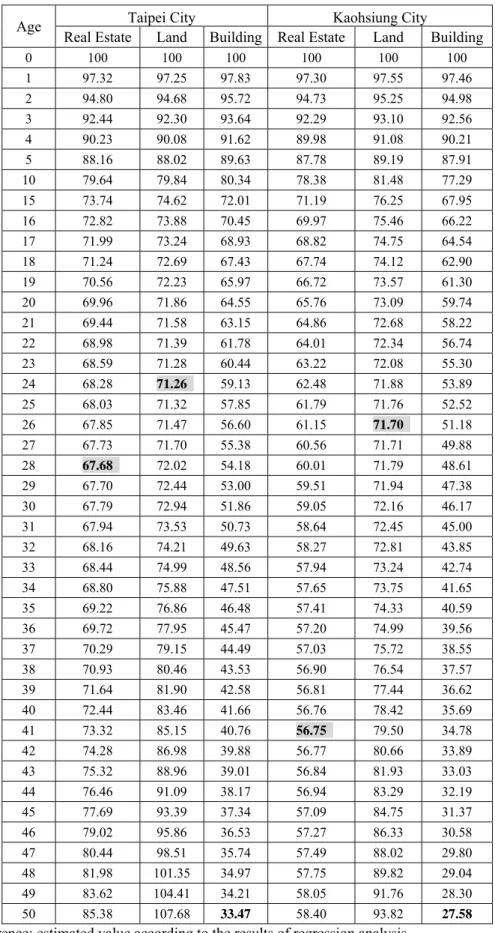
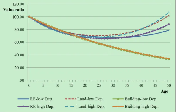
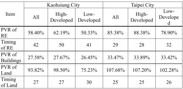
Depreciation declines the value of an asset over time. Most depreciation related studies have adopted building age and age-squared as independent variables in regression analysis, with both coefficients usually significant, showing that real estate value first decreases but then increases within a building’s residual economic life. The view that “real estate value constantly declines” is thus questioned. This study decomposed real estate as two components: a building and a plot of land. We used multi-regression analysis to address the depreciation of land, building, and real estate value in Taipei and Kaohsiung, Taiwan. The results showed an inverse depreciation of real estate and land values, with greater building age leading to greater land value and real estate value but lower building value, with certain regional differences.
Keywords: hedonic price model, real estate, economic depreciation
* Professor, Dept of Land Economics, National Chengchi University, [email protected]
5 Introduction
The value of assets decreases over time due to depreciation, such that new housing prices should be higher than existing housing prices in the real estate market. However, old apartment prices in Taipei, Taiwan, hit record highs recently due to the impact of urban renewal programs, such that the older the apartment was, the higher it was priced, even approaching the prices of newly built units on the market. That is, real estate value first decreases but then increases within its residual economic life. This situation, called inverse depreciation, is different from the general depreciation paradigm. Is this a special case or is it general? Does it happen only in urban renewal areas, or is it widespread in most regions?
Empirical research on real estate valuation is mostly based on hedonic price theory and adopts regression analysis. In hedonic price modeling, building age is usually used as the proxy variable of depreciation to analyze time variation of real estate value. In recent years, many empirical studies on the non-linearity of the age effect use building age and age squared variables, showing real estate value increases over time after an initial reduction of real estate values, or inverse depreciation, within its useful life (Malpezzi et al., 1987; Goodman and Thibodeau, 1995, 1997; Lee et al., 2005; Clapp and Salavei, 2010). Lee et al. (2005), Clapp and Salavei (2010), and Liang (2012a) pointed out that this increment was due to the real estate development value.
However, real estate is comprised of land and buildings. Because of physical deterioration, functional obsolescence, and external changes in economic conditions and other factors, building value generally depreciates over building lifespan, whereas the value of land is generally believed not to depreciate (Malpezzi et al., 1987;Smith, 2004;Fisher et al. 2005). Under the view that in real estate only buildings depreciate, real estate values derived from land and buildings should depreciate at lower rates than buildings, inverse depreciation of real estate value with building age should not occur. Should this phenomenon be reflected in valuation, and is inverse depreciation a prevalent phenomenon? Is it related to redevelopment value? Is it still true that land does not depreciate, and would the soon-to-be-demolished buildings contain re-development value and also exhibit inverse depreciation? These questions motivated this paper analyzing the role of internal real estate structure in inverse depreciation.
This study proposes to investigate and analyze the housing age effect from the perspective of land, building, and real estate and furthermore to clarify the impact of redevelopment value on real estate value. In addition, real estate redevelopment is
6
subject to external environmental influences and regional differences. Therefore, the inverse depreciation phenomenon exhibits spatial differences in redevelopment value.
To verify the above analysis, we intend to further analyze regional differences in the existence of the universality of the phenomenon of inverse depreciation.
To deepen the above investigation of inverse depreciation of real estate values, this study will conduct empirical analysis of residential real estate price data to verify the building age effect, namely, that housing prices vary with building ages, and regional differences therein.
Literature Review
Samuelson (1964), Hulten and Wykoff (1981), Baum (1991) pointed out that depreciation is the reduction of asset prices over time. Malpezzi et al. (1987) considered the hedonic price model the most widely applied among the observed age method, perpetual inventory method, and hedonic price methodology. Age, a depreciation proxy variable, is always adopted in the model with other factor variables. Moreover, Sirmans et al. (2005) found the age variable to be used to estimate price in almost all of 87 empirical articles reviewed. We will also use age as the key variable to analyze the depreciation effect in this study.
Empirical literature focuses on how to accurately estimate amount of depreciation (Malpezzi et al., 1987; Smith, 2004; Dunse and Jones, 2005; Fisher et al., 2005) as well as to explain the estimated age coefficient. Most studies have shown the nonlinearity of age effects (Hulten and Wykoff, 1981; Malpezzi et al., 1987; Coulson and McMillen, 2008; Goodman and Thibodeau, 1995, 1997).
Hulten and Wykoff (1981) showed willingness to pay for retail and industrial property and building depreciation to 2.02% to 3.61%. Malpezzi et al. (1987) demonstrated the various results on depreciation derived from different definitions, different models, or different databases. Therefore, they adopted a semi-logarithmic model in 59 metropolitan areas and demonstrated that depreciation rates did vary among these areas. Their results showed a decreasing deceleration situation such that the average depreciation rate decreased from 0.28% in the first year to 0.9% in the 20th year for owner-occupied real estate. However they did not proffer any theoretical explanations. Smith (2004) studied building and found depreciation rates from 0.5% to 7% in single-family housing, lower than the real estate average of the and with spatial variation in building depreciation. Fisher et al. (2005) also estimated multi-family depreciation rate at approximately 2.7% in the residential investment market. Building depreciation rate was approximately 3.25% if the real estate depreciation rate was
7
adjusted by the proportion of the overall real estate value accounted for by land. With an inflation rate of 2%, the nominal depreciation rate was approximately 5.25%. Willelmson (2008) used the interaction variable of location and age, showing that general depreciation rate was 0.77% and depreciation rate of poor maintenance real estate up to 1.10 %.
This literature shows that building is the object by which to estimate depreciation, but building price is difficult to acquire. Under the viewpoint that land is not depreciated (Malpezzi et al., 1987; Smith, 2004; Fisher et al., 2005), depreciation should be estimated at a lower rate, and bias exists when using real estate data. Therefore, Fisher et al. (2005), Lin and Jhen (2009), and Lin et al. (2011) accounted for building depreciation rate using the proportion of land price and real estate value. However, land does not depreciate, and land value is not, like buildings, are subject to decreases over time change. The proportion of depreciation constituted by land and buildings should change over time. Do such practices may overestimate building depreciation, and how should we deal with these problems of the inverse depreciation? Smith (2004) directly adopted building price as evaluated by an assessor, a direct analysis of the effective building depreciation and the approach adopted in of this study.
The empirical results of Hulten and Wykoff (1981) suggested that age depreciation changed in a nearly geometric, not linear, pattern. Subsequently, many residential studies adopted nonlinear depreciation analysis, convex to the original point and concave to the original point. Wolverton (1998) divided data into six groups and empirical results showed building age was convex to the original point, as initial depreciation accelerated to late depreciation type. However, the empirical evidence of Cannaday and Sunderman (1986) supports a path of depreciation for single-family houses in Illinois that is concave. Building depreciation exhibited a reverse sum of the annual path most closely approximating the path of the sinking fund method, initially less rapid than a straight-line. Taubman and Rasche (1969) and Jones et al. (1981), studied office real estate and had the same results.
To avoid limiting depreciation estimates and to understand nonlinear patterns, Malpezzi et al. (1987), Goodman and Thibodeau (1995, 1997), Smith (2004), and Wilhelmsson (2008) recommended using the age and age square or age cubic variables to capture changes in the price model. Housing age squared changes in the value of real estate, use of variables, or age cubic, decreased with the increasing age, and may increase after a hurdle age. That is, the age effect of the real estate value may be inverse depreciation. Inverse depreciation explores an impact not only on real estate depreciation but also on the building depreciation.
8
Because of inverse depreciation, Randolph (1988) thought it to be related to the vintage effect of housing age. Rubin (1993), Clapp and Giaccoto (1998) explained it by consumer preferences and rational expectations. Lee et al. (2005) indicated that with increase in the age of a building, real estate does not only generate depreciation but also updates the possibility for redevelopment. If there are economic benefits to development, to update expected net income by the capitalization of real estate will have a positive price impact. Therefore, with increasing age real estate values may first decrease and then increase. Based on a similar viewpoint, Clapp and Salavei (2010) established theoretically a model containing the value in use and redevelopment options as the basis of the empirical analysis.
The situation of real estate values increasing with building age and the aging of housing increases the possibility for redevelopment, and the age variables of the hedonic price model imply not only a negative depreciation effect but also reflect a positive effect of redevelopment with increasing age. Therefore, when the price function contains land value, in a building’s later life, land value increment is generated by the possibility of redevelopment and a price decline with the aging building will create bias. Therefore, it is necessary to clarify the age effect by analysis of land depreciation and building depreciation. In addition, Malpezzi et al. (1987), Smith (2004), and Fisher et al. (2005) suggested that land does not depreciate and that building value declines by physical deterioration and functional obsolescence. Basically, the real estate hedonic price model will show a lower depreciation rate. Malpezzi et al. (1987) and Smith (2004) also pointed out that different depreciation rates should be considered depending on whether land value is included in the dependent variable, but they did not indicate what the gap should be. Therefore, we try to observe changes and inverse depreciation separately in land value and building value from real estate value.
Except for depreciation estimate literature, some studies researched different properties, different years, or different regions in order to improve the accuracy of the estimates. Malpezzi et al. (1987) studied data quality and pricing models and found that obsolescence varies with location. Smith (2004) and Willelmson (2008) also agreed.
As for the causes of regional differences, Salway (1986) argued that depreciation is likely to be highest where land values are lowest. In other words, depreciation is lowest where the land component of rent is greatest. Because land value is unaffected by physical deterioration, the higher the land value proportion of real estate, the lower depreciation is. In general, depreciation will vary both within cities and within regions. Through appraisers’ professional judgments, Baum (1991) studied 125 industrial
9
properties in London and 125 office buildings in west London. He found the depreciation rate of industrial real estate located in the suburbs to be lower. Baum (1997) and Barras and Clark (1996) supported these results. Baum and Turner (2004) also pointed out that long-term tenant leases in office buildings would reduce management and property transactions, resulting in higher depreciation than the contrasting shorter lease ones.
Dunse and Jones (2005) considered that areas of highest accessibility and land values might also have lower depreciation. They tested their hypotheses by the use of hedonic regression analysis in five industrial property market areas in west central Scotland. However, it seemed at least in the case of Glasgow that the influence of property market dynamics had a more significant effect than land values. They found that spatial variation existed and that high land values slowed depreciation of industrial properties. These results were similar to those of Fraser (1993), who suggested that the high elasticity of supply would lead to a higher rate of depreciation. However, the empirical results of Lin et al. (2011) in Taipei showed depreciation to be different, the great location region being relatively slow. Liang (2012) also pointed out that the residual value rate of buildings is different in different regions.
The above literature agrees that there are spatial variations in depreciation, except that the causes are inconclusive. Inverse depreciation of real estate values may occur due to the possibility of redevelopment. The stronger the redevelopment potential, the higher the changes in regions, inverse depreciation should be more obvious.
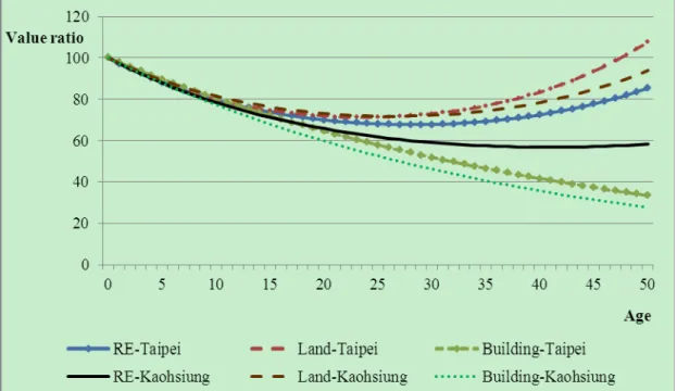
Based on the above discussion, we proposed the following hypothesis: 1. Inverse depreciation exists in real estate.
2. Inverse depreciation doesn’t exist in buildings but does exist in land.
3. Inverse depreciation is positively linked to the rate of property development and spatially varies with land value.
Model
The hedonic pricing model is widely used in real estate research. The model assumes that real estate price is comprised of the value of its different components. To analyze the depreciation of real estate, building, and land value, this study adopted the hedonic pricing model and used regression analysis to explore significant components that affect real estate value and to estimate their shadow prices to find the differences between each pricing model. For the hedonic regression pricing model, the natural log of the price will tend to be normal in distribution and reduce heteroscedasticity problems (Allison, 1999). The results of the semi-logarithmic model are more
10
consistent and relatively stable (Soderberg, 2002). Vanderford et al. (2005) also found the performance of the semi-logarithmic model to be better. Many studies have been analyzed using the semi-logarithmic model (Smith, 2004; Fisher et al., 2005; Chen and Yang, 2007; Wilhelmsson, 2008). Therefore, this study used the semi-logarithmic hedonic pricing model as the empirical model. The equation used is shown in equation (1): i k n 1 n j j ji n 1 j j ji 0 β X β D ε α ) i Ln(P
………(1) error term the stic characteri j the of t coefficien i unit of able dummy vari j the D i unit of variables random continuous j the erm constant t i unit of price the of log natural the th th th i j ji ji 0 i ε β X α ) Ln(PA real estate can be conceptualized as a bundle comprising of physical structure and a non-reproducible plot of land (Davis and Heathcote, 2007; Davis and Palumbo, 2008). Therefore this study individually uses the natural log of real estate price, building price, and land price as the dependent variable. The independent variables, mainly with reference to the prior studies, include continuous variables such as building area, lot area, floor area ratio, roads, distance to public facilities, and dummy variables such as structure, year, etc. (Smith, 2004; Sirmans et al., 2005; Lin and Jhen, 2009). The purpose of this study is to analyze the space-time effects of depreciation so that building age is the main independent variable. To observe inverse depreciation, this study used age and age square as independent variables. However, these two variables have collinearity problems in the regression analysis. Therefore, we adopted "age deviation" (agedev) and "the square of age deviations” (agedev2) as proxy variables of depreciation for the analysis of land and building value. As for the depreciation of buildings, since the economics implies that the longer the building is used, the lower the value will be, we only used “age” as the proxy variable. Descriptions of each variable are shown in Table 1.
11
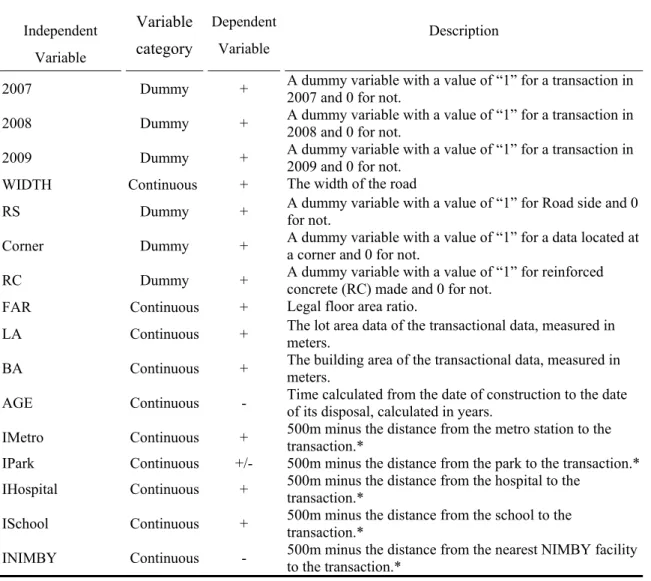
Table 1: The Variables Independent Variable Variable category Dependent Variable Description
2007 Dummy + A dummy variable with a value of “1” for a transaction in 2007 and 0 for not. 2008 Dummy + A dummy variable with a value of “1” for a transaction in 2008 and 0 for not. 2009 Dummy + A dummy variable with a value of “1” for a transaction in 2009 and 0 for not. WIDTH Continuous + The width of the road
RS Dummy + A dummy variable with a value of “1” for Road side and 0 for not. Corner Dummy + A dummy variable with a value of “1” for a data located at a corner and 0 for not. RC Dummy + A dummy variable with a value of “1” for reinforced concrete (RC) made and 0 for not. FAR Continuous + Legal floor area ratio.
LA Continuous + The lot area data of the transactional data, measured in meters. BA Continuous + The building area of the transactional data, measured in meters. AGE Continuous - Time calculated from the date of construction to the date of its disposal, calculated in years. IMetro Continuous + 500m minus the distance from the metro station to the transaction.* IPark Continuous +/- 500m minus the distance from the park to the transaction.* IHospital Continuous + 500m minus the distance from the hospital to the transaction.*
ISchool Continuous + 500m minus the distance from the school to the transaction.*
INIMBY Continuous - 500m minus the distance from the nearest NIMBY facility to the transaction.* Reference:Real estate newsletter of transaction prices, the conclusions from GIS.
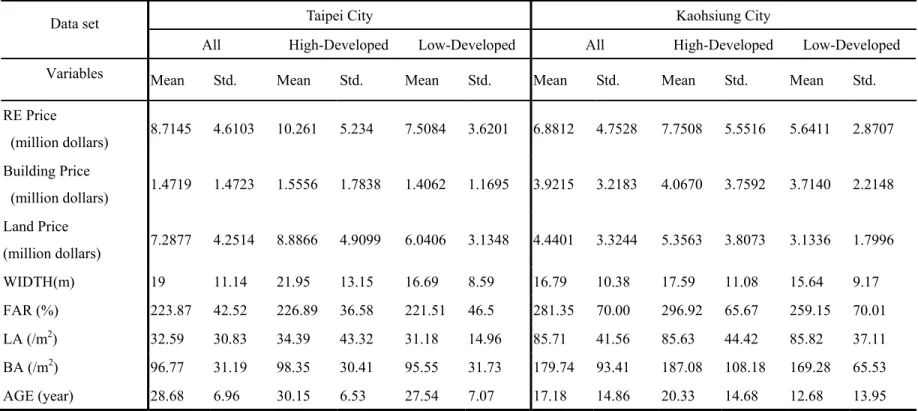
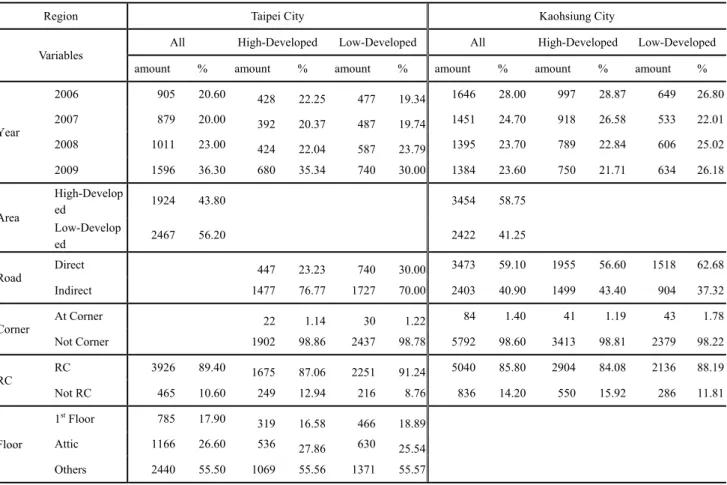
Data
In order to compare differences between depreciation of land and buildings, we have to separate land price and building price from real estate price. We follow the idea of Davis and Heathcote (2007) and Davis and Palumbo (2008) to calculate building price by the replacement cost after accounting depreciation and to calculate land price as the difference between the market value of real estate and depreciated building price. To reduce complexity, this study examined transactions of townhouses, for which it is not necessary to consider three-dimensional distribution premium rates when separating the prices. This may decrease the degree of deviation. In addition, the spatial context in this study is Kaohsiung City, where land price is relatively stable and transactions are sufficient so as to avoid the impacts of expectation and land price fluctuations. To verify inverse depreciation of real estate and to test for spatial