AN EFFICIENT APPROACH TO SOLVING THE MINIMUM SUDOKU PROBLEM
Hung-Hsuan Lin1 and I-Chen Wu1 Hsinchu, Taiwan
ABSTRACT
Since Sudoku was invented, it has been an open problem to find the minimum-clue Sudoku puzzles, also commonly called the minimum Sudoku problem. Solving the problem can be done by checking 5,472,730,538 essentially different Sudoku grids independently or in parallel. In the past, the program CHECKER, written by McGuire, required about 311 thousand years on one-core CPU to check these grids completely, according to our experimental analysis. This paper is to propose a more efficient approach to solving this problem. We design a new algorithm, named disjoint minimal unavoidable set (DMUS) algorithm, to help solve the minimum Sudoku problem more efficiently. After incorporating the algorithm into the program and further tuning the program code, our experiments showed that the performance was greatly improved by a factor of 128.67. Hence, it is estimated that it only takes about 2417 years to solve the problem. Thus, it becomes feasible and optimistic to solve this problem by using a volunteer computing system, such as BOINC.2,3
1. INTRODUCTION
Sudoku is a popular puzzle game invented by Harold Garns (cf. Mailer, 2008) in 1979 and has been popular and printed in daily newspapers, magazines, and websites since 2005. A Sudoku puzzle is played on a 9×9 grid which is divided into nine boxes each with 3×3 cells. In a puzzle, some digits between 1 and 9 are initially given on the grid as the clues.
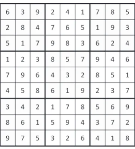
(a) (b) Figure 1: (a) A 17-clue puzzle and (b) its complete grid.
The aim of a Sudoku puzzle is to fill the 9×9 grid up from the initial grid of the Sudoku puzzle into a valid Sudoku complete grid, or in this paper simply called a complete grid, where each column, each row, and each box contains the distinct digits 1-9.
A Sudoku puzzle is called a valid Sudoku puzzle, or straightforwardly a valid puzzle, if it is solved by a unique complete grid. The program used to solve the puzzle is called a solver. Note that a puzzle that can
1
Department of Computer Science and Information Engineering, National Chiao Tung University, Hsinchu, Taiwan. Email: [email protected], [email protected].
2
Berkeley Open Infrastructure for Network Computing. 3
be solved by more than one complete grid is called a malformed puzzle, which is less interesting to Sudoku players. A valid puzzle with n clues initially is called an n-clue puzzle. Figure 1 (a) illustrates a 17-clue puzzle, while Figure 1 (b) shows the complete grid of this puzzle.
Most current published valid puzzles are clue puzzles with n more than 20. Roughly speaking, the n-clue puzzles are more difficult to solve for small n, and easier for large n. For example, if the number of clues is close to 80, most of these non-clue cells have only one choice, and therefore it becomes very easy to solve. Surely, this is not always the case as pointed out in Palánek (2011).
Now, an intriguing open question is: what is the minimum number of clues for a valid puzzle? This is the so-called minimum-clue Sudoku problem, or the minimum Sudoku problem. Currently, many 17-clue puzzles have been found. One of these puzzles is shown in Figure 1 (a). However, so far, no 16-clue puzzles have been found. Thus, the problem is still open. The approach to solving this problem is briefly described as follows.
For a given grid, we can easily generate more isomorphic grids described in Russell and Jarvis (2006) by the following operations.
Relabel digits. For example, relabel all 2s and 5s to 5s and 2s, respectively.
Permute single rows (columns) within the same box row (column), or permute box rows (columns). A box row (column) indicates the three boxes in the same rows (columns). For example, permute the first and second rows; permute the first box column (the leftmost three boxes) and the second box column (the middle three boxes).
Rotate and mirror boards.
An important assertion is: if a puzzle P with initial grid G is valid, then another puzzle P' with initial grid G' which is isomorphic to G is valid too. The puzzle P' is said to be isomorphic to P. For simplicity of discussion, let iso(G) denote the group of isomorphic grids generated from G. Note that G is also included in iso(G). From above, if a puzzle with initial grid G is valid, all the puzzles with initial grids in iso(G) are valid too.
The numbers of isomorphic grids in groups are usually enormous. For example, a complete grid may have up to 2*9!*68 = 1,218,998,108,160 isomorphic complete grids. Similarly, a valid puzzle such as the one in Figure 1 (a) normally has enormous isomorphic valid puzzles, too. Thus, it becomes less interesting to find valid puzzles which are isomorphic to some found valid puzzles. Currently, Royle (2007) collected 49,151 17-clue puzzles, each of which is not isomorphic to any others. These puzzles are called essentially different Sudoku puzzles.
According to Felgenhauer and Jarvis (2006), the total number of complete grids is 6,670,903,752,021,072,936,960. In fact, many of them are isomorphic. The total number of distinct isomorphic groups is 5,472,730,538, according to Russell and Jarvis (2006). Fowler (2007) also generated 5,472,730,538 complete grids, one for each isomorphic group. These complete grids are essentially different Sudoku grids, and are called primitive grids in this paper. Two features of primitive grids are as follows.
1. Each complete grid is isomorphic to one of these primitive grids. 2. Each primitive grid is not isomorphic to any other primitive grids.
An important approach to solving the minimum Sudoku problem is to investigate exhaustively all these primitive grids only to check whether 16-clue puzzles exist in these primitive grids or not. The approach must be able to find one 16-clue puzzle, if there exists a 16-clue puzzle, for the following reason. Assume that some 16-clue puzzle P can be solved with a unique complete grid G. From the first feature, there exists one and only one primitive grid G', isomorphic to G. This implies that there exists a 16-clue puzzle P' solved by the complete grid G' uniquely. Namely, we can translate the initial grid of puzzle P into that of P' by using the same transformation from G to G'. Thus, the puzzle P' should be found when the primitive grid G' is investigated.
Using this approach, McGuire (2006) wrote a program, named CHECKER, to help solve this problem. Given a number n and a complete grid, the program checks whether there exist n-clue puzzles which can
be solved with the complete grid, and outputs the found n-clue puzzles, if any. Hence, we can solve the minimum Sudoku problem by using CHECKER to search 16-clue puzzles from all the 5,472,730,538 primitive grids.
This approach has two advantages. First, the program does not need to investigate isomorphic complete grids redundantly. Second, these primitive grids can be checked independently. That is, they can be investigated in parallel.
However, the total computation time for solving the problem is still too high. McGuire said (cf. Delahaye, 2006) that none were near to proving whether there is a 16-clue puzzle or not. He estimated this as follows (cf. Delahaye, 2006). Assume that searching a grid might be doable in one minute on a powerful computer. Then, at that rate the endeavour would take 10,380 years. Even distributed on 10,000 computers, it would take about one year. Finally, he added a comment: “We really need a breakthrough in our understanding to make it feasible to search all the grids.”
According to our experiment (see Section 4), the program CHECKER actually required on average about 1792.31 seconds to check a primitive grid on one core of a computer equipped with the CPU, Intel(R) Xeon(R) E5520 @ 2.27GHz. Thus, for 5,472,730,538 primitive grids, it would take about 311,000 years. The total time was therefore too long.
In this paper, we propose a new approach to solving the problem more efficiently. We design a new algorithm, named DMUS algorithm, incorporate it into the program CHECKER, and make some more tunings on the program. According to our experiment (see Section 4), the modified program could check one on the average on one core of a computer in 13.93 seconds. Thus, it would only take about 2417 years to check all 5,472,730,538 primitive grids.
Using the modified program, it becomes more feasible to solve the problem on top of BOINC (2003). BOINC is a middleware framework for volunteer computing. Volunteer computing is attractive in the sense of supporting huge amount of free resources including computation and memory, such as idling desktops or notebooks. In the past, many projects, such as SETI@HOME (Anderson et al., 2002) and the Great Internet Mersenne Prime Search (1996), successfully used volunteer computing to solve problems based on top of BOINC. Recently, some projects in Wu et al. (2009, 2010a, 2010b) designed new volunteer computing systems to solve game problems. As for Sudoku, a project (2007) which seemed to use the original CHECKER attempted to solve the Sudoku problem on top of BOINC. However, it seemed that the project did not continue. Encouraged by the improvement shown in this paper, the authors of this paper were initiating another Sudoku project (2010).
This paper is organized as follows. Section 2 describes traditional approaches for the minimum Sudoku problem including the program CHECKER. Section 3 describes our new approach. Section 4 does experiments for analysing the performance improvements by our approach. Section 5 makes concluding remarks. A preliminary version of this paper was in Lin and Wu (2010). When compared with that version, this paper additionally includes the improved DMUS algorithm in Subsection 3.2, the design of Phase 1 in Subsection 4.2 and comprehensive experiments in Section 4.
2. TRADITIONAL APPROACH
Solving the minimum Sudoku problem is a quite difficult job as described above. Most researchers tend to seek 16-clue or 17-clue puzzles at random, instead of searching all cases exhaustively. In case that there exists some 16-clue puzzle, the 16-clue puzzle implies the existence of another 65 17-clue puzzles by simply filling one more cell on the 16-clue puzzle. Moreover, if one of the 65 17-clue puzzles is found, then we can easily find the 16-clue puzzle by removing one clue and checking whether or not it is still valid. Most researchers seek 17-clue puzzles in this approach.
The rest of this section is as follows, Subsection 2.1 describes the traditional approaches of finding more 17-clue puzzles, while Subsection 2.2 describes the traditional approaches of checking whether or not 16-clue puzzles exist.
2.1 Finding 17-clue Puzzles
One of the most popular algorithms of finding new 17-clue puzzles is called gene restructuring (see Huang, 2009). This algorithm starts with an n-clue puzzle and then performs the following operation. First, remove p existing clues on the puzzle, and then add q clues back to the puzzle. For simplicity, let – p+q indicate such an operation.
We introduce two common methods from the Sudoku Forum (2009) to obtain more 17-clue puzzles from the existing valid puzzles as follows.
1. Do –k+k operations from 17-clue puzzles.
2. Do the following from n-clue puzzles, where 18 ≤ n ≤ 23. a. Repeat –2+1 operations until 18-clue puzzles are obtained.
b. Then, repeat –1+1 operations many times to obtain more 18-clue puzzles. c. Finally, do one –2+1 operation to obtain more 17-clue puzzles.
The first method starts with 17-clue puzzles and does a –k+k operation to obtain new 17-clue puzzles. Running with k ≤ 2 is very fast, while it takes much longer time with k 4.
The second method starts with n-clue puzzles where 18 ≤ n ≤ 23, and repeats –2+1 operations until it gets 18-clue puzzles. Also it does an extra –1+1 operation many times on the 18-clue puzzles to obtain more 18-clue puzzles. Finally, a –2+1 operation is used on these 18-clue puzzles to obtain 17-clue puzzles. Both methods above are quite useful to find 17-clue puzzles. Many of the 49,151 17-clue puzzles were obtained in this way. However, since no 16-clue puzzles were found, they failed to conclude whether or not any 16-clue puzzles exist.
2.2 Checking All 16-clue Puzzles
A second approach to solving the minimum Sudoku problem is to search exhaustively for 16-clue puzzles. This can be done by the program CHECKER, written by McGuire (2006). This program was motivated when Royle (cf. McGuire, 2006) found a special complete grid shown in Figure 2, where we can find exactly 29 17-clue puzzles. That is, these 29 17-clue puzzles can be solved uniquely with this complete grid. Since a 16-clue puzzle could produce 65 17-clue puzzles as describe above, it is more likely that this complete grid contains a 16-clue puzzle, though no other 16-clue puzzles have been found from this puzzle by CHECKER.
Figure 2: The complete grid with 29 17-clue puzzles.
Given a complete grid and a number n, the program CHECKER runs the following two phases. Phase 1 is to search the grid for unavoidable sets, defined in Subsection 2.2.1. Phase 2, described in Subsection 2.2.2, is to use these unavoidable sets to search n-clue puzzles.
2.2.1 Phase 1: Unavoidable Sets and Finding Unavoidable Sets
In a complete grid, an unavoidable set is a set of cells on which the digits can be permuted to form another distinct complete grid. In other words, if we remove all the digits in an unavoidable set from the complete grid and let the remaining digits form a new puzzle, then the new puzzle can be solved with more than one complete grid. For example, for a complete grid including the digits shown in Figure 3, the four bolded digits, two 1s and two 2s, in the upper left corner form an unavoidable set. The complete grid is transformed to another complete grid by exchanging the 1s and 2s in this unavoidable set. In fact, all bolded 4s and 5s form one unavoidable set; all bolded 6s, 7s, 8s, and 9s form one; and all of these 1s, 2s, 4s, and 5s also form one. From the definition, we have the following assertion, which is important in Phase 2 of CHECKER.
Figure 3: Three minimum unavoidable sets.
Assertion 1. Assume P to be a valid puzzle uniquely solved by a complete grid G. For each unavoidable set in G, at least one of the cells in the unavoidable set must be a clue in P.
An unavoidable set S is called a minimal unavoidable set, or simply called a MUS in this paper, if there exist no other smaller unavoidable sets S' ⊂ S. For example, in Figure 3, there are three MUSs: one with all bolded 1s and 2s, one with all bolded 4s and 5s, and one with all bolded 6s, 7s, 8s, and 9s. The unavoidable set with all bolded 1s, 2s, 4s, and 5s is not a MUS. In this example, the smallest size of MUSs is four and the second smallest size is six. In fact, four is also the smallest size among all MUSs. Here, we introduce two approaches (the remove-region approach and the brute-force approach) used in CHECKER to find MUSs from a complete grid. They are explained in the following two subsections respectively.
Remove-Region Approach
The first approach is called the remove-region approach. It quickly finds the MUSs in a designated region of a complete grid. The approach performs the following four steps.
1. Remove the digits from the designated region of a complete grid G, and let the remaining digits form a new puzzle P.
2. Use a solver to solve P, many complete grids.
3. For each of the solved complete grids, the cells with different digits from those in G form an unavoidable set.
(a) (b)
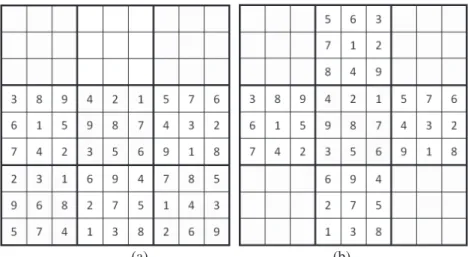
Figure 4: Removing a region of digits, (a) one box row and (b) 2x2 boxes, from a complete grid.
Figure 5: Another solved complete grid.
Let us illustrate the approach by the complete grid, denoted by G, shown in Figure 1 (b). By using the approach, remove the upper box row (the upper three boxes) from the complete grid G as a puzzle as shown in Figure 4 (a). Then, use a solver to solve the new puzzle. Surely, the original G must be one of the solved complete grids. Another one of the solved complete grids is shown in Figure 5, where the digits on the gray cells are different from those in the original G. Obviously, these gray cells form an unavoidable set, which is also a MUS since there exist no smaller unavoidable sets.
In the remove-region approach, the program CHECKER tried to remove three kinds of regions. The first kind is to remove a box row or a box column as shown in Figure 4 (a). Since there are three box rows and three box columns in a Sudoku grid, CHECKER needs to check six times for this kind of regions. The second kind is to remove 2x2 boxes as shown in Figure 4 (b). For this kind of regions, CHECKER needs to check nine times for a Sudoku grid. The third kind is to select three distinct digits, say 1, 2, and 3, and then remove all the 1s, 2s, and 3s in the complete grid. For this kind of regions, CHECKER needs to check C(9,3) (=84) times for a complete grid.
The advantages of the remove-region approach is to find quickly all the MUSs in a designated region, regardless of the sizes of MUSs, sometimes up to 20 or more. However, the drawback of this approach is that some MUSs with small sizes cannot be found. For example, some MUSs with sizes about 10 cannot be found in this approach. Note that the search in Phase 2, described in the next subsection, performs more efficiently for smaller size MUSs.
Brute-Force Approach
The second approach is called the brute-force approach. It uses a kind of brute-force method that is to search exhaustively all MUSs with different sizes, starting from 4 (the smallest size of MUSs). The approach is as follows. An initial set of MUSs with different sizes is prepared in advance, such as the one
with all 1s and 2s in Figure 3. For each of these MUSs, the method checks all of its isomorphic MUSs and then finds all of them matched in the complete grid. A MUS is said to be isomorphic to another MUS, if both are the same after we relabel digits and rotate/mirror columns or rows of one MUS such as described in Section 1. Surely, the MUSs in the initial set are not isomorphic to one another.
The advantage of the brute-force approach is that one can find MUSs with small sizes that cannot be found in the above approach. In CHECKER, most MUSs4 with sizes 12 or less were prepared in this approach.
The drawback of the approach is that checking all the isomorphic MUSs is performed inefficiently since one MUS has many isomorphic MUSs but a complete grid contains only a few of them. Since CHECKER took much longer times in Phase 2 (about 1754.89 seconds for a primitive grid, described in greater details in Section 4), the overhead incurred by the brute-force approach becomes negligible. Thus, the brute-force approach is also used in CHECKER.
2.2.2 Phase 2: Searching n-Clue Puzzles
Phase 2 is to use a tree search to find n-clue puzzles based on the MUSs found. By Assertion 1 described above, for each MUS, at least one clue in a valid puzzle must be located on one of cells in the MUS. Thus, given a number n, a complete grid G, and a set of MUSs, the program CHECKER in this phase is to find n-clue puzzles by recursively calling the tree search routine, named ProcessTuple(n, G, Xcur, C),
where Xcur is the set of active MUSs and C is the set of clues being chosen. A MUS is called active in this
paper, if none of cells in the MUS are chosen as clues (in C) yet, and inactive, otherwise. Initially, all MUSs are viewed as active MUSs, and there are no clues initially. The routine is described as follows. Routine ProcessTuple(n, G, Xcur, C):
1. If there exists at least one active MUS in Xcur, do the following.
a. If the number of clues, denoted by |C|, is already n, return without any puzzles found.
b. If |C| < n, find the active MUS, S, with the smallest size of cells. For each cell c in S, do the following.
i. Choose c as a clue, and add it into C.
ii. Update Xcur according to c. Namely, remove all active MUSs containing c from Xcur.
iii. Recursively call the routine.
2. If there exists no active MUSs, that is, the set Xcur is empty, do the following.
a. If |C| = n, check whether the puzzle with these n clues is valid or not. If valid, return this puzzle, an n-clue puzzle. If not, simply return without any puzzles found.
b. If |C| < n, repeatedly perform the operations 1.b.i to 1.b.iii for each non-clue c ∉ C on the grid G. At Step 1, the routine checks whether there exists at least one active MUS in Xcur, and performs, if so, the
substeps 1.a and 1.b as follows. Consider the case that the routine has chosen n clues and at least one of MUSs is still active, not containing any clues. Then, the chosen n clues do not form a valid puzzle according to Assertion 1. Thus, no more search is required, as described in Substep 1.a.
In the case that the routine has chosen less than n clues (as described in Substep 1.b), choose one MUS S for further search. For each cell in S, add it into C, update the set of MUSs Xcur accordingly, and search
more n-clue puzzles by recursively calling the routine itself. Note that the routine chooses the MUS with the smallest size of cells, since the one with less cells will expand a less number of subtrees. For example, in the complete grid given in Figure 6, if the cell with digit 6 at (5, 1)has been chosen, the routine finds another MUS with size 4 next, marked as gray in the figure, chooses one of these cells in the MUS as a clue, say the cell with digit 1 at (2, 5), and then recursively calls the routine itself to find more.
4
CHECKER prepares 47 kinds of MUSs for size 10, 44 for size 11, and 417 for size 12 in the initial set without proving that those are all.
Figure 6: The search tree in Phase 2 of CHECKER.
At Step 2, the routine performs Substeps 2.a and 2.b when no more active MUSs exist. In the case that the routine has chosen n clues (Substep 2.a), a solver is used to check whether the puzzle with the n clues is valid. If the puzzle can be solved with at least two distinct complete grids, the solver reports invalid. Otherwise, the solver reports valid, that is, a puzzle with n clues has been found.
In the case that the routine has chosen less than n clues (Substep 1.b), it becomes more promising to find n-clue puzzles. In this case, we need to check all non-clue cells by recursively performing the operations 1.b.i to 1.b.iii to search all n-clue puzzles.
The above routine needs to maintain the set of active MUSs efficiently. The maintenance includes the following two important operations, (a) finding the active MUS with the smallest size of cells, and (b) removing all MUSs containing a designated cell (chosen as a clue).
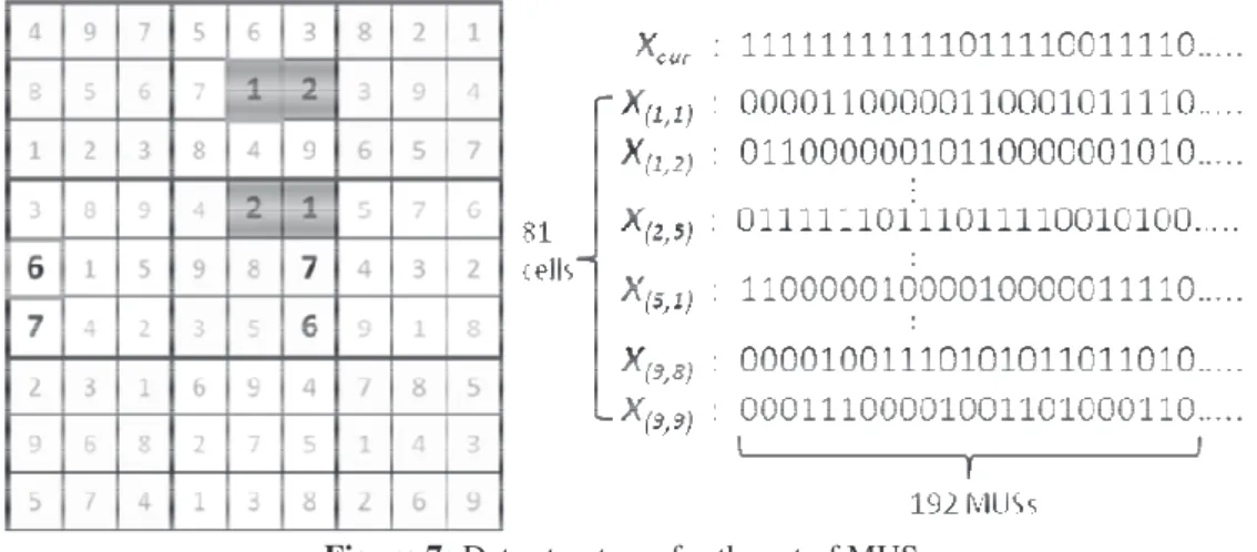
In the program CHECKER, the bit set data structure was used to implement the set of active MUSs, Xcur, as
shown in Figure 7. Let each bit in the data structure be corresponding to a designated distinct MUS. Namely, the ith bit with 1 indicates that the ith MUS is inactive, while the ith bit with 0 indicates that the ith MUS is active. It is the same when switching the representation of the values 0 and 1. Thus, for 192 MUSs, the default setting of CHECKER, the data structure requires 6 words each of 32 bits.
Figure 7: Data structures for the set of MUSs.
For operation (a), we can arrange the MUSs with small sizes to the front. For example, the MUSs with size 4, if any, are arranged to the front of bits of Xcur. So, if we want to find the active MUS with the
smallest size, we simply scan bits of Xcur from the front to rear and find the first bit with 0 (indicating
active). For example, if there exists some active MUS with size 6 and no active MUSs with size 4, we will find a MUS with size 6 by the scanning.
For operation (b), for each cell c, we initialize a set of MUSs Xc that contain the cell c. If we choose the
structure, we can easily use bitwise operations to remove the MUSs from the set of active MUSs easily. Let Xc be also implemented by a bit-set data structure. The ith bit in Xc is set to 1 to indicate that the ith
MUS contains the cell c, and 0, otherwise. For example, in Figure 7, if we choose one more cell with digit 1 at (2,5) to be a clue, Xcur becomes the value of performing an OR operation on the original Xcur and
X(2,5). Since a Sudoku grid contains 81 cells, only 81 Xc need to be initialized.
From the above, it can be shown that all the n-clue puzzles, if any, can be found by CHECKER. In addition, some more optimizations are executed by this program. For example, the same set of clues are not searched again. Namely, if the routine selects the clue at (5,1) and then at (6,1), the routine will not search again in the sequence, selecting the one at (6,1) and then at (5,1).
3. DMUS ALGORITHM
As described in Section 1, it would take a huge amount of time to solve the minimum Sudoku problem by CHECKER. In this section, we design a new algorithm in Phase 2, named Disjoint MUSs (DMUS) algorithm, and tune the code to improve the performance of CHECKER. The details of code tuning in both two phases are omitted in this paper. This section focuses on the DMUS algorithm. Subsection 3.1 proposes the basic DMUS algorithm, while Subsection 3.2 proposes the improved DMUS algorithm. 3.1 Basic DMUS Algorithm
The basic DMUS algorithm improved the program CHECKER by modifying Step 1.b, described in Subsection 2.2.2. In Step 1.b, an initial operation is added to find r+1 disjoint active MUSs. Let r denote n–|C|, representing the number of remaining clues to be chosen, where |C| is the number of clues in C. A set of MUSs are called disjoint MUSs, if any two of these MUSs do not overlap (namely, any two do not contain the same cells). An important assertion related to disjoint MUSs is described as follows.
Assertion 2. Use the program CHECKER to find n-clue puzzles as described in Subsection 2.2.2. If there exists at least r+1 disjoint active MUSs as above, then there exist no n-clue puzzles with C5.
From Assertion 1 in Section 2, for each MUS, a valid puzzle must include at least one clue in the MUS. Since there exist at least r+1 disjoint active MUSs in addition to the clues in C, a valid puzzle with C must also contain at least r+1 disjoint clues, each from one distinct MUS. Thus, the number of clues in the valid puzzle must be at least |C|+(r+1) = |C|+(n–|C|+1) = n+1. This implies that there exist no n-clue puzzles with C, that is, Assertion 2 is satisfied.
Given a set of MUSs, the problem of finding the largest number of disjoint active MUSs can be reduced to the maximum clique problem (cf. McGuire, 2006). However, the maximum clique problem is NP-complete (Berman and Schnitger, 1989). Since it is intractable to find a maximum clique, it is also intractable to find the largest number of disjoint active MUSs via finding the maximum clique.
In the basic DMUS algorithm, we use a greedy algorithm to find r+1 disjoint active MUSs one by one without exhaustively searching all kinds of disjoint active MUSs, such as backtracking. The algorithm repeatedly performs the following two operations until r+1 disjoint active MUSs are found or no more disjoint active MUSs exist.
1. Choose one additional disjoint active MUS with the smallest size in Xcur.
2. Add the chosen MUS into the set of disjoint MUSs.
In the first operation above, we choose the one with the smallest size, since it is more likely to find r+1 disjoint active MUSs in this way. This operation is the same as operation 1.b in Subsection 2.2.2, and therefore can be implemented by using the same bit operation.
In the second operation, we add the chosen MUS, S, into the set of disjoint MUSs. We can implement it by pretending to select all cells in S as clues. Namely, we remove all the active MUSs in Xc from Xcur for
all cells c in S. Thus, all the next chosen MUSs must not contain any cells in S. For example, in Figure 8,
5
after we find the active MUS A, we can update the Xcur by removing Xc for all the four cells c in A. Thus,
the next chosen MUS must not have any intersected cells with MUS A.
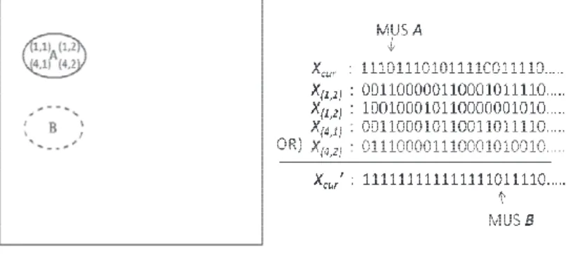
Figure 8: Finding the next disjoint MUS.
In fact, the operation can be easily improved by making a union of Xc for all cells c in S in advance. At
the beginning of Phase 2 (or the end of Phase 1), for each MUS S, we make an XS which is the value of
doing the OR operation on Xc for all cells c in S. Thus for the case in Figure 8, after selecting MUS A, we
can update Xcur by making one OR operation for XA, instead of four Xc for all cells c in A.
In the case that r+1 disjoint active MUSs are found by using the above algorithm, we can prune the whole subtree, since there exist no n-clue puzzles according to Assertion 2. In the case that r disjoint active MUSs or less are found, the program goes back to the normal operation 1.b (in Subsection 2.2.2) to traverse the whole search subtree.
3.2 Improved DMUS Algorithm
This subsection further improves the basic DMUS algorithm described in the previous subsection in the case that exactly r disjoint active MUSs are found. Let the r disjoint active MUSs be S1, S2, … , Sr.
Combining both Assertion 1 and Assertion 2, we obtain the following assertion.
Assertion 3. Use the program CHECKER to find n-clue puzzles as described in Subsection 2.2.2. Assume one finds r disjoint active MUSs, denoted by S1, S2, … , Sr, as above. An n-clue puzzle with C must
contain at least one of the cells as clues in each Si with 1 ≤ i ≤ r.
Based on the assertion, a straightforward search tree needs to search about ∏i |Si| puzzles, where |Si| is the
size of Si. In general, the performance is related to the sizes of these Si. So, if these sizes are reduced, the
performance is further improved.
In this subsection, we propose a new method to reduce the size of each Zi, subset of Si, while maintaining
Assertion 4 (below), similar to Assertion 3, where Z1, Z2, …, Zr are disjoint sets of cells, initialized to S1,
S2, …, Sr, respectively.
Assertion 4. From the above, for each set Zi, where 1 ≤ i ≤ r, an n-clue puzzle with C must contain at
least one of the cells in the set as clues.
Assertion 4 is satisfied initially from Assertion 3. The new method to reduce the size of each Zi is
described in the following routine. Routine Shrink(i):
1. Let Z = (Z1 ∪ Z2 ∪…∪ Zr) − Zi.
2. For each active MUS S (without containing any clues in C) disjoint with Z, let Zi = Zi ∩ S.
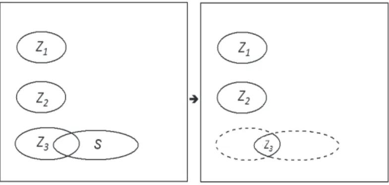
Let us illustrate the idea by an example in Figure 9. Assume that r is three, and assume to find the three active disjoint MUSs S1, S2, and S3. As described above, Z1, Z2, and Z3 are initialized to S1, S2, and S3, and
Figure 9: Shrink the Z3 to the intersection of Z3 and S.
Since r is three, we need to choose three more clues, each of which must be located in S1, S2, and S3,
respectively. Let us use Shrink(3) to shrink Z3. In the routine, Z is initially set to Z1 U Z2. Assume that
some other active MUS S is disjoint with Z (both Z1 and Z2) as shown in the left of Figure 9. The set Z3 is
shrunk to be the intersection of the original Z3 and S as shown in the right of Figure 9.
Assertion 4 still holds for the new Z3 together with both Z1 and Z2 for the following reason. Assume for
contradiction that none of clues in an n-clue puzzle with C are located in the new Z3. From above, the
clue that is located in the original Z3 must be outside the MUS S. Since S is an active MUS disjoint with
both Z1 and Z2, none of clues are located in S. Thus, according to Assertion 1, the n-clue puzzle is not
valid, contradicting the assumption. This shows that the clue in the original Z3 must be in the new Z3, too.
Based on the above illustration, it can be easily derived that Assertion 4 still holds after performing Shrink(i). Namely, if Assertion 4 holds currently, then it will also hold after Shrink(i). By induction, Assertion 4 is maintained by repeatedly performing the routine Shrink.
Since the set Zi may shrink after Shrink(i), it becomes very likely to shrink other Zj further, where j≠ i.
Therefore, it is reasonable to perform Shrink repeatedly many times.
Many strategies can be used to perform Shrink repeatedly. For the example in Figure 9, we may choose the sequence, Shrink(1), Shrink(2), and then Shrink(3), or the sequence, Shrink(3), Shrink(2), and then Shrink(1). We may even choose the sequence, Shrink(1), Shrink(2), Shrink(3), Shrink(2), and then Shrink(1). More discussion is given in our experiments in Subsection 4.4.
In the case that some Zi becomes empty after the routine Shrink(i) is finished, we can easily derive from
the above that none of n-clue puzzles exist. Thus, we can prune the whole subtree at Step 1.b in the routine ProcessTuple (in Subsection 2.2.2), like the case that we have r+1 MUSs. In fact, the case of r+1 disjoint active MUSs can be viewed as a special case. Let Z1, Z2, …, Zr be the first r disjoint active
MUSs. Then, for Shrink(r), the set Zr becomes empty when choosing the last disjoint MUS Zr+1 as S.
Namely, Zr = Zr ∩ S = Zr ∩ Zr+1 is empty.
In the case that none of Zi becomes empty, we choose the one, say Zj, with the smallest size among all Zi,
and then continue the search in the operation 1.b by using Zj, instead of the original S1, the MUS with
smallest size. Thus, the branching factor of the search tree becomes smaller, and therefore the size of the whole search tree is greatly reduced.
Besides the algorithm above, we also did many other tunings on the modified program. The details of these tunings are omitted in this paper.
4. EXPERIMENT
We implemented the basic DMUS algorithm and the improved one as described in the previous section by modifying the program CHECKER. For performance analysis, all experiments were done on a personal computer equipped with the CPU, Intel(R) Xeon(R) E5520 @ 2.27GHz. In the rest of this paper, one core indicates the above computing power.
Since it took a long time for the original program CHECKER to find 16-clue puzzles from one primitive grid, we only chose 100 at random among the 5,472,730,538 primitive grids (generated by the Fowler’s (2007) program as mentioned above) as our benchmark for comparisons. The 100 primitive grids are listed in the webpage of the Sudoku project on BOINC (2010). For clarity of discussion, all experimental results in the rest of this section are given on the average of the chosen 100.
In the rest of this section, Subsection 4.1 analyses the performance results in Phase 2 by comparing different versions of the program. Subsection 4.2 shows the results of the modified program in Phase 1. Subsection 4.3 shows the overall performance by including tuning the performances in Phase 1 of the program using different techniques. Subsection 4.4 compares the performances for different sequences of Shrink(i) in the DMUS algorithm. Subsection 4.5 shows the number of nodes in each level of Phase 2 in CHECKER.
4.1 The Results in Phase 2
In addition to the DMUS algorithm described in Section 3, our implementation also included many tunings, which are either omitted or briefly described due to tediousness. In this subsection, we analyze the performances of the following versions of implementations.
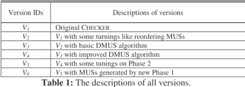
Version IDs Descriptions of versions V1 Original CHECKER
V2 V1 with some turnings like reordering MUSs V3 V2 with basic DMUS algorithm
V4 V3 with improved DMUS algorithm V5 V4 with some tunings on Phase 2 V6 V5 with MUSs generated by new Phase 1
Table 1: The descriptions of all versions.
As shown in Table 1, all versions are described as follows. The original version of CHECKER is denoted by V1. Before implementing the basic DMUS algorithm, we tuned the program by reordering the
selection sequence of MUSs based on the sizes of MUSs and some other factors. After the tuning, the version is denoted by V2. The version is denoted by V3 after incorporating only the basic DMUS
algorithm into V2. Similarly, the version is denoted by V4 after incorporating only the improved DMUS
algorithm into V3. Then, we made additional tunings in Phase 2 of version V4, such as reordering the
sequences of MUSs and cells in MUSs during search; this version is denoted by V5. All the MUSs used in
the versions V1 to V5 were generated by the original CHECKER. The last version, denoted by V6, was the
same as V5, except that all the MUSs were generated in Phase 1 by our modified program. Since this
subsection focuses on the performances in Phase 2, the version V6 will be discussed in the next
subsection, not in this subsection.
Table 2 shows the averaged time of solving one primitive grid in Phase 2 in each version. In this table, we also tried different numbers of MUSs, such as 128, 192, 256, 320, 384, 448, and 512. As described above, all the MUSs used in the versions V1 to V5 were generated by the original CHECKER. According to
our experiments, about 358.4 MUSs were generated on average for a primitive grid. The versions V1 and
V2 did not run the cases for 384 MUSs or higher because the original CHECKER did not support them.
# of MUSs 128 192 256 320 384 448 512 The fastest Speed-up V1 2093.41 1754.89 1811.61 1926.37 1754.89 1.00 V2 1210.80 586.75 576.87 617.95 576.87 3.04 V3 818.03 93.65 52.77 44.51 47.65 50.86 52.75 44.51 39.43 V4 704.57 64.76 25.68 19.95 19.54 20.83 21.74 19.54 89.81 V5 705.98 59.51 18.85 13.00 12.45 12.71 13.07 12.45 140.96 V6 730.69 56.01 19.06 13.28 12.84 12.93 13.42 12.84 136.67
Table 2: The averaged time of solving one primitive grid in Phase 2 for each version.
In general, the more MUSs we used, the smaller search tree. Assume that more MUSs are available in Phase 2. Then, it is more likely to choose Substep 1.a to stop calling recursively. Thus, it makes the
search tree smaller. Besides, more active MUSs may also help prune the search tree in our DMUS algorithm.
Searching smaller trees usually tends to raise the performance, but it is also noted that more MUSs may incur extra overhead. From Table 2, we observe the following: The version V1 reached the best
performance for 192 MUSs, version V2 for 256, version V3 for 320, and version V4 and V5 for 384. When
the numbers of MUSs decreased from the above numbers (for the best performances), the corresponding performances went down. However, when the numbers of MUSs increased from the above values, the performances also went down due to the overhead incurred by the large set of MUSs.
Comparing all versions by their best performances, we obtained that the speedups with respect to the version V1 were 3.04, 39.43, 89.81, and 140.96 respectively for versions V2 to V5. More specifically, the
DMUS algorithm improved significantly the performance by a factor of 29.54 (through V2 to V4),
especially the basic DMUS algorithm improved by a factor of 12.97 (through V2 to V3). Except the
DMUS algorithm, the other tunings (through V1 to V2 and through V4 to V5) improved by a factor of 4.77.
4.2 The Results in Phase 1
In this subsection, we want to discuss the experimental results in Phase 1. As described in Subsection 2.2.1, Phase 1 of the original CHECKER used both the remove-region approach and the brute-force approach to find MUSs.
According to our experiments, for the remove-region approach, the original CHECKER found the MUSs in the designated regions and kept the MUSs with sizes 14 or less. The program with this approach ran very fast in about 0.5 seconds in Phase 1, and it was able to find only about 222.54 MUSs on average for a complete grid, among which 139.41 have sizes 12 or less.
In fact, the program also used the brute-force approach to search the MUSs with size 12 or less and was able to find about 358.4 MUSs on average for a complete grid, but it took much longer time, about 37.4 seconds, to find MUSs for a complete grid. Since the original CHECKER took a much longer time in Phase 2 (about 1754.89 as shown in the previous subsection), the computation time, 37.4 seconds, is negligible. Thus, it is more important for the program to use the above approach to find higher quality MUSs. However, since our DMUS algorithm improves the performance significantly in Phase 2 as described in the previous subsection, the computation time for Phase 1 also becomes critical. Thus, we need to improve the performance in Phase 1. Our approach is to investigate the remove-region approach instead of the brute-force approach.
We improved the remove-region approach by magnifying the removed regions. In addition to removing three distinct digits, the third kind of regions described in Subsection 2.2.1, we also removed all combinations of regions with four boxes, and some more combinations to ensure to find all the MUSs with size 10 or less. After the tuning, we successfully reduced the averaged computation time in Phase 1 for each primitive grid from about 37.42 seconds down to about 1.09 seconds, while still obtaining high quality MUSs for Phase 2.
For the quality of MUSs, let us compare the performances of both versions V5 and V6 in Phase 2, since
both versions were the same except for the used MUSs. From Table 2, most performances in V6 in Phase
2 were, in general, slightly worse than those in V5. In the case of 384 MUSs, where both versions reached
the best performance, the performance in V6 was reduced by only about 3% in Phase 2 when compared to
that in V5. The averaged computation time in Phase 2 for each primitive grid in V6 was only 12.84
seconds. Thus, the quality and quantity of the MUSs generated by our new approach were nearly equivalent to those by the brute-force approach. However, in Phase 1, the performance in V6 was much
better than that in V5.
Sizes of MUSs ≤ 11 12 13 14 15 Total
Original CHECKER 140.17 135.10 22.44 60.69 0 358.40 Modified program 140.17 106.22 61.58 156.48 283.54 747.99 Table 3: The number of MUSs for each size found by the programs.
Table 3 shows the numbers of MUSs for each size found by the original CHECKER and our modified program. On average, we were able to find about 747.99 MUSs, which generally included more MUSs than those by the original. More specifically, for the 747.99 MUSs found by the new approach, the number of MUSs with each size less than 12 was the same as that by the brute-force approach, the number of MUSs with size 12 was slightly smaller, and the number of MUSs with each size larger than 12 was much higher.
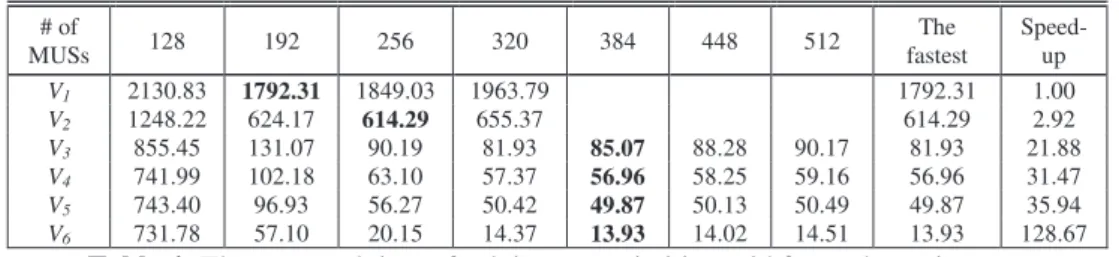
4.3 Overall Performances
By adding the computation time in Phase 1, the averaged computation time for each version is shown in Table 4. The original version, V1, took about 1792.31 seconds for each primitive grid. We estimate that it
would take about 311,000 years to check all 5,472,730,538 primitive grids to solve the minimum Sudoku problem. But the averaged computation time for V6 was greatly reduced to 13.93 seconds for each
primitive grid. Thus, we estimate that it would take only 2417 years on one core to solve the minimum Sudoku problem. The total speedup was about 128.67.
# of MUSs 128 192 256 320 384 448 512 The fastest Speed-up V1 2130.83 1792.31 1849.03 1963.79 1792.31 1.00 V2 1248.22 624.17 614.29 655.37 614.29 2.92 V3 855.45 131.07 90.19 81.93 85.07 88.28 90.17 81.93 21.88 V4 741.99 102.18 63.10 57.37 56.96 58.25 59.16 56.96 31.47 V5 743.40 96.93 56.27 50.42 49.87 50.13 50.49 49.87 35.94 V6 731.78 57.10 20.15 14.37 13.93 14.02 14.51 13.93 128.67
Table 4: The averaged time of solving one primitive grid for each version.
In order to have more confident in the result, we also randomly chose another set of 100 primitive grids and ran them again using V1 for 192 MUSs and with V6 for 384 MUSs, and the times for them were
1704.25 seconds and 10.99 seconds, respectively. The speedup was about 155.07, more than the above result, 128.67. Furthermore, we randomly chose another set of 10,000 primitive grids and ran them using V6 for 384 MUSs. For the 10,000 primitive grids, each was solved in about 12.72 seconds on average,
close to the above results for 100 grids. We did not try V1 or other versions since they would take a large
amount of time. The chosen primitive grids are also listed in the webpage of the Sudoku project (2010). 4.4 Different Sequences of Shrinks in the Improved DMUS Algorithm
For the improved DMUS algorithm described in Subsection 3.2, we may choose different sequences of Shrinks. In our experiments, we considered the following six sequences.
1. Perform Shrink(1) only.
2. Perform Shrink(1), Shrink(2), …, Shrink(r). 3. Perform Shrink(r), Shrink(r-1), …, Shrink(1).
4. Perform Shrink(1), Shrink(2), …, Shrink(r), Shrink(r-1), …, Shrink(1). 5. Perform the second sequence (above) twice.
6. Perform the second sequence (above) repeatedly until no more clues could be pruned.
Method 1 2 3 4 5 6
Average
Time (sec) 18.18 13.97 13.93 15.62 16.88 17.16 Table 5: The average solving times of using different sequences.
Table 5 shows the performances of version V6 using the above sequences, respectively. This result
indicates that the version performed best by using the second and third sequences, and that the third performed slightly better than the second. For version V4, we also obtained a similar result. Therefore, we
4.5 Node Counts in Phase 2
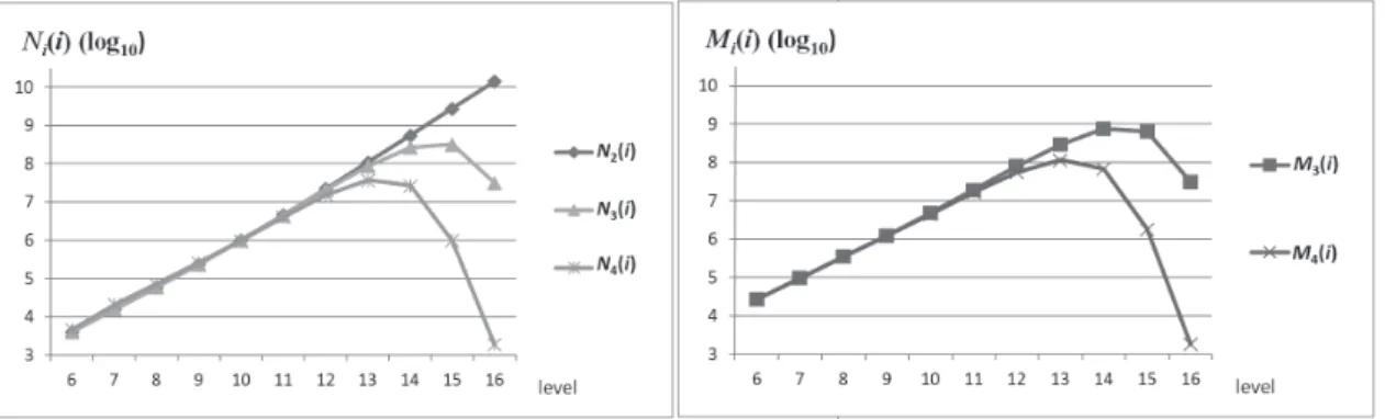
The key of the DMUS algorithm is to reduce greatly the number of nodes by paying the price of finding disjoint MUSs. This subsection investigates the number of visited nodes and the number of disjoint MUSs in Phase 2 in versions V2, V3, and V4. Let N2(i), N3(i), and N4(i) denote the total numbers of nodes
at level i of the search tree in V2, V3, and V4, respectively and M3(i) and M4(i) denote the total numbers of
disjoint MUSs generated from the nodes at level i of the search tree in both V3 and V4 respectively.
Figure 10 shows these numbers (in log10) at each level. For N2(i), it is clear that the maximum is at level
16 and is up to 14 billion. The maximum for N3(i) is shifted to level 15 and is up to 322 million, while the
maximum for M3(i) is to level 14 and is up to 745 million. Again, the maximum for both N4(i) and M4(i)
are shifted to level 13 and are up to 37 million and 115 million, respectively. This shows that the two DMUS algorithms are able to reduce the numbers of nodes at higher levels, which are normally enormous.
(a) (b) Figure 10: The numbers of (a) visited nodes and (b) disjoint MUSs.
Now we investigate the average number of disjoint MUSs generated from each node at level i, denoted by D3(i) in version V3. Figure 11 shows D3(i) and the ratio of D3(i)/(r+1) at each level i. From the figure,
the ratio is near 1 at levels 14 to 16. This also implies that it is highly likely to find more than r disjoint MUSs and therefore prune most of the subtrees rooted at levels 14 to 16. This explains why the DMUS algorithm performed well.
Figure 11 (a): D3(i) (b): the ratio D3(i)/(r+1).
Let us look into the value N3(i) more closely. Let Neq,3(i) denote the total number of nodes at level i,
which generate exactly r disjoint MUSs, and Ngt,3(i) denote the total number of nodes at level i, which
generate greater than r disjoint MUSs. Ngt,3(i) indicates that Ngt,3(i) nodes at level i can be pruned, and
Neq,3(i) indicates that Neq,3(i) nodes at level i may be further pruned by the improved DMUS algorithm.
Figure 12 indicates that the ratio of Neq,3(i) to N3(i) is significant at levels 7 to 14. This motivated the
Figure 12: Neq,3(i) and Ngt,3(i).
In version V4, we further separate the value Neq,4(i) into Neq,prune,4(i), Neq,shrink,4(i), and Neq,none,4(i).
Neq,prune,4(i) denotes the number of the Neq,4(i) nodes which can be all pruned by the improved DMUS
algorithm, as described in Subsection 3.2. Similarly, Neq,shrink,4(i) denotes the number of the Neq,4(i) nodes
which can be partially pruned, and Neq,none,4(i) denotes the number of the Neq,4(i) nodes which cannot be
pruned at all. Figure 13 shows a large portion for Neq,prune,4(i) and a very small portion for Neq,none,4(i) in
most Neq,4(i). This indicates that the improved DMUS algorithm is effective.
Figure 13: Neq,none,4(i), Neq,shrink,4(i), Neq,prune,4(i) and Ngt,4(i).
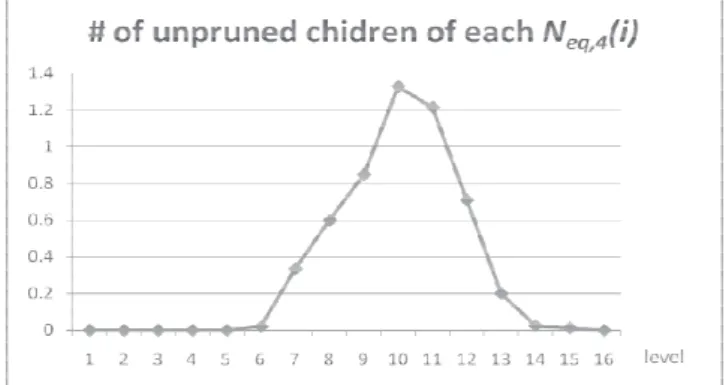
Figure 14 shows the average number of children generated from each of the Neq,4(i) nodes, which cannot
be pruned. In this figure, we observe that only the Neq,4(i) nodes at both levels 10 and 11 generated more
than one child on the average in the tree search, and the remainder generated less than one child on the average when using the improved DMUS algorithm. This shows that Neq,4(i) nodes do not generally grow
exponentially. This demonstrates the advantage of the improved DMUS in another aspect.
5. CONCLUSION
The contribution of this paper is to propose a new approach to solve the minimum Sudoku problem more efficiently. This paper presents a more efficient algorithm, named DMUS, incorporates it into the program CHECKER, and makes some more modifications including tuning the program to reduce greatly the computation times for finding n-clue puzzles from primitive grids.
According to our experiments, it took about 1792.31 seconds for the original CHECKER to solve one primitive grid on average. In contrast, our improved program presented above was able to solve one in 13.93 seconds on average. Thus, it is estimated that it takes only about 2417 years on one core to check all 5,472,730,538 primitive grids to solve the minimum Sudoku problem, while it would take the original about 311,000 years. If we had 10,000 cores, then we would solve it within three months, but it still takes more than 30 years when solved by the original CHECKER.
Using the modified program, it becomes more feasible to solve the problem on top of BOINC (Anderson, 2003). Thus, the authors of this paper were initiating a Sudoku project on top of the VTaiwan Project on BOINC (2010) to solve the minimum Sudoku problem by using the modified program.
ACKNOWLEDGEMENTS
The authors would like to thank the anonymous referees for their valuable comments, Hsin-Ti Tsai for helping some work in Phase 1, Gary McGuire for sharing his program CHECKER, Gordon Royle for sharing his 17-clue Sudoku puzzles, Glenn Fowler for sharing his program to generate 5.4 billion primitive grids, Horng-Liang Shih for helping to verify our program with 49151 17-clue puzzles, the National Center for High-performance Computing (NCHC) for computer time and facilities, Academia Sinica Grid Computing (ASGC) for computer time and facilities, Chunghwa Telecom for computer time and facilities of HiCloud, and the National Science Council of the Republic of China (Taiwan) for financial support of this research under contract number NSC 2221-E-009-102-MY3 and NSC 99-2221-E-009-104 -MY3.
6. REFERENCES
Anderson, D.P. (2003). Public Computing: Reconnecting People to Science, in Proceedings of the Conference on Shared Knowledge and the Web, November.
Anderson, D.P., Cobb, J., Korpela, E., Lebofsky, M., and Werthimer, D. (2002). SETI@home: An Experiment in Public-Resource Computing. Communications of the ACM, Vol. 45(11), pp. 56–61.
Berman, P., and Schnitger, G. (1989). On the Complexity of Approximating the Independent Set Problem, Springer-Verlag, Lecture Notes in Computer Science Vol. 349, pp. 256–267.
Delahaye, J.-P. (2006). The Science Behind Sudoku, Scientific American, Vol. 294(6), pp. 80–87. Felgenhauer, B., and Jarvis, F. (2006). Mathematics of Sudoku I, Math. Spectrum, Vol. 39, pp. 15–22. Fowler, G. (2007). Fowler's sudoku solver, http://www2.research.att.com/~gsf/sudoku/sudoku.html.
Huang, Y.-L. (2009). The Study of Minimum Sudoku, Master’s thesis (in Chinese), Graduate Department of Compute Science, National Chiao Tung University, Taiwan.
Lin, H.-H., and Wu, I.-C. (2010). Solving the Minimum Sudoku Problem, International Conference on Technologies and Applications of Artificial Intelligence (TAAI 2010), Hsinchu, Taiwan, November.
Mailer, G. (2008). A Guess-Free Sudoku Solver, Master’s thesis, Graduate Department of Computer Science, the University of Sheffield.
McGuire, G. (2006). Sudoku CHECKER and the minimum number of clues problem, http://www.math.ie/CHECKER.html.
McGuire, G., Tugemann, B., and Civario, G. (2012). There is no 16-Clue Sudoku: Solving the Sudoku Minimum Number of Clues Problem, http://www.math.ie/McGuire_V1.pdf, January.
Mersenne Research Inc. (1996). Great Internet Mersenne Prime Search – GIMPS, http://www.mersenne.org/prime.htm.
Palánek, R. (2011). Difficulty Rating of Sudoku Puzzles by a Computational Model, Proceedings of the 24th International FLAIRS Conference.
Royle, G. (2007). Minimum sudoku. http://people.csse.uwa.edu.au/gordon/sudokumin.php. Russell, E., and Jarvis, F. (2006). Mathematics of Sudoku II, Math. Spectrum, Vol. 39, pp. 54–58. Sudoku at VTaiwan Project on BOINC (2010). http://sudoku.nctu.edu.tw/, October.
Sudoku Forum (2009). http://www.setbb.com/phpbb/index.php?mforum=sudoku.
Sudoku Project on BOINC (2007). http://boincstats.com/stats/project_graph.php?pr=sudoku.
Wu, I-C., Chen, C.-P., Lin, P.-H., Huang, K.-C., Chen, L.-P., Sun, D.-J., Chan, Y.-C., and Tsou, H.-Y. (2009). A Volunteer-Computing-Based Grid Environment for Connect6 Applications, IEEE International Conference on Computational Science and Engineering (CSE-09), August 29–31, Vancouver, Canada.
Wu, I-C., and Lin, P.-H. (2010a). Relevance-Zone-Oriented Proof Search for Connect6, the IEEE Transactions on Computational Intelligence and AI in Games, Vol. 2(3), pp. 191–207.
Wu, I-C., Lin, H.-H., Lin, P.-H., Sun, D.-J., Chan, Y.-C., and Chen, B.-T. (2010b). Job-Level Proof-Number Search for Connect6. The International Conference on Computers and Games 2010 (CG2010), Kanazawa, Japan.
STOP PRESS
On January 1st, 2012, McGuire (McGuire et al., 2012) claimed to have solved the minimum Sudoku problem: No 16-clue puzzles exist. As their report claimed, they independently developed a new algorithm to solve this problem, started running jobs from January 2011 to December 2011, and took about 7.1 million core hours on the Stokes machine. In contrast, our preliminary version (Lin and Wu, 2010), submitted to TAAI 2010 in June 2010, started running jobs in October 2010. McGuire’s algorithm employed a method with higher-degree unavoidable sets, while our method used improved DMUS to prune subtrees. According to McGuire’s estimation (McGuire et al., 2012), the total computation time by their new algorithm is faster than that of ours by a factor of about 2. Further research is expected to investigate how to combine both techniques in the future and/or to apply them to some other similar problems, such as puzzle problems. Finally, the BOINC project (2010) will continue to solve this Sudoku problem, since it is still worthy to confirm the result.