使用故障區域辨識技術之多重故障矽診斷

國 立 交 通 大 學

電 子 工 程 學 系 電 子 研 究 所 碩 士 班

碩 士 論 文

使用故障區域辨識技術之多重故障矽診斷

Multiple-Fault Silicon Diagnosis Using Faulty

Region Identification

研 究 生 ： 蔡孟家

指 導 教 授 ： 周景揚 博士

使用故障區域辨識技術之多重故障矽診斷

Multiple-Fault Silicon Diagnosis Using Faulty

Region Identification

研 究 生：蔡孟家

Student: Meng-Jia Tsai

指導教授：周景揚 博士

Advisor: Dr. Jing-Yang Jou

國 立 交 通 大 學

電子工程學系 電子研究所碩士班

碩 士 論 文

A Thesis

Submitted to Department of Electronics Engineering & Institute

of Electronics College of Electrical and Computer Engineering

Institute of Electronics

National Chiao Tung University

in Partial Fulfillment of the Requirements

for the Degree of

Master of Science

in

Department of Electronics Engineering

August 2008

HsinChu, Taiwan, Republic of China

使用故障區域辨識技術之多重故障矽診斷

研究生：蔡孟家

指導教授：周景揚 博士

國立交通大學

電子工程學系 電子研究所碩士班

摘

要

Multiple-Fault Silicon Diagnosis Using Faulty

Region Identification

Student : Meng-Jia Tsai

Advisor : Dr. Jing-Yang Jou

Department of Electronics Engineering

Institute of Electronics

National Chiao Tung University

ABSTRACT

While designs are getting complex and technology becomes advanced, some errors may escape the verification flows pre-silicon, but exhibit on silicon. Because of physical limitation of chips, it is difficult to access data in chips. If errors occur, silicon diagnosis takes more and more time due to the limitation, especially for locating the fault sites. Thus many researches are developed for finding the fault locations. Targeting on multiple faults, we propose a diagnosis framework. In the framework, our algorithm can identify a region covering all faults then it removes impossible candidates. After the remaining candidates are ranked, real faults can be arranged to top of the list. We repair the first one and test the circuit again. With iterative diagnosis, repairing and testing, performance of our algorithm is enhanced. The experiment results show all fault sites can be identified in a few iterations with the proposed diagnosis framework.

Acknowledgement

I greatly appreciate my advisor, Professor Jing-Yang Jou, for his guidance, lead, and support during these two years. He provides many resources and creates an excellent environment for research. I am proud to be his student and a member of EDA Lab. I am also grateful to my co-guidance advisor, Professor Chia-Tso Chao, for his valuable suggestions. I am indebted to Meng-Chen Wu, Geeng-Wei Lee, and Che-Hua Shih for their discussion and help on my research. Without them, I cannot cross the barrier and bottleneck.

Specially thanks my partners, Yen-Yu Chen, Yang-Ting Mi, and Kuang-Wei Chen, for encouragement and friendship. And thanks Cheng-Yeh Wang, Zwei-Mei Lee, Bu-Ching Lin, and other friends in EE department and on net. They enrich my life not only in academic field but also society and entertainment. Chatting with them make me refreshed and released to confidently face the problem. Fi-nally, I would like to express my sincerely acknowledgements to my family who is always on my side, encouraging and patient of me.

Contents

摘要 . . . ii

Abstract . . . iii

Acknowledgement . . . iv

Contents . . . v

List of Tables . . . vii

List of Figures . . . viii

1 Introduction . . . 1

1.1 Previous Works . . . 3

1.2 Motivation . . . 5

2 Preliminaries . . . 7

2.1 Problem Formulation . . . 8

3 Faulty Region Identification & Ranking . . . 10

3.1 X-region . . . 11

3.2 Not Stuck-at-0 & Not Stuck-at-1 . . . 13

3.3 Faulty Region Identification . . . 15

3.3.1 Initial X-region Identification . . . 15

3.3.2 X-region Shrinking Algorithm . . . 19

3.4 Ranking . . . 32

4.1 Results for Single Fault . . . 38

4.2 Results for Multiple Faults Restricted in Length of Diameter of 2 40 4.3 Results for Multiple Faults without Diameter Restriction . . . 42

4.4 Results Using Proposed Diagnosis Framework . . . 45

5 Conclusions and Future Work . . . 48

References . . . 50

List of Tables

3.1 Patterns and responses . . . 16

4.1 Circuit parameters . . . 36

4.2 Results of diagnosis for single fault . . . 39

4.3 Results of multiple faults in length of diameter of 2 . . . 40

4.4 Comparison with [20] . . . 41

4.5 X-region shrinking of diagnosis for 3 faults . . . 42

4.6 Fault to the boundary & ranking of diagnosis for 3 faults . . . 43

4.7 X-region shrinking of diagnosis for 5 faults . . . 43

4.8 Fault to the boundary & ranking of diagnosis for 5 faults . . . 44

4.9 X-region shrinking of diagnosis for 8 faults . . . 44

4.10 Fault to the boundary & ranking of diagnosis for 8 faults . . . 45

4.11 Comparison between w/o and w/ the repair step for 3 faults . . . 46

4.12 Comparison between w/o and w/ the repair step for 5 faults . . . 46

List of Figures

2.1 Adaptive diagnosis framework . . . 7

2.2 Two categories of patterns . . . 8

2.3 Shrink the region to make faults close to the boundary . . . 9

3.1 Diagnosis illustration . . . 10

3.2 X-region . . . 11

3.3 The boundary of X-region . . . 12

3.4 Deduction stops at a gate whose signal is dominated by real fault 14 3.5 Flow of faulty region identification . . . 15

3.6 Fault assumptions, G1 stuck-at-1, net18 stuck-at-1 . . . 16

3.7 Active Fan-in for AND in [25] . . . 17

3.8 Active path tracing from erroneous output G16 . . . . 17

3.9 Fault simulation may be incorrect if not all real faults covered in the X-region . . . 18

3.10 The initial X-region in the example . . . 19

3.11 Example of algebra of 3-value simulation . . . 20

3.12 X-region shrinking algorithm . . . 20

3.13 Apply pattern (G1, G2, G3, G4, G5) = (11010) for logic simulation 21 3.14 Force values in the X-region to X . . . . 21

3.16 Flipping & mismatch . . . 23

3.17 Flip net14 at pattern (G1, G2, G3, G4, G5) = (11010) . . . . 25

3.18 Remove net14 from the X-region . . . 26

3.19 It cannot identify more good values at pattern (10101) . . . 27

3.20 Identify good values using input information . . . 28

3.21 Is Input Good(tg, p) . . . 30

3.22 Identification using input values . . . 31

3.23 The auxiliary value helps another identification . . . 31

3.24 Candidates are divided into 2 groups . . . 33

3.25 Full-match candidates are divided into 3 groups . . . 34

3.26 Illustration of sorted candidate list . . . 35

4.1 Fault injection . . . 37

4.2 Example for diameter . . . 37

Chapter 1

Introduction

Pre-silicon verification, such as formal verification and stimulus generation, aims to verify functions of designs and fixes design errors before manufacturing. However, due to the increasing design complexity, some errors cannot be predicted and detected in pre-silicon verification flow. They only exhibit on chips [1]. The process, silicon diagnosis, is utilized to identify the reasons of errors on chips and feeds the information back to engineers. By silicon diagnosis, engineers can fix the fault sites or modify the design to prevent the same errors on later manufactured chips. Unfortunately, the time of silicon diagnosis takes grow rapidly because of increasing circuit complexity, limited controllable and observable pins on a chip, limited storage resources on automated-test-equipment(ATE) and many types of faults on a chip. Silicon diagnosis becomes the most time-consuming step, even more than 35% of time-to-market [1] up to 50% nowadays [2], and the most costly step than other aspects of manufacturing [3]. Therefore, an effective silicon diagnosis methodology is needed to accelerate the process and reduce time-to-market.

The major part in silicon diagnosis is fault localization [1]. The objective of fault location is to indicate systematic errors and to pinpoint the root-cause of the errors. Conventionally, there are two categories of diagnosis algorithm: cause-effect and cause-effect-cause. In cause-cause-effect algorithm, defects are modeled to logic-level behavior and simulated with fault simulator to catch the fault syndrome beforehand. The fault syndromes are stored in the fault dictionary. Once errors are observed during testing, engineers can search the fault dictionary to find the matched response and obtain the fault sites quickly. But the dictionary becomes large due to the increasing design complexity and needs much storage to save even

the dictionary compressed. It also needs to consider the combinations of multiple faults which make the dictionary larger. On the contrary, effect-cause algorithm locates fault sites without building the fault dictionary. It analyzes test responses and deduces from erroneous outputs. It determines fault candidates whose signals probably propagate to the erroneous outputs. Usually fault simulation is used to validate the deduction. This kind of algorithm is memory-efficient for high complexity designs.

Fault models are explicitly or implicitly [4,5] utilized in these two categories of diagnosis algorithms, especially in the fault simulation step, to make quality of diagnosis more accurate. Fault modelling usually abstracts the defect behavior to logical behavior. Stuck-at fault is the simple and static fault which is widely used [6,7]. For example, single stuck-at fault is used for test-pattern generation and all commercial tools have been built functions for the fault model. However, it is too restricted and unrealistic because defects may occur at multiple locations and are unconstant for different patterns. Some faults may not be detected with patterns generated for single stuck-at fault and more than 41% defects cannot be diagnosed with single stuck-at fault [5]. For detection, n-detection technique can be used with single stuck-at fault model to enhance the probability of detecting faults. In [8], 5-detection technique increases the probability of detection from 75% to 99% on bridge fault without additionally complex fault models. For diagnosis, an alternative approach to enhance single stuck-at fault is multiple stuck-at fault model. Several faults such as bridge fault [9,10], transition fault [5,11], and open-interconnect fault [12] can be transformed to multiple stuck-at faults and diagnosed indirectly. It preserves the concision of stuck-at fault and accurately represents real defects than single stuck-at fault model. For multiple stuck-at fault model, existing fault simulator can be employed with only a little modification. Hence, there are many researches for diagnosing multiple stuck-at faults [13–17]. Other researches for multiple-fault diagnosis can also be applied for locating multiple stuck-at faults [6,12,18–22].

1.1

Previous Works

Region-based technique [18–20] assumes that faults locate in a user-specified region. The distance is the minimum number of wires needed to traverse from a fault to the center [18]. Distance between faults and the center of region must be less than a specified radius. Region-based technique forces output values of the region to unknown in simulation. The target region probably contains real faults and its unknown signals may propagate to erroneous outputs. All sites in the circuit have to be center of regions for examination. Thus region-based technique needs to simulate many times to identify the candidate regions. However, we do not know the length of radius in reality. If it begins from radius 1, as the radius becomes larger, time of diagnosis grows exponentially in the experimental results of [18]. In [23], faults may occur nearby. A realistic algorithm is still needed for this problem. Unknown model is first proposed in [4]. It considers faulty signals in simulation to be unknown instead of accurately modeling the behavior. Thus it is suitable for complex defects. It is also utilized in [6,12] without a specified region. In [12], it selects initial candidates using path-trace counts with unknown model then prunes impossible ones and validates with 3-value simulation for open-interconnect problem. In [6], it also simulates single-unknown candidate under single-location-at-a-time(SLAT) assumption and calculates scores of candidates for Byzantine faults.

SLAT-based algorithms are popular in diagnosis [6,17,23–25] recent years. In [5], SLAT properties are completely explained. SLAT-based algorithms assume that faulty signals converge on one site even multiple defects existing and only considers fault location rather than fault behavior. The condition of faulty signals converging on one site is equivalent to activate a fault site and explains the faulty syndrome at a failing pattern. Therefore, it only selects failing patterns which have SLAT properties to analyze. The fault sites which explain more SLAT patterns are more possible in real fault sets, and the possible fault sets are combinations of different fault sites which explain all failing patterns.

SLAT-based algorithms are efficient because there is only single fault at each failing pattern. Besides, SLAT-based algorithms are model independent because they do not consider fault behavior and root-cause of each SLAT pattern can be unrelated. However, SLAT-based algorithms do not mention how to identify the fault sites if they are far from the convergent point. It is difficult to diagnose with SLAT if there are multiple faulty signals diverged, masked or interacting to cancel fault effects [17].

In [6,18,22,23,25], the ranking approach is utilized. While there are too many candidates and candidates cannot be tried entirely, it should start verifying from the most possible one. Candidates are sorted with scores and usually the higher ones of the candidate list are arranged former. No candidate will be eliminated during the procedure to prevent wrong elimination with heuristic determination. The worst case is that all candidates need to be tried to obtained all faults. In these papers, the ranking approach formulates scores with matching criterion. Generally a match is that values on one output pin from simulation and test response are the same, whereas a mismatch is the values in different status. Scores at a pattern are functions of numbers of matches and mismatches. The partial match, a portion of scores, is that the value on one output pin from simulation is unknown [18]. In [25], it divides mismatch into two parts, not-explained and mis-predict signals. Not-explained signals are signals correct at test responses while simulation responses incorrect. In contrast, mis-predict signals are signals incorrect at test responses while simulation responses correct. In [22], an input vector is curable if simulation responses are all consistent with test responses while pseudo faults are injected. The curable-vectors are considered more important than other patterns so that the candidates causing the vectors are sorted prior to others. Structural relationship is considered in [6]. Candidates far from outputs are are more potential than near ones.

After fault sites are identified, the design needs to be modified and re-spin to prevent errors occur in next production. But mask-cost grows exponentially

as technology being advanced. Large percent of expense is for active devices [26]. Thus placing Design-for-Debugging(DfD) components on chip, such as spare cells, makes chips be repaired with focused-ion-beam(FIB) or engineering-change-order(ECO). They modified metal layers or mask of metal layers without rewriting a new one to reduce the expense [27]. Although chips may be oxidized due to package uncovered, the success probability is acceptable.

1.2

Motivation

In reality, we do not know the distance among faults, hence we cannot assume a limited region covering all faults which is proposed in the research of region-based model [18,20]. For the limited storage of automated test equipment(ATE), a small set of patterns is usually generated for fault detection. One pattern may activate as many fault sites as possible at the same time. Many faulty signals are excited while many faults exist. While faults are close to each other, there can be many patterns causing faulty signals to cancel each other on some primary outputs [17]. Multiple faults activated simultaneously or close to each other are difficult to be diagnosed with SLAT-based algorithm.

In this thesis, we target on multiple stuck-at faults on gates in gate-level circuits. We do not assume number of faults and the distance among faults in our methodology. Our idea is to find a region covering all faults even they are masked or their effects can be cancelled. Then we do not identify the faults directly. We remove the impossible candidates to prune the size of candidates. During the pruning, we must guarantee real faults are not removed. Therefore, we can find faults in the region. To verify that we obtain the real faults, we can repair the most possible candidate and test the circuit again. If there is still any error, we have to try another site in the reported region. However, the responses also provide information about fault locations. Combining with repairing and testing information each iteration, we can adaptively find all faults.

The rest of the thesis is organized as follows. Chapter 2 introduces the proposed diagnosis framework, the assumptions and objective for our problem. In Chapter 3, the proposed algorithms, faulty region identification and ranking, are explained. The experimental results are shown in Chapter 4. Finally, Chapter 5 concludes the thesis.

Chapter 2

Preliminaries

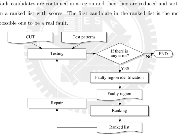
We propose the adaptive diagnosis framework shown in Figure 2.1. Given a circuit-under-test(CUT) and test patterns, we can obtain the test responses from ATE in testing step. If any error at primary outputs is obtained, there must be faults detected. The following procedure is our algorithm, faulty region identification and ranking, to find where is the root-cause. In these two steps, all fault candidates are contained in a region and then they are reduced and sorted in a ranked list with scores. The first candidate in the ranked list is the most possible one to be a real fault.

Figure 2.1: Adaptive diagnosis framework

We fix the first one and do testing again. A different set of response could be obtained if a fault is repaired. The procedure is run until there is no error obtained at primary outputs and scan dumps.

2.1

Problem Formulation

In this thesis we assume the circuit is a full-scan and verified one. In the full-scan scheme, all register are controllable and observable and the scan-chains are assumed fault-free. Test patterns can be shifted in and the responses are captured at next cycle. Behaviors of a sequential circuit are the same as a com-binational circuit in test mode. Pseudo primary inputs(PPI) and outputs(PPO) which are the outputs and inputs of registers can be regarded the same as primary inputs(PI) and outputs(PO). While we mention the primary inputs and outputs in this article, they are also combined with PPIs and PPOs. Subsequently, it is exhaustively verified before fabrication. Given a set of test patterns, if there is any error obtained in testing, there must be some faults on silicon to cause the syndrome. We assume the syndrome can be reproduced while applying the same patterns again. Erroneous outputs(EPO) are output pins whose signals are inconsistent in testing and logic simulation. Failing patterns are patterns in the test set which detect the faults and some outputs are EPOs. Passing patterns are the other patterns in the test set and all of the responses are consistent in testing and logic simulation. An example is shown in Figure 2.2.

(a) Failing pattern (b) Passing pattern

Figure 2.2: Two categories of patterns

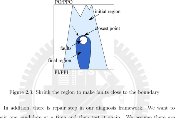
Given a circuit, test patterns and test responses, we can check if there are errors, then apply the proposed diagnosis algorithm to find the root-cause of errors. The algorithm reports a region covering all faults and candidates in the region are sorted in a ranked list. In the algorithm we remove the impossible

candidates from the region. The objective is to make real faults very close to the boundary of region and to the top of the ranked list. Thus we can obtain one of the faults closest to the boundary by utilizing structural information. The illustration is shown in Figure 2.3. We can also obtain the first fault in the ranked list in a few trials according to the order of the list.

Figure 2.3: Shrink the region to make faults close to the boundary

In addition, there is repair step in our diagnosis framework. We want to repair one candidate at a time and then test it again. We assume there are Design-for-Debugging(DfD) components built in the circuit such as spare cells. Applying the existing repair techniques causes only small side effects that can be ignored. If one fault is repaired, the test responses may be different from previous ones. Therefore, we can identify the fault sites and fix them adaptively.

Chapter 3

Faulty Region Identification &

Ranking

In this chapter, we describe the details in faulty region identification and ranking which are two parts of our proposed framework. The other steps are referred to other researches. There are three concepts used in faulty region iden-tification: X-region, not stuck-at-0 & not stuck-at-1 properties, and the X-region

shrinking algorithm. We define the first two and then describe the X-region

shrinking algorithm which is integrated in the flow of faulty region identification. The last is ranking.

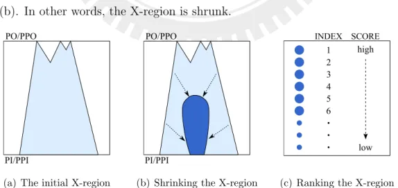
At beginning of faulty region identification, we identify an initial fault can-didate set, X-region, and the cancan-didates are gates. The illustration is shown in Figure 3.1(a). If we can guarantee a fault candidate is fault-free, the candidate is impossible to be a real fault and can be removed from the candidate set. Thus the size of candidate set is decreased with the elimination as illustrated in Figure 3.1(b). In other words, the X-region is shrunk.

(a) The initial X-region (b) Shrinking the X-region (c) Ranking the X-region

To remove fault-free candidates, we use the X-region shrinking algorithm to identify candidates with the not stuck-at-0 and not stuck-at-1 properties in the X-region described in section 3.2. A candidate with one of the properties helps the algorithm identify another fault and candidates with both two properties can be removed. Hence it iteratively decreases the size of X-region without losing real faults. Correctness of the identification is proved in later section.

After shrinking the X-region, impossible faults do not exist in the X-region. Finding real faults in this compact region is easier than the initial one. Finally, we rank the remaining candidates in the X-region to figure out the most possible fault site. It is shown in Figure 3.1(c). The closer faults located to the boundary, the easier they can be caught.

3.1

X-region

The X-region is a candidate set which contains all real faults. It is the substance operated by our algorithm and obtained in the first step described in section 3.3.1. Gates outside of the X-region are fault-free. The boundary is the edge between inside and outside of the region. The illustration of the X-region is shown in Figure 3.2.

Figure 3.2: X-region

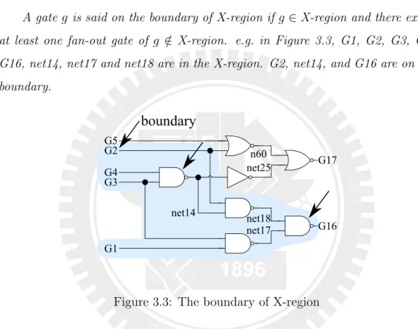
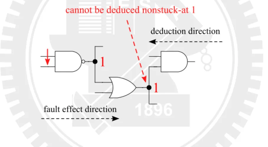
to primary outputs. In other words, obtaining faulty signals on boundary gates means they are on the error propagation paths of activated faults. Faults can be either on the boundary or inside the X-region. In our algorithm, we deduce the correctness of gates from the boundary to the inside of X-region. The definition of the boundary is as follows.

Definition 3.1. (The boundary of X-region)

A gate g is said on the boundary of X-region if g∈ X-region and there exists at least one fan-out gate of g /∈ X-region. e.g. in Figure 3.3, G1, G2, G3, G4, G16, net14, net17 and net18 are in the X-region. G2, net14, and G16 are on the boundary.

Figure 3.3: The boundary of X-region

Signals propagating through fault sites are replaced with faulty signals and input values of the faults is unknown. Under multiple-fault assumption, fault masking may occur and one faulty signal in the fan-in cone of another fault could also be replaced. We do not know the locations of masked faults but only know these faults may be inside the fan-in cone of the masking faults. For this reason, unless we know a gate g is fault-free, we cannot distinguish whether the fan-in gates of g is faulty or not. To detect faulty signal of g, we must make sure that there is at least one signal propagation path from it to primary outputs that all gates on the path are fault-free. Then we probably observe the effect from g. Gates on the boundary are guaranteed to have at least one fault-free fan-out. So

we only operate gates on the boundary in the algorithm. The deduction stops when non-masked real faults are on the boundary in ideal cases. The masked faults are still in the X-region without losing, but they cannot be accurately identified.

In our algorithm, we use single-fault simulation to identify fault-free gates on the boundary. Single-fault simulation is simple and widely used. In [5], there are some situations that multiple defects behave like a single fault and can be dealt with fault simulation. However, in multiple-fault-effect cases, single-fault simulation may misdiagnose. It cannot accurately describe multiple-single-fault behavior. To overcome this, all values of all gates in the X-region are forced to be unknown value during our algorithm. The unknown model used in [4,6,12,18– 20,28,29] is setting gate values to unknown. They determine fault candidates by observing if the unknown signals propagate to erroneous outputs in fault simulation. The unknown model enhances single-fault simulation then we can analyze one candidate at a time. If we inject a fault in the X-region and observe an error at primary outputs in simulation, we can claim the error is from the injected fault even under multiple fault condition. The algorithm is in section 3.3.2.

3.2

Not Stuck-at-0 & Not Stuck-at-1

Conventional stuck-at fault model is widely used. In the model, there is one of three states: stuck-at-0, stuck-at-1, or fault-free on a gate. But in our algorithm, we import the concept of not stuck-at-0 and not stuck-at-1 properties. If a candidate can be demonstrated that its signal is 0 on chip for a given pattern, the candidate should not be at-1. On the other hand, it should not be stuck-at-0 if its signal is guaranteed 1 on chip. A candidate is claimed fault-free if it is both not stuck-at-0 and not stuck-at-1 [15,16]. For convenience, we use NSA0 and NSA1 to represent not stuck-at-0 and not stuck-at-1, respectively. For not

specifying either 0 or 1, we use v to represent the value and NSAv to represent

not stuck-at-v.

In our algorithm, we want to remove fault-free candidates from the X-region by identifying they are NSA0 or NSA1. A candidate which is both NSA0 and

NSA1 can be removed. Real faults are at most determined one of these two faults.

The other value of these two fault cannot be determined because it is the same as the faulty value. Hence it is guaranteed that real faults must not be removed with the identification. We apply fault simulation in our algorithm to identify whether a candidate is fault-free. A NSA0 or NSA1 candidate is not necessarily identified in every patterns. Because stuck-at fault is a kind of static fault [6] and fault effect occurs while it is activated without special pattern dependency. An identified NSAv candidate at one pattern is sufficient to explain it is NSAv.

Figure 3.4: Deduction stops at a gate whose signal is dominated by real fault

We apply the X-region shrinking algorithm on the X-region boundary first and the inputs of the boundary to deduce NSA0 and NSA1 properties. For ideal case, the operation stops at the time that real faults are deduced. Unfortunately, some faults and their signal-dominated fan-outs are considered fault-equivalent [11]. The deduction stops at fault-equivalent gates before touching real faults. Figure 3.4 shows this situation. It remains redundant fault candidates. We will measure how far from real faults to the boundary in chapter 4.

3.3

Faulty Region Identification

Without number and distance assumptions of faults, we only conservatively identify a region containing all real faults. After finding the region, we can then easily catch real faults in it with structural information. The flow of our algorithm is shown in Figure 3.5.

Figure 3.5: Flow of faulty region identification

In this thesis, we utilize the example to describe how the X-region is shrunk with the algorithm shown in Figure 3.6. Assume there are two fault in the circuit,

G1 stuck-at-1 and net18 stuck-at-1. The test patterns, simulation responses and

test responses are shown in Table 3.1.

3.3.1

Initial X-region Identification

At the beginning of our algorithm, initial candidates are identified to form the initial X-region. Candidates are gates which are probably real faults detected

Figure 3.6: Fault assumptions, G1 stuck-at-1, net18 stuck-at-1

Test Pats. Sim. Resp. Test Resp. Failing PO G1 G2 G3 G4 G5 G16 G17 G16 G17 11010 11 01 G16 11001 11 01 G16 11011 11 01 G16 10001 01 01 – 01111 00 10 G16 00010 00 00 – 10101 11 11 – 00110 00 10 G16

Table 3.1: Patterns and responses

by a given test set. With lack of number and distance information of faults, we only know that faulty signals propagate to primary outputs. Thus we can back-trace from erroneous outputs to obtain fault candidates.

In [30,31], if an EPO z is observed, the circuit contains a fault in the fan-in cone of z. For one gate, not all inputs with faulty signals may change the output. It is sufficient to cover all real faults by tracing the sensitive inputs of a gate depending on test patterns. Some publications are based on critical path tracing [12,32–34]. It traces the only one controlling input pin or all non-controlling input pins of a gate. Otherwise, it stops tracing. It is suitable for single-fault diagnosis, however, it may lose faults in multiple-fault diagnosis. Two or more controlling pins of one gate may be inverted simultaneously due to multiple faulty signals. It should consider this situation to prevent losing real faults.

a b x Active Fan-in 0 0 0 a, b

0 1 0 a

1 0 0 b

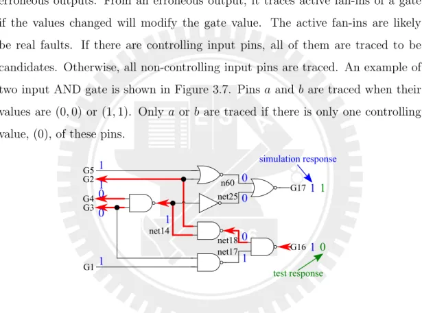
1 1 1 a, b Figure 3.7: Active Fan-in for AND in [25]

In [25], active path tracing is used to identify candidates which can effect erroneous outputs. From an erroneous output, it traces active fan-ins of a gate if the values changed will modify the gate value. The active fan-ins are likely be real faults. If there are controlling input pins, all of them are traced to be candidates. Otherwise, all non-controlling input pins are traced. An example of two input AND gate is shown in Figure 3.7. Pins a and b are traced when their values are (0, 0) or (1, 1). Only a or b are traced if there is only one controlling value, (0), of these pins.

Figure 3.8: Active path tracing from erroneous output G16

An example for tracing from erroneous outputs with active path tracing is shown in Figure 3.8. Comparing simulation and testing response, the primary output of G16 is erroneous. The bold connection lines are the traced paths. After tracing from the erroneous output, G16, net18, net14, and the primary inputs

G2, G3, G4 are candidates.

The X-region has to cover all real faults. However, tracing from one erro-neous output at a pattern may cover only part of real faults. Traced gates at

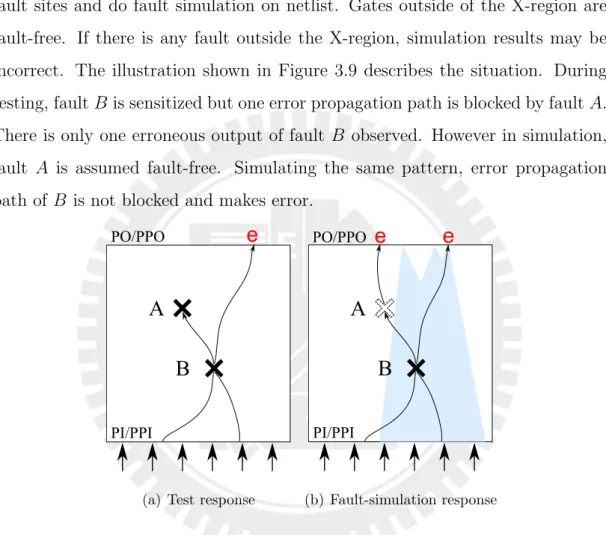
different patterns may cover different parts of faults. We then unite all traced gates to ensure all real faults are covered. In addition, it also covers masked faults. Although it is conservative that the initial X-region becomes large due to many erroneous outputs, uniting all traced gates is necessary for later step in the algorithm. With only test vectors and test responses, we can only assume fault sites and do fault simulation on netlist. Gates outside of the X-region are fault-free. If there is any fault outside the X-region, simulation results may be incorrect. The illustration shown in Figure 3.9 describes the situation. During testing, fault B is sensitized but one error propagation path is blocked by fault A. There is only one erroneous output of fault B observed. However in simulation, fault A is assumed fault-free. Simulating the same pattern, error propagation path of B is not blocked and makes error.

(a) Test response (b) Fault-simulation response

Figure 3.9: Fault simulation may be incorrect if not all real faults covered in the X-region

In the example shown in Figure 3.10, it traces G1, G2, G3, G4, net14, net17,

net18, and G16 to form the initial X-region. The boundary consists of G2, net14,

Figure 3.10: The initial X-region in the example

3.3.2

X-region Shrinking Algorithm

The X-region shrinking algorithm is applied to identify candidates which are not faulty. It is similar to [20] which distinguishes impossible faulty regions from possible ones to improve the original region-based methodology in [18]. We propose a different the X-region shrinking algorithm to find gates belonging to the X-region are NSA0 and NSA1. It focuses on one target gate at a time with respect to one pattern to verify if the target gate has good value on chip which means it is consistent with simulated value. A target gate which is guaranteed to have good value v on chip indicates that it is NSAv. The target gate is fault-free and can be removed from the X-region if it is determined to be both NSA0 and

NSA1.

NSA0 and NSA1 deduction is based on fault simulation technique. It utilizes

all patterns, including failing patterns and passing patterns. Under multiple fault assumption, conventional single-fault simulation may misdiagnose, especially on the condition that fault effects interact with each other. The interaction may change faulty signals to good signals, but single fault simulation cannot reflect the interaction. We apply 3-value simulation on the X-region in the X-region shrinking algorithm to avoid misdiagnosing and losing real faults. The algebra of 3-value simulation for each gate is from [35]. Assuming there are unknown input signals, the gate value can be determined if there are controlling input signals.

Otherwise, the gate value is unknown. An example is shown in Figure 3.11.

(a) Controlling signal exists (b) No controlling signal

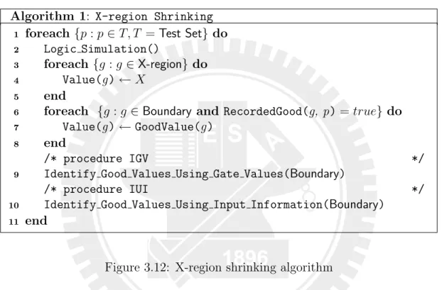
Figure 3.11: Example of algebra of 3-value simulation Algorithm 1: X-region Shrinking

foreach {p : p ∈ T, T = Test Set} do

1 Logic Simulation() 2 foreach {g : g ∈ X-region} do 3 Value(g )← X 4 end 5

foreach {g : g ∈ Boundary and RecordedGood(g, p) = true} do

6 Value(g )← GoodValue(g) 7 end 8 /* procedure IGV */

Identify Good Values Using Gate Values(Boundary)

9

/* procedure IUI */

Identify Good Values Using Input Information(Boundary)

10

end

11

Figure 3.12: X-region shrinking algorithm

The region shrinking algorithm is shown in Figure 3.12. The initial X-region is obtained with active path tracing. For each pattern, we do logic simula-tion at line 2 to initialize simulated values on all gates. Gate values belonging to the X-region are forced to be unknown values at line 3 and on-boundary ones are reloaded recorded good values to initialize the X-region at line 6 if the values are identified in later functions. Subsequently, it utilizes gate values to identify good values and NSA0, NSA1 properties at line 9. If NSA0 and NSA1 properties on a target gate are identified, the procedure at line 9 remove the target gate from the X-region. To further identify more good values, we deduce the input values of a target gate at line 10. The procedure at line 10 helps previous identification to remove more candidates from the X-region.

As shown in Figure 3.13 and Figure 3.14, the circuit is applied a pattern for logic simulation to get simulated values for all gates. Then gates in the X-region are forced to be value X which is the unknown symbol in simulation.

Figure 3.13: Apply pattern (G1, G2, G3, G4, G5) = (11010) for logic simulation

Figure 3.14: Force values in the X-region to X

Following X-region initialization is procedure IGV, Identify Good Values Using Gate Values at line 9 in Figure 3.12, and the detail is shown in Figure 3.15. We randomly choose a target gate on the boundary with unknown value and force its value to be the reverse of the simulated value. This is the flipping step at line 2. The reverse value is a pseudo-faulty signal injected in the circuit. All forced values are unchangeable during simulation. After 3-value simulation at line 3 is conducted, if there is mismatch defined in Definition 3.2 at a primary output comparing with test response, the value on target gate must be consistent with simulated value and cannot stick at the reverse value. So that the target gate has a good value and one of NSA0 and NSA1 properties. As shown in Figure

Procedure IGV: Identify Good Values Using Gate Values(Boundary) foreach {g : g ∈ Boundary and Value(g) = X} do

1

Flip(g)

2

3-Value Simulation()

3

foreach {z : z ∈ P O, P O = Primary Output} do

4

if Mismatch(z) then

5

if NSAValue(g) = GoodValue(g) then

6

X-region← X-region − {g}

7

Boundary ← Boundary ∪ {F Ig : F Ig ⊆ FanIn(g)andFIg ⊂

8 X-region} else 9 RecordedGood(g, p)← true 10 NSAValue(g )← GoodValue(g)0 11 end 12 break 13 end 14 end 15 end 16

Figure 3.15: Identify good values using gate values

3.16, G17 has a mismatch and G2 must have good value 1. In other words, G2 is NSA0. Therefore, procedure IGV utilizes gate-value flipping to identify NSA0 and NSA1 properties. If both NSA0 and NSA1 properties are identified on the target gate, the target gate can be removed from the X-region at line 7.

Definition 3.2. (Mismatch between 3-value simulation and test response)

Mismatch between 3-value simulation and test response at one primary output is that the output pin has 0,1 values and are different between 3-value simulation and test response, e.g. in Figure 3.16, we flip G2 from 1 to 0 and G17 gets a mismatch because G17 has 1 in test response but 0 in 3-value simulation after 3-value simulation. G2 must have good value 1 and be NSA0.

The target gate actually with good value v is NSAv0. We will force its value to be good one for next target gate at the same pattern. If simulation results are unknown or consistent with passing outputs, the target gate may be not activated or the effect does not propagates to primary outputs. Even erroneous outputs

Figure 3.16: Flipping & mismatch

from simulation match real erroneous outputs, we do not know what situation the target gate is. It can be either a stuck-at fault or just on the error propagation paths from a combination of real faults inside the X-region. We can only judge the correctness with mismatch. If there is no mismatch observed at primary outputs, the situation of target gate is still unknown. The proof is below.

Theorem 3.3. Given an X-region, there is a set of gates on the boundary(BG).

For one pattern, assume there is a set of gates on the boundary whose val-ues are forced to be good valval-ues(BGF G), and a set of gates are forced to be unknown(BGF U ). BGF G is a subset of BG, BGF G ⊂ BG, and its size is larger or equal to 0, |BGF G| ≥ 0. BGF U contains gates in BG except in BGF G, BGF U = BG− BGF G. Flipping a gate g, g ∈ BGF U, and simulating, if there is any mismatch observed at primary outputs, g must have good value the same as simulated one and should be in BGF G.

Proof. At the same pattern,

1. All gates in BG have unknown values, BG = BGF U . An arbitrary gate

g, g ∈ BGF U, is set to v0 which is reverse of simulated value v. If any mismatch is observed at outputs, g must have good value v consistent with simulated one. That is to say g is NSAv0 and g ∈ BGF G. g is forced to be good value on the boundary for next target gate at the pattern.

It is obviously established. Gates in BG are unknown except g. The in-consistent signal must originate from g. Setting good value on g is the only way to eliminate the inconsistency.

2. Following procedure IGV, assume there are k gates on the boundary forced to be good values, |BGF G| = k, and it is valid to set these gates to good values.

3. Subsequently, we randomly choose the (k + 1)th gate in BGF U . If flipping the (k + 1)th value causes mismatch, the (k + 1)th gate must have good value at current pattern.

Supposing setting the (k + 1)th to good value is not valid, there must be any invalid assignment in previous k gates in BGF G. If i, 1≤ i < k, is the invalid assignment, there must exist j, 1 ≤ j < i, invalid. By the recursive relationship, it is deduced that the first assignment is invalid. It contradicts the first assignment. However, first condition is obviously established. The (k + 1)th assignment must be valid.

By mathematical induction, if there are n gates in BG forced to be good values and the others are unknown, the (n + 1)th value is good while mismatch is observed after 3-value simulation.

Theorem 3.3 is for the same pattern. Given another pattern, all statuses on the boundary have to be reset to unknown or recorded values at the new pattern. Gate values are set to unknown for two reasons. One reason is that good values on gates may be different due to a new pattern. The other reason is that even the boundary gate is NSAv0 and recorded at previous patterns, we do not know in reality it has good value v at current pattern. There are still two cases on the boundary gate, stuck-at-v or fault-free, causing different values on the boundary gate. If it sticks at good value v, obviously the value is good value and the pattern does not activate the fault. If it is fault-free, the value depends on values of its fan-ins. It gets good value v if there is no faulty signals in its fan-in cone. On

the other hand, it may get faulty value v0 which is reverse of good value if it is on the error propagation paths of some faults inside its fan-in cone. Setting good value on it by inheriting the recorded value from previous patterns may make a mistake. Because of these reasons we need to reset the status to unknown and do the identification again to check.

Nevertheless there is one exception. Boundary gates on primary inputs can be set to good values while the value is recorded in previous patterns. Because we assume that there are no errors on scan-chains, all values fed in primary inputs are good values. Both two cases, stuck-at-v or fault-free, are guaranteed that the pins have good values, they can be set to good values and skip procedure IGV.

Figure 3.17: Flip net14 at pattern (G1, G2, G3, G4, G5) = (11010)

As shown in Figure 3.17, G2 is forced to be good value and then next target

net14 is flipped to 0 at the same pattern. The mismatch occurs which means that net14 must have good value 1 and be NSA0. At another pattern, net14 is chosen

to be the target and flipped to 1. It also makes an mismatch which shows net14 must have good value 0 and be NSA1. Therefore, net14 is NSA0 and NSA1 and it can be removed from the X-region. G3, G4 are new members of the boundary shown in Figure 3.18.

In summary, procedure IGV shown in Figure 3.15 utilizes gate-value flipping to identify good values. Targets on the boundary can be removed from the X-region if NSA0 and NSA1 properties are identified. Gates in the X-X-region have

(a) net14 is NSA1 at Pattern (G1, G2, G3, G4, G5) = (01111)

(b) Update the X-region & boundary

Figure 3.18: Remove net14 from the X-region

unknown values except gates on the boundary with good values identified. In procedure IGV, the condition of observing mismatch is that a pseudo-faulty signal must propagate through fault-free gates to primary outputs without blocking by unknown signals after 3-value simulation. However, we flip one value on the boundary one time and keep the others unknown if they have no identified good value. Pseudo-faulty signals, especially non-controlling values or gates with only one fault-free fan-out, are easily blocked by the other signals. The excep-tions are controlling signals whose computation priority in 3-value simulation is higher than unknown. The controlling values dominate gate-output signals. Some boundary gates are recorded not stuck-at controlling values because pseudo-faulty signals are controlling signals in the process of flipping. But we cannot get not stuck-at non-controlling ones even if it actually is fault-free. If no mismatch is observed, no good value is identified. That is the reason that the X-region cannot

be shrunk anymore.

In the example after procedure IGV, G1, net17, net18 remain in the X-region and net17, net18 are NSA0. net17 is actually fault-free but it cannot identify

net17 NSA1 shown in Figure 3.19. The signal can be blocked by the unknown

value of net18.

(a) (b)

Figure 3.19: It cannot identify more good values at pattern (10101)

But without the X-region, the pseudo-faulty signal may propagate to primary outputs to make mismatch. That is to say while the other gates on the boundary have good values, the pseudo-faulty signal from the flipping step may propagate to primary outputs to make mismatch. After a good value is identified in procedure IGV, we force the target gate to be good value for next identification in the same pattern. It helps next pseudo-faulty signal propagate to primary outputs. For this reason, if more good values can be identified, more NSA0 and NSA1 properties can be identified and the X-region can also be shrunk further.

Some situations can be analyzed more and solved. We propose procedure IUI, Identify Good Value Using Input Information at line 10 of X-region shrinking algorithm in Figure 3.12, based on the flipping and mismatch concept using input signals of target gates to further identify more good values. We still randomly choose a target gate on the boundary with unknown value and then we deduce the input values of the target gate. Assuming simulated value of the target gate is v at a pattern, if it is NSAv0 and its input values are good, it must have good value v. Thus, to verify the target gate with good value v, it needs any of input pins with identified controlling values or all input pins with

Procedure IUI: Identify Good Values Using Input Information(Boundary) foreach {g : g ∈ Boundary and Value(g) = X} do

1

if RecordedGood(g, p) = true then

2

continue

3

if NSAValue(g) = GoodValue(g) then

4

continue

5

if g has controlling fan-ins then

6

F I ← ControllingFanIn(g)

7

foreach {gi : gi ∈ F I} do

8

if Is Input Good(gi, p) = true then

9 RecordedGood(g, p)← true 10 break 11 end 12 end 13 else 14 F I ← NonControllingFanIn(g) 15 foreach {gi : gi ∈ F I} do 16

if Is Input Good(gi, p) = f alse then

17

break

18

end

19

if all gi∈ F I are good then

20 RecordedGood(g, p)← true 21 end 22 end 23

Figure 3.20: Identify good values using input information

identified non-controlling values. The procedure IUI is shown in Figure 3.20. While the conditions are satisfied, the target gate can be recorded to have good value. Some target gates can be removed from the X-region because both NSA0 and NSA1 properties are identified, but in this procedure these gates with good values cannot necessarily be removed. The gates are still NSAv0 rather than

NSAv. This procedure only helps procedure IGV to remove more candidates

from the X-region which cannot be identified by previous one.

Theorem 3.4. Assume at pattern p, simulated value on a boundary gate g is v.

g has unknown value in the X-region at p because it is not demonstrated that it has the good value. And it has identified NSAv0 property. If actual input values of g are good values, one controlling value or all non-controlling values, g has good

value v consistent with simulated value at pattern p.

Proof. In stuck-at fault model, there are three states: stuck-at-0, stuck-at-1, and

fault-free. The value on a gate is still unknown if only one stuck-at fault state is distinguished. The remaining states, the other stuck-at state and fault-free state, may make the gate have different values, e.g. the gate has value 1 if it has stuck-at-1 fault but has value 0 if it is fault-free at one pattern.

The simulated value on the gate is v. If input values of the gate are good, one controlling value or all non-controlling values, the gate has value v no matter what the remaining states are because stuck-at-v fault also makes it has value

v.

There are three situations on an input of a target gate on the boundary: on the boundary, outside the X-region, and inside the X-region. We simply know the simulated values on each gate, but we cannot deduce the value on the target gate until we know the actual value of the inputs. If one of the inputs actually has controlling value or all inputs have non-controlling values, the value of target gate is determined. Otherwise the target gate is still unknown. The procedure, Is Input Good at line 9 and 17 of the procedure IUI in Figure 3.20, is shown in Figure 3.21.

1. If one input is on the boundary, we can know it has good value or not by searching the database which records good values of all boundary gates at each pattern.

2. If one input is outside the X-region, the input is fault-free, but value of the input on chip is not necessarily the same as simulated value. The value is different from simulated value if the input is on error propagation path of some faults. To get the actual value, we imply the method based on the flipping and mismatch concept. If mismatch occurs, the input value is consistent with simulated value. Otherwise, we continue to recursively

Procedure Is Input Good(tg, p) if tg ∈ Boundary then

1

if RecordedGood(tg, p) = true then

2

return true

3

else if tg /∈ X-region then

4

if tg ∈ Primary Input then

5 return true 6 Flip(tg) 7 3-Value Simulation() 8

if Check Mismatch() = true then

9

return true

10

if (∃g : g ∈ FanIn(tg) and GoodValue(g) = ControlValue(tg))

11

then

foreach {g : g ∈ FanIn(tg) and

12

GoodValue(g ) = ControlValue(tg )} do if Is Input Good(g, p) = true then

13 return true 14 end 15 else 16 foreach {g : g ∈ FanIn(tg)} do 17

if Is Input Good(g, p) = f alse then

18 return f alse 19 end 20 return true 21 end 22 end 23 return f alse 24

Figure 3.21: Is Input Good(tg, p)

deduce the inputs of previous one until we can determine the input value of boundary gates or cannot deduce anymore. These deduced gates are fault-free and propagate good values if their inputs control their value to be good ones. Otherwise, they propagate unknown value.

3. If one input is inside the X-region, we have no idea what the input value is because it is still unknown.

In the example shown in Figure 3.22, net18 is NSA0 and its inputs are fault-free. At the given pattern (10101), the simulated value on net18 is 1. The

Figure 3.22: Identification using input values

Figure 3.23: The auxiliary value helps another identification

recursive deduction reports that G2 actually has value 0 which is the controlling value of net18. Therefore, net18 must have value 1 at this pattern. With good value of net18, pseudo-faulty value of net17 can propagate to primary output and the mismatch is observed shown in Figure 3.23. net17 can be deduced to be

NSA1.

Summary, we propose procedure IUI in Figure 3.20, based on the flipping and mismatch concept using input signals of target gates. After assigning these auxiliary values on boundary gates by checking input conditions, some gates in procedure IGV could propagate their pseudo-faulty signals to primary outputs. Then the X-region shrinking algorithm goes back to procedure IGV again. Thus we can observe mismatches and then further remove fault-free candidates from the X-region.

3.4

Ranking

Ranking is a widely used method for error diagnosis. It sorts candidates with a given score function proposed in many researches without eliminating any of candidates. Usually the highest-score candidate is deduced as the most possible one to be a real fault and at the top of the list. It reflects the confidence degree rather than real situations. The objective is moving the real faults at top of the sorted candidate list. In this section, candidates are gates in the X-region reported from faulty region identification.

One of the score functions is matching criterion. In this thesis, we activate a candidate c in the circuit at a time and utilizes single-fault simulation to obtain the response. Then we compare the simulation response with the test response at a pattern. We only use failing patterns in the ranking technique. A match on an output pin at one pattern is that both values from fault simulation and test are the same and erroneous. EP Ofsim(c, p) denotes the set of erroneous output pins

from fault simulation at pattern p while c is injected. EP Otest(p) denotes the set

of erroneous output pins from pattern p. |EP Ofsim(c, p)∩ EP Otest(p)| represent

the number of pins in the intersection of EP Ofsim(c) and EP Otest at pattern p.

Basically the score for a candidate is the number of total matched pins at the pattern and the total score for a candidate is the summation of these scores at different failing patterns, Match Sum. The candidate with higher score is more potential to be a real fault.

Match Sum(c) = |failing pat.|_∑ p=1 Match(c, p) = |failing pat.|_∑ p=1

|EP Ofsim(c, p)∩ EP Otest(p)|

(3.1)

Particularly, full-match is the condition that EP Ofsim(c) equals to EP Otest

Figure 3.24: Candidates are divided into 2 groups

full-match condition is more important than the others even if candidate c has less Match Sum. It is the only one fault that explains the failing pattern and highly probable a real fault. Candidates are divided into two groups: full-match and not full-match shown in Figure 3.24. We arrange candidates with full-match condition prior than the others which are not full-match in the candidate list.

FM Det is the total times that full-match condition occurs and FM Sum is the

summation of matched pins of full-match condition at different patterns.

isFM (c, p) =      0 if EP Ofsim(c, p)6= EP Otest(p) 1 if EP Ofsim(c, p) = EP Otest(p) FM Det(c) = |failing pat.|_∑ p=1 isFM (c, p) (3.2) FM Sum(c) = |failing pat.|_∑ p=1 isFM (c, p)· Match(c, p) (3.3)

Combining with recorded NSA0 and NSA1 properties, some conditions of scores need to be adjusted. Only candidates on the X-region boundary may be

NSA0 or NSA1. If a fault is on the boundary, it may have an identified NSA0

or NSA1 property. Thus candidates with one of NSA0 and NSA1 properties are more possible to be real faults than others on the boundary. If these candidates are full-match simultaneously, they are most likely be real faults. We arrange candidates on the boundary with NSA0 or NSA1 properties and to be full-match prior than candidates which are only full-match. In contrast, candidates on the boundary which do not have NSA0 and NSA1 properties are less likely to be

faults. We ignore their full-match scores but keep the matched scores. Till now, full-match candidates are divided into three groups: full-match candidates with

NSA0 or NSA1 properties, full-match candidates inside X-region, and full-match

candidates without NSA0 and NSA1 properties shown in Figure 3.25.

Figure 3.25: Full-match candidates are divided into 3 groups

Consequently, a NSAv candidate c1 may cause matches in fault simulation,

but it is invalid while a stuck-at-v fault is injected on c1 at a pattern p. We set

the score to be zero. However with the matching criterion, another candidate

c2 whose EP Ofsim(c2) have no intersection with EP Otest at the pattern, i.e.

|EP Ofsim(c2, p)∩ EP Otest(p)| = 0, also gets zero score. It may be that erroneous

outputs entirely different from test or no erroneous outputs while c2 is injected.

Candidate c2 may have matches while another fault exists. Candidate c2 is more

possible to be fault than candidate c1 which is determined invalid but less likely

than others having match. To differentiate these two conditions of zero score, we adjust the scores of candidates whose EP Ofsimhave no intersection with EP Otest

to be half of the minimum of matched scores at the pattern. This modification of score only affects Match Sum.

Match(c, p) = 0.5· min{Match(c0, p) : Match(c0, p) > 0, c0 ∈ X-region}

if Match(c, p) = 0

(3.4)

Candidates with NSA0 or NSA1 properties and full-match are at top of the candidate list. They are sorted with FM Det. If any pair of them have the same scores, they are sorted with FM Sum. Full-match candidates inside X-region

are in the middle. Likewise, They are sorted with FM Det first. If there are candidates with the same scores, they are sorted with FM Sum. The remaining candidates are sorted with Match Sum. If there are still candidates with the same scores, distance to the boundary defined in Definition 3.5 is utilized to rearrange them because we expect that faults are close to the boundary. A candidate with short distance is former in the candidate list than one with long distance. The illustration of sorted list is shown in Figure 3.26.

Definition 3.5. (Distance from candidate to the boundary)

Given a gate-level netlist, we model it to a directed graph. Distance from a candidate to the boundary is the number of edges in the shortest path between target candidate and one of gates on the boundary. The gates on the boundary must be in the fan-out cone of target candidate.

Chapter 4

Experimental Results

The proposed diagnosis framework is implemented in C++ language and ex-periments are conducted for full-scanned version of ISCAS’89 benchmark circuits on a workstation (CPU:2.0GHz, Mem:16GB, OS:Linux). Table 4.1 shows the cir-cuit parameters. Column 1 gives the circir-cuits’ name, column 2 lists total number of internal gates in the circuits. Column 3 lists the summation of PIs and PPIs. Column 4 is similar to the third column and it lists the summation of POs and PPOs. Column 5 lists total test patterns for these circuits. The input patterns are generated with ATPG program based on PODEM algorithm [36]. They have 100% fault coverage for single stuck-at fault and are also supported in commercial tools.

Circuit # of Gates # of PIs+PPIs # of POs+PPOs # of Test Vec.

s1196 529 32 32 201 s1423 657 91 79 82 s713 393 54 42 73 s5378 2779 214 213 317 s13207 7951 700 790 604 s35932 16065 1763 2048 77 s38584 19253 1464 1730 889 s38417 22179 1664 1742 1371

Table 4.1: Circuit parameters

In our experiments, we inject multiple stuck-at faults into the circuits. These faults can be internal gates, inputs, or outputs. To control these fault locations, we set upper bound of diameter of the region. We randomly inject a fault as center of the region with the upper-bound diameter, then other faults are injected near it randomly. We define the smallest region covering all faults with diameter d. The illustration is shown in Figure 4.1.

(a) Upper bound restriction of diameter

(b) Measured fault diameter

Figure 4.1: Fault injection

The diameter is utilized to measure how far the faults are. It is defined as the maximum distance of all the shortest paths between any pair of faults. The distance of one shortest path is the minimum number of nets between a pair of faults. An example is shown in Figure 4.2. Assume a region R covers net14,

net17, net18, and G16, the maximum distance is two between net17, net18, and net14, G16, so the diameter is two for the four sites.

(a) A region R covering net14, net17,

net18, and G16

(b) Diameter of region R

Figure 4.2: Example for diameter

The testing responses should be obtained from ATE, but in this thesis we obtain the test responses by utilizing multiple-fault simulation for diagnosis. If there is no error observed in testing, circuits do not need diagnosis and the diag-nosis framework is stopped. Input parameters of the diagdiag-nosis algorithm are the

circuits, test patterns, and test responses. We randomly inject faults and do the diagnosis flow 20 times for each circuits and take average values to be the results. Since the final X-region and ranked candidate list are obtained, we can utilize distance from fault to the boundary and first-hit-rank to measure the quality of our algorithm. The distance from fault to the boundary is defined in Definition 4.1 and the illustration is shown in Figure 4.3. First-hit-rank is number of can-didates needed to investigate before hitting the real one [37]. In other words, the index of first fault in candidate list is the first-hit-rank.

Definition 4.1. (Distance from fault to the boundary)

Given a gate-level netlist, we model it to a directed graph. Distance from a fault to the boundary is the number of edges in the shortest path between target fault and one of gates on the boundary. The gates on the boundary must be in the fan-out cone of target fault.

Figure 4.3: Distance of fault to boundary

4.1

Results for Single Fault

In this experiment, we inject one fault into the circuit and use our framework once without the repair step to diagnose. Then we obtain the fault in the reported

X-region and ranked list.

Table 4.2 shows the results. Column 1 is the circuit name. Column 2 and 3 are failing patterns and passing patterns which are expressed as percentage of total patterns. From the column 4 to 7 are the initial X-region, final X-region, reduction of X-region and the final boundary of X-region. Column 6 is expressed as percentage of the initial X-region whose equation is (4.1) and the other three are the number of gates. Column 8 and 9 are the distance from fault to the boundary and first-hit index. Column 10 is the run time in seconds.

Ckt. _Pat.(%)Failing _Pat.(%)Passing _X-R.Init. Final_X-R. Red._(%) X-R._Bnd. Flt. to_Bnd. 1st Hit_{Idx. Time(s)}Run s1196 17.49 82.51 149.60 22.50 84.96 6.15 0.60 2.45 0.33 s1423 21.89 78.11 132.75 70.85 46.63 21.25 1.50 3.05 0.18 s713 35.07 64.93 145.20 55.15 62.02 24.85 1.95 5.10 0.12 s5378 23.74 76.26 204.65 95.65 53.26 23.35 1.85 4.35 1.55 s13207 37.61 62.39 156.05 98.70 36.75 17.85 2.75 3.50 4.21 s35932 37.53 62.47 54.40 26.65 51.01 7.15 1.20 3.10 2.17 s38584 33.37 66.63 157.30 68.95 56.17 11.90 1.05 2.50 29.04 s38417 33.55 66.45 236.60 99.75 57.84 16.95 2.10 3.35 48.78

Table 4.2: Results of diagnosis for single fault

Red = (size of Init. X-R.)− (size of Final X-R.)

(size of Init. X-R.) × 100% (4.1) For single fault diagnosis, we observe that the X-region are almost halved, the best s1196 up to 85%, and numbers of gates on the boundary are less. If the real fault is on the boundary, we can obtained it within number of times less than the boundary. However, in reality, the real fault may be in the inside of X-region. The closer fault is to the boundary, the easier we obtain it. Distances from fault to the boundary measured in the results are less than three including the fault equivalence condition. That is, the fault can be found within a distance of three from the boundary. Considering first-hit-rank, the fault can be found in five-front candidates of the ranked list which is comparable to previous works.

4.2

Results for Multiple Faults Restricted in Length

of Diameter of 2

In this experiment, we inject three faults into the circuit and use our frame-work once without the repair step to diagnose. Then we obtain the faults in the reported X-region and ranked list. The three faults are restricted in length of diameter of two which is equivalent to radius one in the experimental settings of [18,20]. As one of the three faults is obtained, all faults are obtained because we know they are in the neighborhood of the obtained one. Then we compare our results with the results in [20].

Ckt. _Pat.(%)Failing _Pat.(%)Passing _X-R.Init. Final_X-R. Red._(%) X-R._{Bnd. Time(s)}Run s1196 24.05 75.95 260.00 75.50 70.96 17.50 0.61 s1423 56.95 43.05 269.65 180.05 33.23 49.50 0.31 s713 49.11 50.89 163.55 74.35 54.54 31.85 0.13 s5378 42.97 57.03 340.00 195.05 42.63 41.65 1.91 s13207 45.17 54.83 240.35 124.55 48.18 29.95 5.19 s35932 45.65 54.35 107.25 57.35 46.53 12.35 2.66 s38584 58.79 41.21 483.10 205.75 57.41 47.25 44.21 s38417 43.77 56.23 465.80 253.85 45.50 43.50 58.84 Ckt. Min. Flt. to Bnd. Max. Flt. to Bnd. Avg. Flt. to Bnd. 1st Hit Idx. 2nd Hit Idx. 3rd Hit Idx. s1196 0.20 2.00 1.05 1.80 5.60 9.90 s1423 0.65 2.00 1.32 4.30 8.40 28.80 s713 0.65 2.60 1.63 3.50 9.95 22.50 s5378 1.35 3.80 2.52 10.90 22.70 65.55 s13207 2.35 5.60 4.20 6.50 17.95 31.85 s35932 1.50 2.95 2.27 5.25 13.55 22.25 s38584 0.30 1.70 1.02 1.90 14.30 28.40 s38417 1.60 4.30 2.92 7.15 14.35 75.85

Table 4.3: Results of multiple faults in length of diameter of 2

The upper one of Table 4.3 shows the results for X-region shrinking. Column 1 is the circuit name. Column 2 and 3 are failing patterns and passing patterns which are expressed as percentage of total patterns. From the column 4 to 7 are the initial X-region, final X-region, reduction of X-region and the final boundary of X-region. Column 6 is expressed as percentage of the initial X-region whose