行政院國家科學委員會專題研究計畫 成果報告
金融危機或成長下景氣循環之資產定價:股價指數、公債
殖利率指數與房價指數之實證
研究成果報告(精簡版)
計 畫 類 別 : 個別型 計 畫 編 號 : NSC 99-2410-H-004-224- 執 行 期 間 : 99 年 08 月 01 日至 100 年 10 月 31 日 執 行 單 位 : 國立政治大學金融系 計 畫 主 持 人 : 林士貴 報 告 附 件 : 出席國際會議研究心得報告及發表論文 公 開 資 訊 : 本計畫涉及專利或其他智慧財產權,2 年後可公開查詢中 華 民 國 101 年 01 月 19 日
中 文 摘 要 : Hamilton (1989) 主張狀態轉換模型可解釋資產報酬率與波 動度隨著景氣變動而改變之行為。然而,由於股票市場往往 因非預期訊息而產生異常波動,如網路泡沫或次貸風暴,因 此本研究將狀態轉換模型引入跳躍風險以捕捉景氣循環與非 預期波動之現象。以 1999 至 2008 年單日道瓊工業平均指數 與指數成分股作為樣本,並利用 EM 與 SEM (supplemented EM) 演算法估計模型之參數與參數標準誤,實證結果指出指 數與成分股顯著服從此模型。因此,假設指數報酬率服從考 慮卜瓦松跳躍風險之狀態轉換模型下,進一步推導歐式買權 之評價公式。最後,對此模型進行敏感度分析。 中文關鍵詞: 景氣循環、歐式買權、跳躍風險、波動叢集、波動微笑 英 文 摘 要 : Hamilton (1989) proposed the regime-switching model
to explain the different behaviors of mean and volatility for returns at different states of business cycle. However, there are often abnormal vibrations in the stock market when the unanticipated information reached the market such as the internet bubble or the subprime crisis. Therefore, this studying corporates the regime-switching model with jump risks to model the behavior. According to empirical analysis in this paper, we find that Dow Jones Industrial Average (DJIA) and its component stocks suitable for the regime-switching model with jump risks via LR test from 1999 to 2008using
expectation-maximization (EM) algorithm and supplemented expectation-maximization (SEM) algorithm. Consequently, we develop the European formula under business cycle with Poisson jump risks. Finally, we give some sensitivity analysis for the formula.
英文關鍵詞: business cycle, European option, jump risk, volatility clustering, volatility smile.
行政院國家科學委員會補助專題研究計畫成果報告
金融危機或成長下景氣循環之資產定價:股價指數、公債殖利率指數與房價指
數之實證
計畫類別:■個別型計畫 □整合型計畫
計畫編號:NSC 99
-
2410
-
H
-
004
-
224
-
執行期間:2010 年 08 月 01 日至 2011 年 10 月 31 日
執行單位:國立政治大學金融系
計畫主持人:林士貴
共同主持人:
計畫參與人員:
成果報告類型:■精簡報告 □完整報告
本計畫除繳交成果報告外,另須繳交以下出國心得報告:
□赴國外出差或研習心得報告
□赴大陸地區出差或研習心得報告
■出席國際學術會議心得報告
□國際合作研究計畫國外研究報告
處理方式:除列管計畫及下列情形者外,得立即公開查詢
□涉及專利或其他智慧財產權,□一年 □二年後可公開查詢
中華民國 一○○ 年 十 月 二十七 日
計畫「金融危機或成長下景氣循環之資產定價:股價指數、公債殖利率指數與
房價指數之實證」之結案報告
本計畫分別以「Option Pricing under Stock Market Cycles with Jump Risks:
Evidence from Dow Jones Industrial Average and Its Component Stocks」與「The
Valuation of Mortgage Insurance Contracts under Housing Price Cycles with Jump
Risk: Evidence from Housing Price Index」探討不同市場中,景氣循環對於資產
價格之影響。本計畫之大抵已完成,短期將以潤飾英文為主;長期則為將論文
投稿至 SSCI 期刊為主要目標。
金融危機或成長下景氣循環之資產定價:股價指數、公債殖利率指數與房價指數之實證 林士貴 國立政治大學金融系 中文摘要 Hamilton (1989) 主張狀態轉換模型可解釋資產報酬率與波動度隨著景氣變動而改變之 行為。然而,由於股票市場往往因非預期訊息而產生異常波動,如網路泡沫或次貸風暴,因 此本研究將狀態轉換模型引入跳躍風險以捕捉景氣循環與非預期波動之現象。以 1999 至 2008 年單日道瓊工業平均指數與指數成分股作為樣本,並利用 EM 與 SEM (supplemented EM) 演算法估計模型之參數與參數標準誤,實證結果指出指數與成分股顯著服從此模型。因此, 假設指數報酬率服從考慮卜瓦松跳躍風險之狀態轉換模型下,進一步推導歐式買權之評價公 式。最後,對此模型進行敏感度分析。
金融危機或成長下景氣循環之資產定價:股價指數、公債殖利率指數與房價指數之實證 林士貴
國立政治大學金融系
Abstract
Hamilton (1989) proposed the regime-switching model to explain the different behaviors of mean and volatility for returns at different states of business cycle. However, there are often abnormal vibrations in the stock market when the unanticipated information reached the market such as the internet bubble or the subprime crisis. Therefore, this studying corporates the regime-switching model with jump risks to model the behavior. According to empirical analysis in this paper, we find that Dow Jones Industrial Average (DJIA) and its component stocks suitable for the regime-switching model with jump risks via LR test from 1999 to 2008using expectation-maximization (EM) algorithm and supplemented expectation-maximization (SEM) algorithm. Consequently, we develop the European formula under business cycle with Poisson jump risks. Finally, we give some sensitivity analysis for the formula.
Option Pricing under Stock Market Cycles with Jump Risks: Evidence from Dow Jones Industrial Average and Its Component Stocks
So-De Shyu, Shih-Kuei Lin, Shin-Yun Wang
*Professor, Department of Finance, National Sun Yat-sen University, 70, Lien-hai Rd., Gushan District, Kaohsiung, 811, Taiwan.
Associate Professor, Department of Money and Banking, National Chengchi University , 64, Sec.2,ZhiNan Rd.,Wenshan District,Taipei City 116,Taiwan .
Associate Professor, Department of Finance, National Dong Hwa University, 1, Sec. 2, Da Hsueh Rd, Shoufeng, Hualien, 974, Taiwan.
Abstract
Hamilton (1989) proposed the regime-switching model to explain the different behaviors of mean and volatility for returns at different states of business cycle. However, there are often abnormal vibrations in the stock market when the unanticipated information reached the market such as the internet bubble or the subprime crisis. Therefore, this studying corporates the regime-switching model with jump risks to model the behavior. According to empirical analysis in this paper, we find that Dow Jones Industrial Average (DJIA) and its component stocks suitable for the regime-switching model with jump risks via LR test from 1999 to 2008using expectation-maximization (EM) algorithm and supplemented expectation-maximization (SEM) algorithm. Consequently, we develop the European formula under business cycle with Poisson jump risks. Finally, we give some sensitivity analysis for the formula.
Keywords: business cycle, European option, jump risk, volatility clustering, volatility smile.
1. Introduction
*
Corresponding author. Tel: 886-3-8633136.E-mail address: [email protected] (Shin-Yun Wang).
The normality of economic behavior sometimesis disrupted by dramatic events, e.g., business cycles. To capture the time-series behavior behind the business cycle, Hamilton (1989) pioneers in modeling changes in regime with a Markov chain process (also termed “Markov switching model”). Since Markov switching models are introduced to the econometric mainstream, it has received considerable attention from financial time-series analysis. For example, there is a class of studies devoting to the forecasting of stock return, volatility, and the equity premium using Markov switching models.
Among them, Turner et al. (1989) is the earliest example of applying Markov- switching technique in describing the behavior of stock returns. They develop a two -regime Markov switching models whose transition probabilities remain constant. The main advantage of their model is to improve the accuracy of the stock return forecast under heteroscedasticity. Hamilton and Susmel (1994) distinguish a high-, median-, and low-volatility regime in stock return data, with the high-volatility regime being associated with economic recessions, while a similar conclusion that volatilities are much higher in a bear market is also reached by Maheu and McCurdy (2000). . Kim et al. (2004) develop a stock return model with Markov switching volatility feedback effect to empirically test the positive relation between the equity premium and stock market volatilities. Extending the setting of regime-switching volatility, they further examine the structural break in equity premium based on Bayesian margin likelihood analysis(Kim et al., 2005). More recently, Chen (2007) investigates monetary policy asymmetric effects on the returns in stock markets using Markov switching models. Chen et al. (2009) offer a Markov switching heteroscedastic model with a fat-tailed error distribution for testingasymmetric effects on both the means andvolatilities offinancial time series.
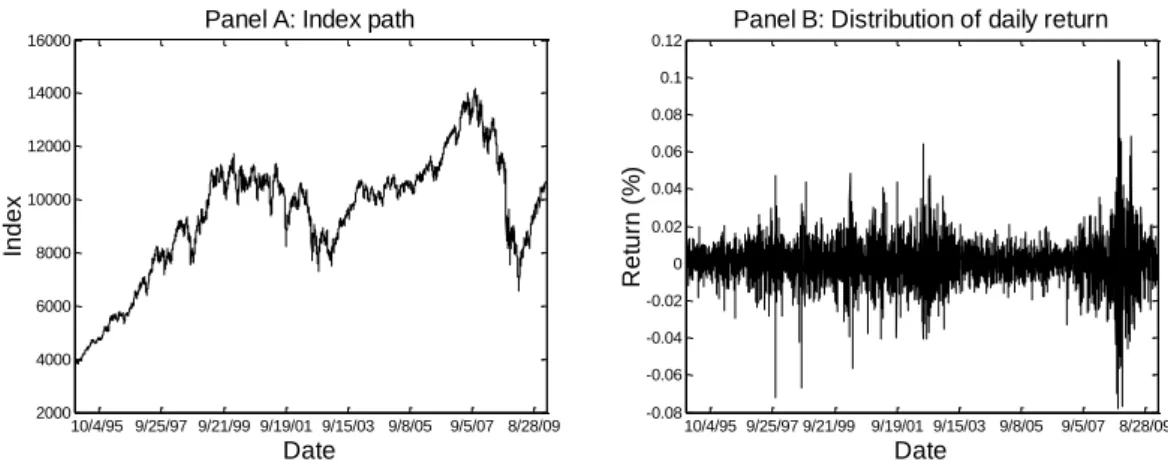
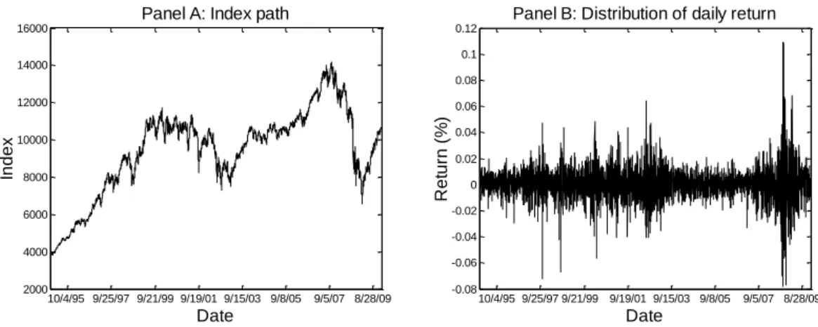
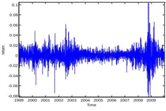
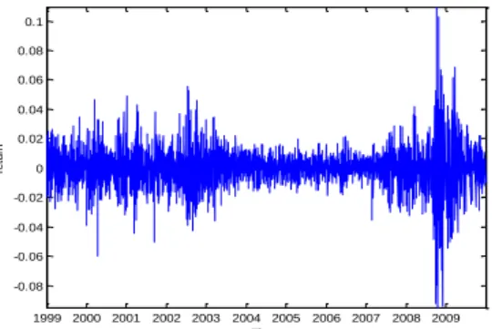
variables are continuous under a given regime. In brief, those studies ignore the discrete effects in describing the behavior of economic variables. To display the significance of such an effect, we take Dow Jones Industrial Average Index (hereafter DJIA) as an example. Figure 1 plots the index (Panel A) and daily returns (Panel B) of DJIA from Jan. 3rd, 1995 to Jan. 15th, 2010. The data of sudden shocks in DJIA daily return are given in Table 1.Weak, median, and strong shock are defined when the daily observation is over or below the level of single, double, and triple standard error of those computed by full period. From the Panel A of Figure 1, we observe that the index continues to grow during the period 1995-2000 due to the U.S. “new economy”, while in the second half of 2000,economyfaces the crash of Internet bubbles. The expansion from 2003 to mid-2007 is attributed to the effect of oil-shock-based inflation. Global subprime mortgage crisis, however, appears in 2008, and thus its aftermath prompts the nearest depression. Such an undulating pattern for the index path is the so-called “business cycle” which can be captured well by existing models.
Figure 1: DJIA index and its daily return from Jan. 3rd, 1995 to Jan. 15th, 2010
10/4/95 9/25/97 9/21/99 9/19/01 9/15/03 9/8/05 9/5/07 8/28/09 2000 4000 6000 8000 10000 12000 14000 16000
Panel A: Index path
Date In d e x 10/4/95 9/25/97 9/21/99 9/19/01 9/15/03 9/8/05 9/5/07 8/28/09 -0.08 -0.06 -0.04 -0.02 0 0.02 0.04 0.06 0.08 0.1 0.12
Panel B: Distribution of daily return
Date R e tu rn ( % )
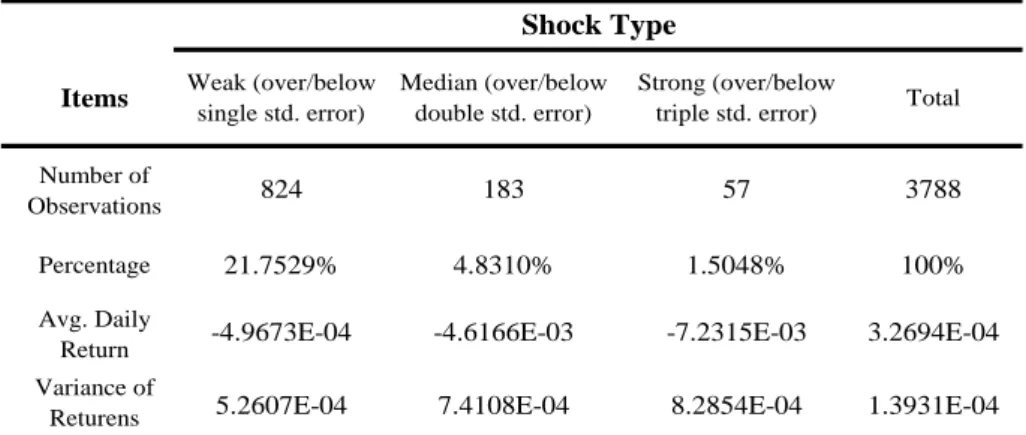
Table 1: Sudden shocks in the daily return of D.J.I.A. index from Jan. 3rd, 1995 to Jan. 15th, 2010
Compared to Panel B, it is notable that fluctuations in the daily return are fiercer visibly, especially at the time where abnormal events occur (e.g., subprime mortgage crisis). The numbers shown in Table 1 give a clearer insight to the sudden shocks. For example, the ratio of strong-shock observation to total is 1.5048%, which implies the likelihood of a strong sudden shock. Further, the means and variances of returns under shocks are also lower and higher respectively relative to those computed by full sample. These facts suggest that, as abnormal events strike the market, the index returns behave highly volatile within a short time period (e.g., 1 day). Such a nature of dynamic is obviously not in line with the usual assumptions that time-series variables act continuously. Hence, the family of existing Markov switching models cannot explicitly capture the impacts of sudden shocks. To explore this issue, our study tests whether the sudden shock is significant in market returns under switching regimes using NYSE data.
In 1976, Merton proposes the original type of jump-diffusion models.1 He assumes
1There has been a vast work on applying the jump-diffusion model in several dimensions; for example,
option pricing (Kou, 2002; Kou and Wang, 2004; Hilliard and Schwartz, 2005; Duan et al., 2006; Ahn et al., 2007; and Feng and Linetsky, 2008;), financing structure (Dao and Jeanblanc, 2006; and Chen and Kou, 2009;), time-series analysis (Becker, 1981; Ball and Torous, 1985; Akgiray and Booth, 1988; Jorion, 1988; Bates, 1996; Pan, 2002; Eraker, 2004; Jiang and Oomen, 2007, andLin,Wangand Tsai, 2009;), and term structure of interest rate and credit spreads (Ahn and Thompson, 1988; Duffie and Pan, 2001; Zhou, 2001; Das, 2002; Glasserman and Kou, 2003; Johannes, 2004; Guan et al., 2005;and
Items Weak (over/below
single std. error)
Median (over/below double std. error)
Strong (over/below
triple std. error) Total
Number of
Observations 824 183 57 3788
Percentage 21.7529% 4.8310% 1.5048% 100%
Avg. Daily
Return -4.9673E-04 -4.6166E-03 -7.2315E-03 3.2694E-04
Variance of
Returens 5.2607E-04 7.4108E-04 8.2854E-04 1.3931E-04
that total changes in the asset’s price can be divided between a normalvibration part and an abnormal vibration part. The former is modeled as a standard geometric Brownian motion with a fixed variance capturing continuous fluctuations in the prices because of strategic trading by informed or liquidity traders and the market microstructure effects; while the latter is modeled as a counting process that reflects discrete effects due to unanticipated information released to the public. To capture the sudden shock under switching regimes, this paper makes a combination of Markov regime-switching process with jump risks. Jumps in the model are assumed to obey a Poisson process with a constant jump rate. The methodology for estimation we adopt is Expectation-Maximization (hereafter EM) algorithm (see Dempster et al., 1977;), rather than traditional MLE. The main advantage of using EM algorithm over MLE is to overcome the problems of missing data and slow convergence (see Hamilton, 1990). Likelihood ratio test is also used in this study to compare the fitting performance of a standard-type regime-switching model with ours. The data we collect consist of 49 NYSE listed stocks, each with over 3500 daily observations spanning the period from Jan. 3rd, 1995 to Jan. 15th, 2010.
The structure of this study is organized as follows. In Section 2, models of stock return, including a regime-switching model with jump risks and a standard-type model, will be illustrated. Section 3 estimates the parameters via EM algorithm. Section 4 evaluates European options with a regime-switching model and a regime-switching model with jump risks. Numerical and empirical analyses are given in Sections 5. Section 6 draws the conclusion.
2. Model of Stock Returns
In the real world, the mean and volatility of a time series variable usually vary with market regimes. For instance, the mean of stock returns is positive in the bull
market but negative in the bear market, while its volatility is significantly higher during a pooreconomic condition. Such structural changes in the economic series cannot be captured by traditional models, which assume that all the observations on aparticular series are drawn from a Gaussian distribution with fixed mean andvariance throughout the sample period. Markov switching models are especially useful for addressing this issue.
2.1 Markov switching model
Consider a continuous trading economy. The uncertainty over this economy is defined on a finite space S consisting of states 1, 2, 3, , S. A standard-type Markov switching model governing the dynamic of stock returns with instantaneous mean
t
q
u and constant volatility
t
q
under the state qtS at time t1, 2,3,...,T
is one that attaches a hidden Markov process to Merton’s diffusion model:
t t
t q q t
R u Z (2.1)
where Rt denotes the stock return at time t; Zt plays a standard one-dimensional
normal distribution at t; and q implicates the unobservable state of economy at t t
characterized by a hidden Markov Chain on S.
Recall Markov properties which state that if the current state of the process is known, then the future behavior of the process is independent of its past (Klebaner, 1998;). Hence, the conditional probabilities of qt i and Rt must satisfy
1 1 1 ( t t , , ) ( t t ) P q i q q P q i q and 1 1 1 1 1 1 ( t t , t , , , ) ( t t , t ) P R R q R q P R R q .
Now we are ready to form the migration of q as a transition probability matrix t P
with pij P q( t1 j qt i) for i j, S and t 1, 2,3,...,T:
11 12 1 21 22 2 1 2 . s s s s ss p p p p p p P p p p
Note that the sum of each entry in the same row must equal one; namely,
1 1
s ij j p
for iS. To give the definition of initial state probability, let i p q( 1 i) that
satisfies 1 1 s i i
.When studying business cycle the uncertainty over economy is generally divided between expansion and recession. Hence, the standard Markov switching model can be reduced to a two-regime model (so-called “regime-switching model”). A growing economy is classified as in expansion (letting qt 1). In such a state 1
t q u u and 1 t q
. On the other hand, when the state is recession (i.e., qt 2), the value is taken as 2 t q u u and 2 t q
. Then we define a finite space containing all the
relevant parameters as { , , , 2 , , 2}
i p uij i i i j S s
.
It has been mentioned that Markov switching–type models are successful in explaining the asymmetric behavior of time series caused by changes in the structural state. This is becausethey produce leptokurtosis (fat fail) and skewness (nonzero third-order cross-moments) in the return (see Krolzig, 1997; and Solaand and Timmermann, 1998). Based upon our discussions, however, it is found that the arriving of unanticipated abnormal events delivers sudden shocks to the market, and hence the daily observations behave highly volatile within a short time period. Such
dynamic cannot be captured using existing models that usually assume that variables act continuously under a given regime. To address this issue, in the following subsection a regime-switching model with jump risks will be proposed.
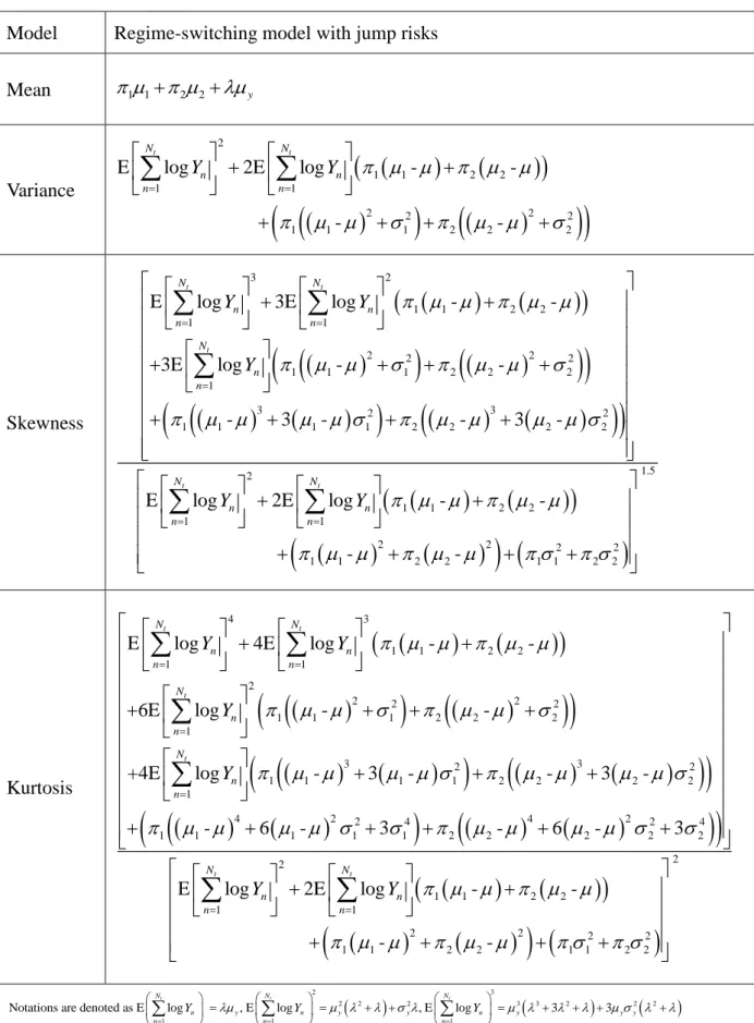
2.2 Regime-switching model with jump risks
The model we proposed makes the combination of a standard regime-switching process and a compound Poisson process N with constant intensity . First, let’s consider an infinite sequence ( )Yn n1,2,.., that consists of independent and identically distributed random variables representing the n -step jump size. A larger jump size
implies a fiercer shock; moreover, an upward jump indicates the release of unexpected good news. For tractability assume that all the jumps follow a lognormal distribution with constant mean and variance 2. Total number of jumps over the time period ( 0, ]t is counted using a Poisson process Nt. As usual, three sources of model’s
randomness ( )Yn n1,2,.., , (Nt t)0 , and (Zt t)0 are assumed to be mutually independent. The dynamic of returns on a stock governed by a switching regime with jump risks thus has the following explicit form
0log t t t N t q q t n n R u Z
Y (2.2) with a corresponding finite parameter space2 2
{ , , , , , , , , 2}
J i p uij i i i j S s
.
From Equ. (2.2) the volatility of stock return is decomposed into two parts: continuous vibrations and discrete vibrations. The former is modeled as a product of standard normal distributed variable and regime-switching variance; whilethe latter is described using a jump process reflecting non-marginal effect of the information.Our idea serves an extension of Merton’s jump-diffusion model. Differing from Merton,
however, the key role in the model is the regime-switching process, instead of a pure standard Brownian motion. The estimation of relevant parameters in two spaces and J will be discussed later.
3. Parameters Estimation via Expectation-Maximization Algorithm
This section gives the estimation of models’ relevant parameters. As for esti- mation, the generalized method of moments (GMM), originally proposed by Hansen (1982), is one of the most widely adopted techniques in jump-diffusion literature. The feature of GMM is based on moment conditions, which are still available even though the explicit form of probability density function sometimes is unknown. Due to this feature, it is convenient to use GMM for obtaining a single estimation quickly. As the total number of model parameters increases, however, GMM becomes ineffective since the heavy computation of higher-order moments is quite time-consuming. Further, several empirical researches (such as Kendall and Stuart, 1977; and Becker, 1981) indicate that GMM i likely to generate negative estimations for variances of stock returns. To overcome these issues, Ball and Torous (1985) implement MLE procedure in the parameter estimations.
MLE method has been very popular because of its great properties of consistency, invariance, and asymptotic normal distribution with large sample. Lobo (1999) is a typical case of using MLE with jump diffusion models to examine the political effects on stocks’ returns. Another well-established method is the Newton-Raphson procedure, which is especially useful for nonlinear estimations and multidimensional cases. These two methods, nevertheless, suffer from the restrictions of data missing and slow convergence. Hence, Hamilton (1990) numerically suggests the robust EM algorithm (originally proposed by Dempster et al., 1977). EM algorithm consists of
two stages: the first is “Expectation stage” (or E stage) that operates the conditional expectation of complete-data likelihood function given the observations and parameters of the last period; and the second called “Maximization stage” (or M stage) is to find the optimal estimations such that the conditional expectation of data likelihood function, yielded by first stage, reaches the maximum. Following Dempster et al., 1977 , and Lin et al, 2009, the method we adopted for estimation in this study is the EM algorithm.
3.1 Estimation under the standard regime-switching model
Given the model in Equ. (2.1), let R {R R1, 2,...,RT} be the set of observed
data and q {q q1, 2,...,qT} the set of missing data. Thus the set with complete data
follows that X { , }R q {R R1, 2,...,RT,q q1, 2,...,qT}. Also denoted by LC( R q, ), the explicit form of complete-data likelihood function is
1 -1 2 1 ( , ) ( , ) ( ) ( , ) t t T T C q q q t t t t L R q P R q P q p P R q
.This can be rewritten using log-operator as
1 1
2 2 2
,
2 1
log ( , ) log log 0.5 [ log ( 2 ( )) ( ) ]
t t t t t
T T
C q t q q t q t q q
L R q p R u
In the “E stage” of algorithm, we write down the expectation of data likelihood function conditioned on the observation to parameters at k 1 period (k 1):
2 ( 1) ( 1) ( 1) 1 1 2 2 ( 1) 1 1 1 2 2 ( 1) 1 1 ( ) log ( , ) ( , ) log ( , , ) log ( , ) T k k k t t t i t T k ij t t i j t k i i Q P R q i P q i R p P q i q j R P q i R (3.1) where the first line describes the dynamics of stock returns given different states of
the business cycle; the second line sketches the transition probabilities; and the third line expresses the conditional probabilities of initial states.
From the essence of EM algorithm, it is known that increasing Q( (k 1))
forces an increase in the log-likelihood of the observed data. Thus the second stage of algorithm is to produce a sequence of ( )k
that converges to maximum likelihood estimators. To this end, we proceed with the following steps. Firstly, using EM gradient algorithm in maximizing the dynamic in stock returns (first line in the right hand side of (3.1)), we have
( ) ( 1) 20 ( 1) 1 10 ( 1)
( ( ) ) ( )
k k k k
d Q d Q
where the parameter column vector at k period satisfies
( ) ( 1) arg max ( ) k k Q
andoperators d and 10 d20are the first- and the second-order partial derivation with respect to .Note that the Hessian matrix d Q20 ( (k 1)) must be negative and
definite such that the uniqueness of the maximum point ( )k and the strict concavity of Q( (k 1)) both can be ensured. For the detailed proof ofEM gradient algorithm, one can refer to Appendix A.
The maximization of transition probabilities (second line in (3.1)) is equivalent to solving a maximizing problem constrained by 2
1 ij 1 j p
. Using Lagrangian multiplier, we yield 2 ( 1) ( 1) 1 1 1 2 1 2 ˆij [ Tt ( t , t , k )][ j Tt ( t , t , k )] p
P q i q j R
P q i q j R .Similarly, to maximize initial probabilities (third line in (3.1)) subject to 2
1 i 1
i
,2 ( 1) ( 1) 1 1 1 1 ˆi ( , k )[ ( , k ) ] i P q i R P q i R
.The method we adopted for computing the above two terms
( 1) ( t , k ) P q i R and ( 1) 1 ( t , t , k ) P q i q j R is Baum-Welch algorithm (hereafter BM algorithm). To understand BM algorithm in the calculation, we define a forward probability and a backward probability first, and then introduce the forward and the backward algorithm. Let ( )ik( )t denotes the forward probability of stock
return series R1 r1,...,Rtrt at time t under the stateqt i; namely,
( ) ( 1) 1 1 ( ) ( ,..., , ) k k i t P R r Rt r qt t i ,
while i( )k ( )t denotes the corresponding backward probability
( ) ( 1) 1 1 ( ) ( ,..., , ) k k i t P Rt rt RT rT qt i .
Also let b( )ik (R denote the density function for the probability that time-t) tstock return is at level rt given the state qt i:
( ) ( 1) ( 1) 2 0.5 ( 1) 2 ( 1) 2 ( ) ( , ) [ 2 ( ) ] exp ( 0.5( ) ( ) ) k k i t t t t k k k i t i i b R P R r q i r u
The standard procedure of the forward process algorithm is shown as below: initial, ( ) ( ) ( ) 1 (1) ( ) k k k i i bi R . (3.2) recursive, 2 ( ) ( ) ( ) ( ) 1 1 ( 1) ( ) ( ) k k k k j t bj Rt i i t pi j
. (3.3) termination, ( 1) 2 ( ) 1 ( ) ( ) k k i i P R T
. (3.4) The similar procedure for the backward process algorithm is( ) ( ) 1 k i T . (3.5) recursive, 2 ( ) ( ) ( ) ( ) 1 1 ( ) ( ) ( ) ( 1) k k k k i t j pi j t bj Rt j t
. (3.6) termination, ( 1) 2 ( ) ( ) ( ) 1 1 ( ) (1) ( ) k k k k i i i i P R b R
. (3.7) However, it is notable that such a standard procedure may suffer from the underflow problem.To overcome this restriction, this study applies the method proposed by Durbin et al. (1998) to adjust the form of forward and backward probabilities. That is,( ) ( ) 1 1 1 1 ( ) ( ) ( T ) k k i t i t t ct
and ( ) ( ) 1 1 1 1 ( ) ( ) ( T ) k k i t i t t t
gwhere (ct1)Tt1 1 and(gt1)Tt1 1 both denotes a sequence ofpositive number satisfying
2 ( ) 1 ( ) 1 , 1,..., k i i t t T
and 2 ( ) 1 ( ) 1 , 1,..., k i i t t T
.Thus, putting (3.2)-(3.7) into i( )k ( )t and i( )k ( )t yield the adjusted algorithm procedure: (i) the forward process algorithm, for 2 2 ( ) ( ) ( )
1 1 1 ( 1) ( ) k k k t j i j t i i j c
b R t p and 2 ( ) ( ) 1 1 ( 1) k k i i i c
b R , initial, ( ) ( ) ( ) 1 1 1 (1) ( ) ( ) k k k i bi R i c recursive,2 ( ) ( ) 1 ( ) ( ) 1 1 1 ( 1) ( ) ( ) ( ) k k k k j t bj Rt ct i i t pi j
termination, ( 1) 1 ( k ) T t t P R
cand (ii) the backward process algorithm, for 2 2 ( ) ( ) ( )
1 1 ( ) ( 1) .
k k k
t j i j t i i j
c
b R t p3.2 Estimation under the regime-switching model with jump risks
We now repeatthe use of EM algorithm for the parameter estimation in the presence of jump risks. Firstly R {R R1, 2,...,RT}denotes the set ofobserved data,
and q {q q1, 2,...,qT}and N={N1,N2,...,NT} both the missing data. Under a regime-switching model with jump risks, the complete-data likelihood functionis thus
1 -1 2 1 1 ( , , ) ( , , ) ( ) t t T T T J C J q q q t t t J t J t t t L R q N p P R q N P N
or, in the log-form
1 1 , 1 1
2 2 2 2 2 1
1
log ( , , ) log log [ log log ( !) ]
0.5 [ log ( 2 ( ) ) ( ) ( ) ] t t t t t T T J C J q t q q t t t T q t t q q t t L R q N p n n n R u n
Conditioned on the observation of relevant parameters atk 1 period J(k 1), taking expectation operator gives
( 1) ( 1) 2 ( 1) ( 1) 1 1 0 2 2 ( 1) 1 1 1 1 ( 1) 1 0 ( ) ( log ( , , ) , ) log ( , ) ( , ) ( , ) log ( , , ) log ( , ) ( , ) t t k J k J J C J J T k k t t t J t J i t n T k ij t t J i j t T k t t t t t t J t n Q E L R q N R h n P N n R P q i R p P q i q j R P R q i N n P N n R 2 1 ( 1) 2 ( 1) 1 1 ( , ) log ( , ) i k t J k i J i P q i R P q i R (3.2)
Note that differences between (3.1) and (3.2) mainly lie in two terms: h n( t, ) and
( 1)
( t t , Jk )
P N n R , where the former is a Poisson density function with constant intensity , while the latter denotes the conditional probability of a Poisson process
2 ( 1) ( 1) ( 1) 1 ( 1) 2 ( 1) ( 1) ( 1) 1 0 ( , , ) ( ) ( ) ( , ) ( , , ) ( ) ( ). t t t k k k t t t t J t t J t J q k t t J k k k t t t t J t t J t J q n P R N n q P N n P q P N n R P R N n q P N n P q
Then, in M stage, with a similar procedure in (3.2) (including Lagrangian multiplier and EM gradient algorithm), we havethe same procedure with M stepin 3.2 subsection.
4. Option Pricing under Business Cycle with Jump Risks
This section firstly introduces the option pricing under business cycles, then further consider option pricing underbusiness cycles with jump risks.
4.1 Option pricing under the regime-switching model
Consider the following dynamic process of the stock price under regime-switching model
t t q q dS dt dW t S where qt 1, 2denotes the states of the business cycles. Therefore, let the stockpricebeS(0) attime 0, then the stockprice at timet can be written as
2
0 0 0 1 0 exp -2 t t t T T T q q q S T S dt dt dW t
1 2
1 2 1 1 1 1 2 1 0 t 0 1 1 T ( ) T T qdt D qdt q dt T q dt D D T D
1 2
1 2 2 2 2 2 2 2 1 1 1 1 2 1 0 t 0 1 1 T ( ) T T qdt D qdt q dt T q dt D D T D
1 2 1 2 1 1 0 0 1 1 1 1 2 1 t T T T qdW t D qdW t q dW t T q dW t D W D W T D
Under business cycle, we collect the state 1 all of the W t
W t
1
become
1W D .Similarly, we collect the state 2 all of the W t
W t
1
become
1
W TD .Therefore, when state 1 isD ,the dynamics of the stock price at time Tis 1
2 2
1 1 2 1 1 1 2 1 1 1 2 1 1 0 exp ( ) - ( ) 2 S T S D T D D T D W D W TD According the payoff of European option, the value of the option is the discounted payoff (by the risk-neutral measure) shown as follows,
1 1 1 1 -> -1 ln > ln 0 0 -1, 2, max - , 0 - I 0 - I 0 0 S 0 rT Q rT Q S T K rT D Q S T K S S rT D D D RSC E e S T K E e S T K S T K E E e S D S S E d Ke d where ( ) denotes the cumulative distribution function of the standard normal distribution, and
1 2 2 1 1 2 1 1, 2 2 1 1 2 1 0 1 ln ( ) 2 , ( ) D S rT D T D K d D T D
1 2 2 1 1 2 1 2, 2 2 1 1 2 1 0 1 ln ( ) 2 ( ) D S rT D T D K d D T D .Consider that the stock price depends on the business cycles and relevant information as follows
1 -1 t t N t q q n n dS dt dw t d Y S
,where qt 1, 2 denotes the state of business cycle,
N t
presents the number of the jump event at interval [0, t] and is the arrival rate of the information.
Y ndenotes the jump size for the stock price when the information arrives, and we assume that the jump size follows lognormal distribution with location parameter, y, and
scale parameter, 2 y
, respectively. Then, at time T, the stock price is
2 0 0 0 1 2 0 0 0 1 1 0 exp -2 1 0 exp - log 2 t t t t t t N T T T T q q q n n N T T T T q q q n n S T S dt dt dW t Y S dt dt dW t Y
Therefore, when D isstate 1, the dynamics of the stock price at time Tis 1
2 2 2 1 1 2 1 1 1 2 1 1 1 2 1 1/ 2 1 1 0 exp ( ) - ( ) 2 + log ( y y 1) N T u n n S T S D T D D T D W D W T D Y T e
where W D sum of the
1 W t
W t
1
atstate 1; W T
D1
sum of the
1
W t W t at state 2.
According the payoff of European option, the value of the option is the discountedpayoff(by the risk-neutral measure) shown as follows
- -> max - , 0 - I rT rT Q Q S T K RSPJCE e S T K E e S T K
1 2 1 1 1 2 1 1 -, ( ) 1 ln > ln 0 0 2 -, ( ) 1, , 2, , 2 -1, , 0 0 - I , ( ) 0 0 0 0 ! y y y y rT D N T Q S T K S S m rT D N T D m D m m T m rT D D m m S T K E E e S D N T m S S E S e d Ke d e T E S e d Ke m
1 2,D m, d where ( )denotes the cumulative distribution function of the standard normal distribution, 1 1,D m, d and 1 2,D m,
d are presented as follows
1 2 2 2 1 1 2 1 1, , 2 2 2 1 1 2 1 0 1 ln ( ) 2 y y D m y S rT D T D m K d D T D m ,
1 2 2 1 1 2 1 2, , 2 2 2 1 1 2 1 0 1 ln ( ) 2 y D m y S rT D T D m K d D T D m .5. Empirical and Sensitivity analysis
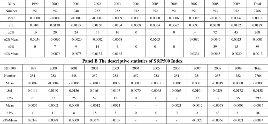
Our daily return sample is drawn from the Dow Jones index 30 component stocks, including during the period from 1999 to 2008.Therefore, there are 2515 observations for each stock. We adopt a log return approach to calculate the daily stock return as follows
1 ln t t t S R S
whereStis stock price at timet.
In this section, we first present the descriptive statistics of Dow Jones Industrial Average Index and component stock returns.We then estimate the parameters in the
Black-Scholes model under the condition of Markov switching model and Markov switching model with jump risks.Finally, we test (1) if stocks returns follow Markov switching model, which shows the impact of business cycles; (2) if stocks returns follow Markov switching model with jump risk, which presents the impact of business cycles with jump risk. Finally, we analyze the impact of model parametersincorporating business cycles with jump risks on the pricing of options.
5.1 Descriptive statistics
First, we analyze DJ-30 component stocks using descriptive statistics. In Table 1, we assume the economy is in a booming state if mean returnis larger than -0.0001 and variance is smaller than 0.0120; otherwise it is a contraction state.Given this definition,then 1999 and 2003-2007 is clearly booming years, and 2000-2002 and 2008 contracting years which correspond to the internet bubble and subprime crisis periods – consistent with the official definition of business cycles.Furthermore, we observe a jump whenever the stock return is greater than ±2%. Obviously, jumps are observed irrespective of business cycles. Hence, from table 1, our proposal of a model with business cyclesincorporating jump risks is reasonable.
5.2 Empirical analysis
Since Black-Scholes model assumes stocks returns follow log-normal distribution, hence average return and sample standard deviation are used to estimate population parameters. However, Markov switching model considers different economic conditions, hence the stock returns follow normal distributions of various parameters, i.e., p ,11 p ,22 1,2 ,1and2. Where p stands for the 11
probability of Markovchain to remain in state 1; p stands for the probability of 22
Markovchain to remain in state 2;1 and2stand for the growth rate of stock returns at state 1 and 2, respectively;while 1 and2stand for the volatility of stock returns
at state 1 and 2, respectively. In addition, the Markov switching model with jump risks not only considers business cycles but also considers stock price jump.The estimate parameters are thus p ,11 p ,22 1,2,y,1,2,y and
, where ystands for average jump size under the prerequisite of the jump volatility.; ystands for thestandard deviation of jump size;
stands for jump frequency; other parameters are the same as previously stated in the Markov switching model. Because business cycles and jump frequency are hidden Markova chain, this paper adopt EM algorithm to estimate the MLE of state switching model parameters, which are consistent estimators and near normally distributed.From Section 5.1 we anticipateDJ-30 component stocks follow Markov switching model or Markov switching model with jump risks. Therefore, we propose the following hypotheses to test if indeed stock returns better fit these models.
Hypothesis 1
H0:Stock returns follow Black-Scholes model H1:Stock returns follow Markov switching model. Hypothesis 2
H0:Stock returns follow Markov switching model
H1:Stock returns follow Markov switching model with jump risks.
This paper uses MLE to test the above two hypothesis. The test statistics of hypothesis 1 follow a Chi-square distribution with degree of freedom 4, stated as follow ) 4 ( ~ ) ˆ , ( ) ˆ , ( ln 2 2 1 RS BS R L R L
) 3 ( ~ ) ˆ , ( ) ˆ , ( ln 2 2 2 RSJ RS R L R L
whereˆBSis the set of MLE for the Black-Scholes model;ˆRSisthe set of MLEfor the Markov switching model; ˆRSJis the set of MLE for the Markov switching model with jump risks;1 and 2 represent the test statistics for Hypothesis 1 and 2with a Chi-square distribution (degrees of freedom 4 and 3), respectively.
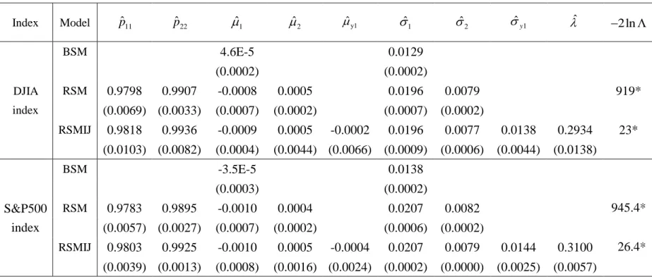
Table 3 exhibits the test results for 30DJ component stocks. Using EM algorithm to estimate the parameters of Markov switching model, we reject the null hypothesis of Hypothesis at less than 1% significance level, suggesting that Dow Jones component stock returns better fit the Markov switching model. Using Alcoa as an example, the results of parameter estimates show that switching probabilities are
11 0.7925
p andp220.9896, respectively, implying that Alcoa stock returns are affected by business cycles. The probability of switching from state 1 to state 2 is higher than switching from state 2 to state 1 implying longer duration of booming economy in long term. Alcoa’s average daily stock returns is -1.30% with a volatility of 11.92% in economic recession and the same statistics are -0.01% and 2.18%;in booming economy. Furthermore, results in Table 3 also reject the null of Hypothesis 2 at less than 1% significance level. This result shows that DJ component stocks follow Markov switching model with jump risks. Using Alcoa as an example again, the estimated parameters show that average jump size isy 0.0001, the standard
deviation of jump size isy 0.0173, and jump frequency is
1.5313.These statistics imply that the average daily jump is 1.5313 times with a jump size of 0.0001 each jump. This illustrates the existence of jump volatility in daily stock returns. Based upon the empirical results, we argue that the DJ-index and its componentstocks returns exhibit characteristics of business cycles and jump volatility. Under this event, Black-Scholes model will result in biased estimation of option values. In the next section, we will offer the parameters of pricing formula, the calculation of the theoretical value of a European call, and discussions of the impact of parameters on call values.
5.3 Sensitivity analysis
Because the DJ component stocks exhibit state switching phenomenon, this section performs sensitivity analysis assuming that two states Brownian motion volatility of Markov switching model are 14%, 2 1%, and the switch
probabilities are p110.90and p22 0.95, respectively. Tables 3 and 4report sensitivity analysis of European call price assuming stock returns follow Markov switching model. The base volatilityof state 1 ±2% and the basic volatilityof state 2 2% show the effect of the volatility of the Brownian motion. Hence, the volatility of daily stock return are 2%, 4% and 6% for state 1;and 0.5%, 1% and 2% for state 2. According to the sensitivity analysis of Table 3, other things held constant, there is a positive relationship between volatility and option value in state 1 and state 2, implying the larger the volatility, the higher the probability of increasing stock price, hence higher call price. In addition, other things held constant, there is a positive relationship between p and call value. The higher the11 p , the lower the probability 11
that the economy will switch from state 1 to state 2.That is, in the long term, the longer the duration of state 1, which has higher volatility, the higher the call value will be.On the contrary, there is a negative relationship between p and call value.The 22
1.In the long term, the longer the duration of state 2,which has lower volatility, the smaller the call value.
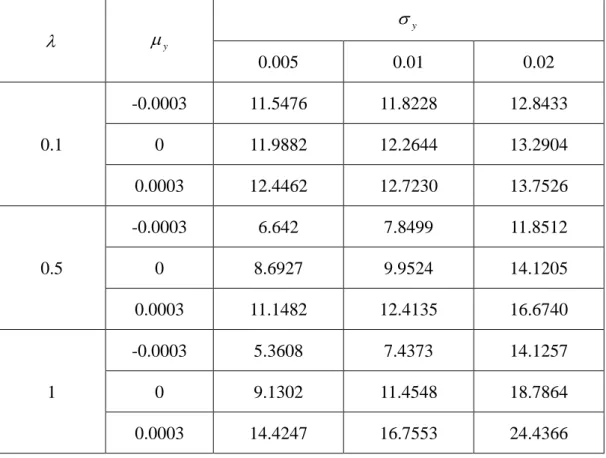
This paper also discusses the influence of jump volatility on call price. Table 5 illustrates the sensitivity analysis of the impact of jump size and jump frequencyon call price.Other things held constant, there is a positive relationship between average jump size and call price. Since call price increases at expiration when stock price increases, the bigger jump size implieslarger stock price upside volatility, hence higher call price.
The relationship between the standard deviation of jump size and call price is positive. The larger the standard deviation of jump size suggests higher probability of stock upside volatility, hence higher call price. Finally, other things held constant, there is no significant relationship between jump frequencyand call price. Although the higher jump frequency indicatesmore frequent jump volatility, theimpact on stock pricesdepends on jump size per jump; hence no relationship between jump frequency and call price.
6. Conclusion.
This paper develops option pricing model of business cycles with jump risks. Our results indicate that it is reasonable to incorporate business cycles with jump risk in the model. The empirical results show that all of the 30 DJ component stocks exhibit characteristics of jump risks and business cycle. Numerical analysis demonstrates the impact of business cycles and jump risks on option pricing.
Reference
returns.”The Journal of Financial and Quantitative Analysis. 18, 53-65.
Becker, S. 1981. “A note on estimating the parameters of the diffusion jump model of stock returns.”Journal of Financial and Quantitative Analysis. 16, 127-139. Chen, S. S.2007.“Does monetary policy have asymmetric effects on stock
returns?”Journal of Money, Credit and Banking, 39(2-3), 667-688.
Dempster, A.P., Laird, N.M., and Rubin, D.B. 1977. “Maximum likelihood from incomplete data via the EM algorithm.”Applied statistics. 39, 1-38.
Durbin, R., Eddy, S., Krogh, A. and Mitchison, G. 1998. “Biological sequenceanalysis: probabilistic models of proteins and nucleic acids.”CambridgeUniversity Press. Hamilton, J.D., 1989. “A new approach to the economic analysis of nonstationary
time series and the business cycle.” Econometrica,57, 357-384.
Hamilton, J. D. 1990. “Analysis of time series subject to changes in regime.”Journal
ofEconometrics. 45, 39-70.
Hamilton, J. D. and Susmel, R. 1994. “Autoregressive conditional heteroskedasticity and changes in regime.” Journal of Econometrics, 64, 307-333.
Kendall, M., and Stuart, A. 1977. “The advanced theory of statistics.”New York: MacMillan Publishing Company.
Kim, C.J., 1994. “Dynamic linear models with Markov-switching.”Journal of
Econometrics 60, 1-22.
Kim, C. J., Morley, J. C., and Neleson, C. R. 2005. “The structural break in the equity premium.” Journal of Business & Economic Statistics, 23, 181-191. Krolzig, H. M. 1997. “Markov-switching vector autoregressions:modeling, statistical
inference, and application to business cycleanalysis.”Berling: Springer-Verlag Press.
Lin, S. K., Wang, S. Y., Tsai, P. L.,(2009), “Application of hidden Markov switching moving average model in the stock markets: Theory and Empirical Evidence,”
International Review of Economics and Finance, 18(2),306-317.
Lobo, B., J. 1999. “Jump risk in the U.S. stock market: evidence using politicalinformation.”Review of Financial Economics. 8, 149-163.
Maheu, J. M., and McCurdy, T. H. 2000. “Identifying bull and bear markets instock returns,” Journal of Business & Economic Statistics, 18(1), 100–112.
Sola, M., and Timmermann, A. 1998. “Fitting the moments: acomparison ofARCH and regime switching models for daily stock return.”UCSD Working Paper. Wang, S. Y.,Lin, S. K., (2010),“The Pricing and Hedging of Structured Notes with
Systematic Jump Risk: An Analysis of the USD Knock-Out Reversed Swap,”International Review of Economics and Finance, 19, 106-118.
Turner, C. M., R., Startz, and Nelson. C. R. 1989. “A Markov model of heteroscedasticity, risk and learning in the stock market.”Journal of Financial
Table1 The descriptive statistics of the Dow Jones Industrial Average Index
Dow Jones 1999 2000 2001 2002 2003 2004 2005 2006 2007 2008 Total
Number 251 252 248 252 252 252 252 251 251 253 2514
Max 0.0280 0.048096 0.043719 0.061547 0.035276 0.017379 0.020389 0.019603 0.025223 0.105083 0.1051 Min -0.0263 -0.05822 -0.07396 -0.04751 -0.03672 -0.0165 -0.01878 -0.0198 -0.03349 -0.08201 -0.0820 Mean 0.0009 -0.00025 -0.0003 -0.00073 0.000896 0.000123 -2.4E-05 0.000601 0.000248 -0.00163 -1.81E-05 Variance 0.0102 0.013089 0.013505 0.016035 0.010431 0.00683 0.006488 0.006215 0.009179 0.023816 0.0126 Skewness 2.8665 4.680199 6.959033 4.186146 4.087145 2.864236 3.022708 4.19033 4.579914 6.726851 -0.0073 Kurtosis 0.0431 -0.2812 -0.56799 0.49053 0.111687 0.00947 -0.0031 -0.10916 -0.61948 0.22201 11.3385 up >2% 10 13 12 24 10 0 1 0 5 32 107 down>2% 6 18 12 24 5 0 0 0 9 40 114 up and down>2% 16 31 24 48 15 0 1 0 14 72 221
Table2The empirical analysis of the estimating and testing in the Black-Scholes model, the regime-switching model, the regime-switching model with Poisson jump risks
Name Model ˆp 11 ˆp 22 ˆ1 ˆ2 ˆy ˆ1 ˆ2 ˆy ˆ
Alcoa
BSM -0.0007 0.0338
(0.0007) (0.0005)
RSM 0.7925 0.9896 -0.0130 -0.0001 0.1192 0.0218 2790**
(2.37E-03) (7.23E-06) (1.24E-04) (2.07E-07) (2.51E-02) (1.20E-03)
RSMJ 0.9278 0.9982 -0.0391 -0.0002 1.32E-04 0.1519 0.0098 0.0173 1.5313 213** (4.03E-02) (1.05E-03) (1.83E-02) (6.58E-04) (6.49E-04) (1.53E-02) (7.94E-04) (1.88E-04) (6.76E-03)
American Express
BSM -0.0007 0.0325
(0.0006) (0.0005)
RSM 0.8882 0.9893 -0.0112 0.0003 0.0916 0.0186 2801**
(7.72E-04) (7.74E-06) (4.02E-05) (1.59E-07) (1.56E-02) (1.51E-03)
RSMJ 0.9308 0.9960 -0.0159 -0.0001 1.48E-04 0.1047 0.0064 0.0163 1.3839 165** (2.46E-02) (1.59E-03) (9.09E-03) (2.40E-04) (3.63E-04) (3.73E-04) (3.91E-04) (3.74E-04) (2.31E-02)
Name Model ˆp 11 ˆp 22 ˆ1 ˆ2 ˆy ˆ1 ˆ2 ˆy ˆ
AIG
BSM -0.0017 0.0401
(0.0008) (0.0006)
RSM 0.8540 0.9835 -0.0142 -0.0002 0.1157 0.0158 3914**
(8.48E-04) (1.14E-05) (5.28E-05) (1.17E-07) (1.13E-02) (1.55E-03)
RSMJ 0.9569 0.9978 -0.0260 -0.0004 -5.34E-06 0.1581 0.0082 0.0193 0.7762 156** (2.11E-02) (1.03E-03) (1.23E-02) (7.05E-04) (2.97E-03) (1.12E-02) (2.69E-04) (1.31E-04) (2.98E-02)
Boeing
BSM 0.0001 0.0213
(0.0004) (0.0003)
RSM 0.9740 0.9849 -0.0010 0.0008 0.0301 0.0136 808**
(3.91E-05) (1.49E-05) (9.86E-07) (1.35E-07) (3.88E-03) (2.93E-03)
RSMJ 0.9844 0.9919 -0.0010 0.0007 -9.56E-06 0.0279 0.0104 0.0107 0.8897 241** (6.11E-03) (6.67E-03) (1.02E-04) (1.38E-03) (3.73E-03) (3.29E-03) (1.39E-03) (1.84E-03) (3.06E-02)
Caterpillar
BSM -2.34E-05 0.0256
(0.0005) (0.0004)
RSM 0.7765 0.9859 -0.0050 0.0003 0.0771 0.0180 1659**
(2.14E-03) (1.26E-05) (4.30E-05) (1.46E-07) (2.35E-02) (1.44E-03)
RSMJ 0.8600 0.9949 -0.0139 0.0003 4.89E-05 0.0897 0.0110 0.0149 1.1046 117** (4.04E-02) (8.40E-04) (9.86E-03) (4.01E-03) (3.89E-03) (9.74E-03) (6.15E-04) (3.80E-04) (6.37E-02)
Name Model ˆp 11 ˆp 22 ˆ1 ˆ2 ˆy ˆ1 ˆ2 ˆy ˆ
Citigroup
BSM -0.0008 0.0311
(0.0006) (0.0004)
RSM 0.9348 0.9759 -0.0026 -0.0001 0.0555 0.0134 2785**
(2.35E-04) (2.57E-05) (4.31E-06) (1.03E-07) (5.96E-03) (3.61E-03)
RSMJ 0.9516 0.9916 -0.0049 -0.0002 8.23E-05 0.0639 0.0056 0.0122 1.5821 25** (1.41E-02) (2.60E-03) (3.11E-02) (3.85E-03) (2.91E-03) (1.36E-02) (1.20E-04) (7.84E-04) (1.43E-02)
Coca Cola
BSM -0.0002 0.0162
(0.0003) (0.0002)
RSM 0.9766 0.9823 -0.0008 0.0004 0.0227 0.0081 954**
(6.37E-03) (4.39E-03) (6.75E-04) (2.33E-04) (6.31E-04) (2.20E-04)
RSMJ 0.9819 0.9881 -0.0010 0.0002 0.0001 0.0219 0.0041 0.0053 2.0312 38** (5.32E-03) (3.72E-03) (7.92E-04) (7.59E-04) (1.95E-03) (5.14E-03) (4.46E-05) (3.34E-04) (7.64E-03)
Disney
BSM -0.0001 0.0226
(0.0005) (0.0003)
RSM 0.9660 0.9816 0.0001 -0.0002 0.0337 0.0130 1204**
(7.96E-05) (2.02E-05) (1.31E-06) (1.15E-07) (3.98E-03) (2.81E-03)
RSMJ 0.9788 0.9898 -0.0001 -0.0003 2.85E-05 0.0322 0.0075 0.0085 1.9004 141** (1.41E-02) (9.57E-04) (1.06E-03) (4.87E-04) (1.51E-07) (9.33E-04) (6.57E-04) (5.38E-04) (2.78E-03)
Name Model ˆp 11 ˆp 22 ˆ1 ˆ2 ˆy ˆ1 ˆ2 ˆy ˆ
Du Pont
BSM -0.0003 0.0194
(0.0004) (0.0003)
RSM 0.9750 0.9857 -0.0008 -4.22E-05 0.0279 0.0119 344**
(1.41E-04) (2.65E-05) (8.54E-07) (1.05E-07) (8.40E-03) (4.15E-03)
RSMJ 0.9708 0.9882 -0.0005 -0.0002 -2.26E-05 0.0286 0.0077 0.0078 1.6726 243** (1.07E-03) (3.31E-03) (8.33E-02) (7.12E-03) (1.01E-02) (8.35E-03) (6.83E-04) (3.82E-04) (1.28E-02)
Exxon Mobil
BSM 3.77E-05 0.0223
(0.0004) (0.0003)
RSM 0.8461 0.9952 -0.0075 0.0003 0.0970 0.0148 970**
(2.82E-03) (3.16E-06) (1.28E-04) (9.20E-08) (3.81E-02) (1.03E-03)
RSMJ 0.9063 0.9918 0.0004 0.0005 3.17E-05 0.0466 0.0118 0.0052 1.9006 175** (2.72E-02) (5.73E-04) (4.87E-02) (3.70E-03) (1.95E-03) (1.10E-02) (3.40E-04) (2.91E-03) (1.61E-02)
General Electric
BSM -0.0007 0.0300
(0.0006) (0.0004)
RSM 0.8655 0.9906 -0.0100 -0.0001 0.1013 0.0154 2471**
(1.15E-03) (6.24E-06) (6.41E-05) (1.05E-07) (1.74E-02) (1.26E-03)
RSMJ 0.9064 0.9948 -0.0116 -0.0004 1.50E-04 0.0996 0.0058 0.0120 1.5656 122** (2.86E-02) (1.47E-03) (4.55E-01) (2.11E-04) (6.29E-05) (5.93E-03) (1.07E-04) (2.32E-04) (2.50E-02)
Name Model ˆp 11 ˆp 22 ˆ1 ˆ2 ˆy ˆ1 ˆ2 ˆy ˆ General Motors BSM -0.0012 0.0325 (0.0006) (0.0005) RSM 0.8703 0.9811 -0.0046 -0.0007 0.0741 0.0202 2681**
(5.97E-04) (1.50E-05) (1.80E-05) (1.90E-07) (1.18E-02) (1.95E-03)
RSMJ 0.9404 0.9947 -0.0105 -0.0009 8.97E-05 0.0810 0.0078 0.0147 1.9796 135** (5.20E-03) (1.73E-03) (1.64E-01) (2.47E-02) (8.08E-03) (5.44E-02) (5.03E-04) (1.42E-03) (5.00E-02)
Hewlett Packard Company BSM -0.0003 0.0306 (0.0006) (0.0004) RSM 0.9591 0.9761 -0.0013 0.0003 0.0461 0.0154 2677**
(8.77E-05) (2.73E-05) (2.32E-06) (1.69E-07) (3.14E-03) (2.57E-03)
RSMJ 0.9891 0.9903 -0.0009 0.0006 -6.44E-03 0.0328 0.0141 0.1019 0.0236 293** (7.09E-03) (4.52E-03) (2.40E-03) (1.59E-03) (1.13E-02) (1.67E-03) (8.42E-04) (4.10E-02) (1.12E-03)
Home Depot
BSM -0.0004 0.0253
(0.0005) (0.0004)
RSM 0.9743 0.9864 -0.0016 0.0003 0.0382 0.0143 1764**
(5.90E-05) (1.60E-05) (1.72E-06) (1.36E-07) (3.74E-03) (2.63E-03)
RSMJ 0.9801 0.9898 -0.0013 1.78E-05 -1.82E-05 0.0349 0.0074 0.0092 1.9054 132** (9.47E-03) (6.58E-03) (2.83E-02) (3.87E-03) (4.84E-03) (9.43E-03) (4.01E-04) (3.58E-03) (1.72E-01)
Name Model ˆp 11 ˆp 22 ˆ1 ˆ2 ˆy ˆ1 ˆ2 ˆy ˆ Honeywell Internation al BSM -0.0001 0.0239 (0.0005) (0.0003) RSM 0.9565 0.9833 -0.0015 0.0004 0.0388 0.0146 1460**
(8.90E-05) (1.23E-05) (2.28E-06) (1.29E-07) (4.61E-03) (2.23E-03)
RSMJ 0.9718 0.9904 -0.0023 0.0003 5.32E-05 0.0362 0.0067 0.0095 2.1357 122** (4.12E-03) (1.20E-03) (2.91E-02) (1.67E-02) (8.56E-03) (5.11E-03) (4.50E-04) (1.37E-04) (4.32E-02)
Intel
BSM -0.0008 0.0357
(0.0007) (0.0005)
RSM 0.9270 0.9859 -0.0078 0.0006 0.0730 0.0214 3065**
(1.59E-04) (1.15E-05) (1.32E-05) (2.43E-07) (5.06E-03) (1.44E-03)
RSMJ 0.9982 0.9983 -0.0003 0.0005 -1.46E-01 0.0360 0.0164 0.2314 0.0066 554** (1.29E-03) (1.25E-03) (4.00E-03) (8.58E-04) (2.12E-02) (8.21E-04) (4.19E-04) (3.24E-03) (1.97E-03)
IBM
BSM -0.0003 0.0247
(0.0005) (0.0003)
RSM 0.9576 0.9821 -0.0020 0.0004 0.0412 0.0116 1666**
(1.23E-04) (1.89E-05) (2.26E-06) (8.62E-08) (4.30E-03) (2.22E-03)
RSMJ 0.9891 0.9930 -0.0011 0.0006 -2.28E-04 0.0277 0.0079 0.0130 0.4492 218** (2.86E-03) (1.53E-03) (9.68E-03) (9.41E-03) (3.48E-03) (2.71E-03) (5.30E-05) (3.46E-03) (2.22E-03)