Synthesis of a robust broadband duct ANC system using convex
programming approach
Mingsian R. Bai and Pingshun Zeung
Department of Mechanical Engineering, National Chiao-Tung University, 1001 Ta-Hsueh Road, Hsin-Chu 30010, Taiwan, Republic of China
共Received 24 July 2000; revised 27 August 2001; accepted 17 January 2002兲
A robust active controller using spatially feedforward structure is proposed for broadband attenuation of noise in ducts. To meet the requirements of performance and robust stability in the presence of plant uncertainties, an H2 cost function and an H⬁ constrain are employed in the synthesis of the controller. The design is then converted into a convex programming problem using Q-parametrization and frequency discretization. An optimal controller that satisfies the quadratic cost functions and linear inequality constraints can be found by sequential quadratic programming. The optimal controller was implemented via a digital signal processor 共DSP兲 and verified by experiments. Experiment results showed that the system attained 16.5 dB maximal attenuation and 5.9 dB total attenuation in the frequency band 200– 600 Hz. © 2002 Acoustical Society of America. 关DOI: 10.1121/1.1460926兴
PACS numbers: 43.50.Ki关MRS兴
I. INTRODUCTION
Active noise control 共ANC兲 offers numerous advan-tages, e.g., compact size and low-frequency performance, over conventional passive technologies. Although the adap-tive feedforward control, e.g., the filtered-X algorithm is widely used, fixed controllers based on optimal control and robust control are gaining research attention in the field of ANC. Many design techniques have been applied to the duct ANC problem for synthesizing fixed controllers. Hong et al.1 and Wu et al.2investigated the duct ANC problem using the linear quadratic Gaussian 共LQG兲 control. Along the same line, robust controllers are designed using combined pole placement and loop shaping method.3Using model matching approach, Bai and Wu4 solved the problem via linear pro-gramming in the l1-norm and l2-norm vector space. In earlier research, Bai and Chen5 developed the H2 and H⬁ model matching principle to deal with the same problem. Moreover, to suppress narrow-band noise, an internal model-based ac-tive noise control system has been proposed.6In the work of Bai and Lin,7H⬁robust control theory was used to compare three control structures: feedback control, feedforward con-trol, and hybrid control in terms of performance, stability, and robustness.
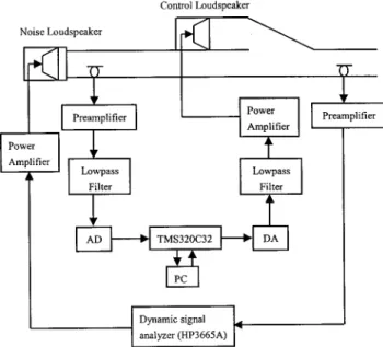
In ANC applications to date, feedforward control has been a most effective approach. However, a nonacoustical reference required by feedforward control is usually unavail-able in many applications. The spatially feedforward control structure shown in Fig. 1 appears to be a more viable ap-proach in dealing with such situations, especially when broadband attenuation is sought. The term, spatially feedfor-ward structure, stems from the fact that the ANC system in Fig. 1 includes an acoustic feedback path and is thus not a purely feedforward structure. In this case, stability and ro-bustness problems will arise and the achievable performance will also be degraded. For the spatially feedforward struc-ture, the zero spillover controller8 or the Roure’s controller9 can be used. However, these controllers may be noncausal
and require special modifications, e.g., direct truncation of impulse response, before practical implementation. There-fore, an optimization method combining an H2 performance objective with an H⬁constraint is proposed for the design of a spatially feedforward controller for duct. Using this ap-proach, nominal performance can be achieved under the H⬁ constraint of robust stability.
Much work has been addressed in the literature10–15on the mixed H2/H⬁ control. The controllers can be synthe-sized by the Riccati equation approach, the convex optimi-zation approach or the dynamic game approach, etc. In Ref. 15, a duct ANC system was developed using mixed H2/H⬁ control. The work incorporated an H⬁-constrained, LQG feedback controller with an internal model to attenuate a narrow-band disturbance. The controller is synthesized ana-lytically by solving the Riccati equations. In contrast to their approach, a numerical optimization approach, convex pro-gramming, applied within a general framework originally suggested by Boyd16is employed in this paper for achieving broadband noise reduction in a spatially feedforward struc-ture. Then, Q-parametrization17,18 is used to formulate all stabilizing controllers. The resulting Q-parametrization rep-resented by a finite impulse response 共FIR兲 filter transforms the design problem into a convex optimization problem in frequency domain. The approach suggested by Boyd16 is used in this work, where the optimal controller is found us-ing sequential quadratic programmus-ing.19,20Common causes of plant uncertainties are modeling errors, measurement noises, and the perturbations in physical conditions. A com-prehensive investigation on the effect of different physical conditions on ducts such as flow, temperature, lining, and radiation impedance, can be found in Ref. 21. However, in this paper, we shall focus on primarily the uncertainty result-ing from modelresult-ing error on which the robust stability con-straint is based.
This paper is organized as follows. First, the convex programming and Q-parametrization are presented in the
context of performance and robustness analysis. Then, the calculated controller is implemented as a FIR filter on a TMS320C32 digital signal processor共DSP兲. Finally, the pro-posed ANC system will be justified by experimental investi-gations and the results will be discussed.
II. ZERO SPILLOVER CONTROLLER AND ROURE’S CONTROLLER
Consider a standard control framework, with K the feed-forward controller, G the plant, w the exogenous input, z the controlled variables, u the control force, and y the measure-ment as illustrated in Fig. 2. Thus, the general input–output relation of the augmented plant can be expressed as follows:
冋
z共k兲 y共k兲册
⫽冋
Gzw共z兲Gzu共z兲 Gy w共z兲Gy u共z兲册冋
w共k兲 u共k兲册
, 共1兲where Gy u(z), Gzu(z), Gzw(z), and Gy w(z) are properly partitioned transfer matrices of G. They are represented in Figs. 3共a兲–共d兲. The closed loop transfer function can be ex-pressed as Tzw共z兲⫽关Gzw共z兲⫺„Gzw共z兲Gy u共z兲 ⫺Gzu共z兲Gy w共z兲…K共z兲兴关1⫺Gy u共z兲K共z兲兴⫺1 ⫽F共z兲S0共z兲, 共2兲 where F共z兲⬅Gzw共z兲⫺关Gzw共z兲Gy u共z兲⫺Gzu共z兲Gy w共z兲兴K共z兲 共3兲 is the spillover function and
S0共z兲⬅关1⫺Gy u共z兲K共z兲兴⫺1 共4兲
is the sensitivity function.
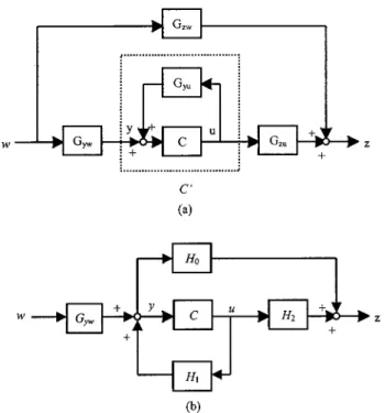
The block diagram of the duct system of Fig. 1 is shown in Fig. 4共a兲, using the notations of Eq. 共1兲. In terms of fre-quency response functions, letting the spillover function rep-resented in Eq. 共3兲 be zero leads to the so-called zero spill-over controller:8
KZS P共ej兲⫽
Gzw共ej兲
Gzw共ej兲Gy u共ej兲⫺Gzu共ej兲Gy w共ej兲 , 共5兲 where the digital frequency⫽⍀T with ⍀ being the analog frequency and T the sampling interval. On the other hand, the Roure’s controller that is equivalent to the zero spillover controller can be obtained by dividing the numerator and the denominator of Eq. 共5兲 by Gy w(ej):
KZS P共ej兲⫽
⫺Gzw共ej兲/Gy w共ej兲
Gzu共ej兲⫺Gy u共ej兲Gzw共ej兲/Gy w共ej兲
⫽ ⫺H0共ej兲
H2共ej兲⫺H1共ej兲H0共ej兲
⬅KRoure共ej兲, 共6兲
where H0(ej)⬅Gzw(ej)/Gy w(ej) is the frequency re-sponse function between the performance microphone and the measurement microphone, H1(ej)⬅Gy u(ej) is the fre-quency response function between the measurement micro-phone and the control speaker, and H2(ej)⬅Gzu(ej) is the frequency response function between the performance micro-phone and the control speaker. The block diagram of the Roure’s controller is shown in Fig. 4共b兲.
It is noted that in the Roure’s controller the frequency response function H0(ej) can be directly measured without knowing the disturbance w. The impulse response of the Roure’s controller is then obtained by inverse Fourier trans-form of KRoure(ej). However, this procedure generally re-sults in noncausal filters. Roure adopted a simple but effec-tive approach to overcome this difficulty. He chose to truncate the noncausal part directly and implemented the controller with a FIR filter.
III. DESIGN OBJECTIVE AND CONSTRAINT
The aforementioned Roure’s method provides a straight-forward means to obtain an implementable 共proper, stable, and causal兲 controller. Unlike Roure’s approach that requires the closed loop transfer function Tzw(z) be strictly zero, we seek to recast the problem into an optimization problem: find an implementable controller such that the following cost function of performance,
储Tzw共z兲W1共z兲储2
2, 共7兲
FIG. 1. Experimental setup of the ANC problem.
is minimized, where 储Tzw共z兲储2,
冉
1 2冕
⫺ 兩Tzw共ej兲兩2d冊
1/2 共8兲 represents the two-norm22 in discrete-time domain and W1(z) is a weighting function that is generally a low-pass function.In addition to performance consideration, robust stability is another important issue. Robust stability is understood as the robustness of stability of the closed loop ANC system against plant uncertainties and perturbations frequently en-countered in practical applications. One way of coping with system uncertainties and perturbations is to use an adaptive controller, whereas this paper adopted an alternative strategy—a robust controller which requires simpler imple-mentation than the adaptive counterpart. To this end, a robust stability constraint is incorporated into the aforementioned optimization problem. Assume the following perturbed plant model,23
Gp共z兲⫽Gy u共z兲关1⫹⌬共z兲兴, 共9兲
where Gy u(z) is the nominal plant,⌬(z) is the multiplicative uncertainty, and Gp represents the physical plant. The uncer-tainty ⌬(z) is assumed to be bounded by 兩⌬(z)兩⬍W2(z). The uncertainty considered here is primarily the difference between the plant model and the real plant beyond the con-trol bandwidth, which may cause excessive concon-trol output at high frequency. Therefore, it is important for the controller to be robust against this type of uncertainty. It can be shown by small-gain theorem that the condition of robust stability takes the form
储T0共z兲W2共z兲储⬁⬍1, 共10兲
where T0(z)⫽1⫺S0(z) is the complementary sensitivity function 关S0(z) is as defined in Eq. 共4兲兴 and W2(z) is a weighting function that is generally a high-pass function to be determined from the plant uncertainty.
In summary, the ANC problem can be written in the language of optimization as follows:
min K
储Tzw共z兲W1共z兲储2
2 共11兲
subject to
FIG. 3. The frequency responses of the nominal duct system.共a兲 The frequency response of Gy u; 共b兲 the frequency response of Gzu; 共c兲 the frequency response of Gzw; and共d兲 the frequency response of Gy w.
储T0共z兲W2共z兲储⬁⬍1. 共12兲 The control problem described in Eqs. 共11兲 and 共12兲 is a mixed norm problem that can be solved by a convex pro-gramming technique to be presented in the next section.
IV. CONVEX PROGRAMMING USING Q-PARAMETRIZATION
In this section, the formulation in Eqs.共11兲 and 共12兲 will be converted to a convex programming problem and solved by using a technique originally suggested by Boyd.16 The key step of the conversion to a convex problem is the so-called Q-parametrization17 to Youla’s parametrization.18 As-sume that the plant Gy u is stable. According to the method, the controllers that stabilize the closed loop system can be parametrized by a proper and stable transfer function Q(z) as follows:
K共z兲⫽ ⫺Q共z兲
1⫺Q共z兲Gy u共z兲
. 共13兲
The block diagram is shown in Fig. 5共a兲. More precisely, the resulting closed loop system will guarantee to be stable if the controller is selected in the form of Eq. 共13兲 with a proper and stable Q(z). The latter requirement is easily achieved in discrete time domain by choosing Q(z) to be a FIR filter. In addition, the controller design in Eq. 共13兲 is also known as the internal model controller because it has a ‘‘built in’’ nominal plant model Gy u.
At this point, the optimization problem has been formu-lated in frequency domain via Q-parametrization. To solve the problem, an approach proposed by Boyd and Helton24 was employed in the paper. The same method was also suc-cessfully used by Rafaely25 and Elliott who have done pio-neering work to solve an ANC problem for a headrest. This method first discretizes the frequency response function by uniformly sampling the unit circle, and then solves the opti-mization problem by convex programming.
Substituting Eq.共13兲 into Eqs. 共11兲 and 共12兲, Tzw(z) and T0(z) can be parametrized in terms of a proper and stable function Q(z):
Tzw共z兲⫽Gzw共z兲⫺Q共z兲Gy w共z兲Gzu共z兲,
T0共z兲⫽Q共z兲Gy u共z兲.
Thus minimization of 储Tzw储2 is tantamount to a model matching problem depicted in Fig. 5共b兲. Note that both Tzw(z)and T0(z) are affine functions of Q(z). By frequency discretization, the cost function and constraint function of the optimization problem now take the following form:
min q 1 N k
兺
⫽0 N⫺1 兩关Gzw共k兲⫺Q共k兲Gy w共k兲Gzu共k兲兴W1共k兲兩 2 共14兲 subject to 兩Q共k兲Gy u共k兲W2共k兲兩⬍1, k⫽0,1,...,N⫺1, 共15兲 where q⫽(q0q1•••qm⫺1)Tbeing the coefficient vector of the FIR filter Q with length m are the design variables and N is the number of frequency samples. Only the acoustic feed-back path Gy u(k) has to do with robust stability constraints. It should be noted that those gains of the transfer functions such as Gy u(z), Gzw(z), Gy u(z), and Gzu(z) are assumed to be time invariant for our application where the temperature is not changed much. To summarize, the optimization in Eq. 共15兲 is comprised of the design variable q, the cost function in quadratic form, and the constraint function in linear in-equality form.Define the following Hessian matrix26 FIG. 4. Two equivalent spatially feedforward controllers.共a兲 Block diagram
of zero spillover controller;共b兲 block diagram of the Roure’s controller.
FIG. 5. Block diagrams of Q-parametrization.共a兲 The internal model con-troller;共b兲 the model matching problem obtained from Q-parametrization.
Hs⫽
冤
2f x12 2f x1x2 ¯ 2f x1xn 2f x2x1 2f x22 ¯ 2f x2xn ] ] ] 2f xnx1 2f xnx2 ¯ 2f xn2冥
. 共16兲Because the Hessian matrix of the function in Eq. 共14兲 is positive definite, the function is a strictly convex function.26 Furthermore, the design specification in Eq.共15兲 is a convex specification because it is norm-bounded.27 Since the cost function and the constraint function are both convex, Eqs. 共14兲 and 共15兲 represent a convex problem. A local minimum of a convex problem is also a global minimum.
The method used in this work to compute the optimal controller by solving the optimization problem in Eqs. 共14兲 and 共15兲 was sequential quadratic programming26 which is provided as a MATLAB command constr in optimization toolbox. However, other programming methods such as semidefinite programming27 can be used. Because the func-tion constr was based on the sequential programming that accepts only linear constraints, the single robust stability constraint in Eq. 共12兲 has been replaced with N linear in-equality constraints in Eq.共15兲.
V. CONTROLLER IMPLEMENTATION AND EXPERIMENTAL INVESTIGATION
A duct made of plywood shown in Fig. 1 is used for verifying the proposed ANC method. The length of the duct is 440 cm and the cross section is 25⫻25 cm2. There is 10 cm between the primary source speaker and the measurement microphone. To reduce the undesirable acoustic feedback, we use the backward control loudspeaker facing the open end of the duct. The distance between the measurement microphone and the control speaker is 235 cm to ensure causality of the controller. The distance between the control speaker and the performance microphone is 110 cm. A floating point DSP, TMS320C32 equipped with four 16-bit analog IO channels, is utilized to implement the controller. The sampling quency is chosen to be 2 kHz. Considering the cutoff fre-quency of the duct 共approximately 700 Hz兲 and the poor response of speaker at low frequency, we chose control band-width from 200 to 600 Hz. It should be noted that a loud-speaker should be mounted near the primary noise source for identification of the frequency response functions Gy w(ej) and Gzw(ej) because the noise source共a fan, for example兲 is generally unmeasurable in practice.
A digital spatially feedforward controller is designed to reject the noise in the duct. The ANC system is as shown in Fig. 1. Figure 3共a兲 shows the measured frequency response function Gy u(ej). To weight performance as in Eq.共14兲, the weighting function W1(z) is chosen as a low-pass filter with cutoff frequency 600 Hz and unity gain, as shown in Fig. 6共a兲.
To weigh the robust stability as in Eq.共15兲, on the other hand, the weighting function W2(z) is determined from the
uncertainty definition in Eq 共9兲. The frequency responses of the nominal plant in 0– 800 Hz and in 0–1600 Hz are mea-sured. The former is taken as the nominal plant, while the latter the actual plant. By using the MATLAB command in-vfreqz, transfer functions of the nominal and true plant are calculated. Then the weighting function W2(z) is selected according to the following equation:
冏
Gp共ej兲 Gy u共ej兲⫺1
冏
⭐兩W2共ej兲兩 ᭙, 共17兲where Gp(ej) is the frequency response function of the actual plant and Gy u(ej) is the frequency response function of the nominal plant. Figure 6共b兲 shows the calculated uncer-tainty bounded by the weighting function W2whch is a high-pass filter with gain 2.5 and cutoff frequency 200 Hz.
The optimization problem formulated in Eqs. 共14兲 and 共15兲 with the design variables q of 128 coefficients 共initially set to be zeros兲 was solved numerically by using the MAT-LAB function constr. The unit circle was uniformly sampled at 2048 points. For the control bandwidth 200– 600 Hz, only 801 constraints need to be considered. In the choice of pa-rameters, sufficiently large number of frequency samples28N and long FIR filter Q are generally required to ensure an FIG. 6. Two weighting functions used in the implementation. 共a兲 The weighting function W1;共b兲 , the weighting function W2; , the uncertainty of the nominal plant.
accurate discrete approximation of the continuous problem. Titterton and Olkin29 suggested increasing the length of q and the length of N until the impulse response of q suffi-ciently decays such that any further increase of length would not result in significant improvement.
Figure 7共a兲 shows the coefficient vector of the control filter q with 128 coefficients. As can be seen in the figure, the impulse response decays almost completely. Any further in-crease in filter length will not provide significant improve-ment. The calculated coefficient vector q is then substituted into Eq. 共13兲 to obtain the optimal controller that is in turn converted to a FIR filter of length 256. Figure 7共b兲 shows the calculated impulse response of the controller. The resulting controller is then implemented on the platform of the DSP. An experiment is undertaken to verify the ANC system. The
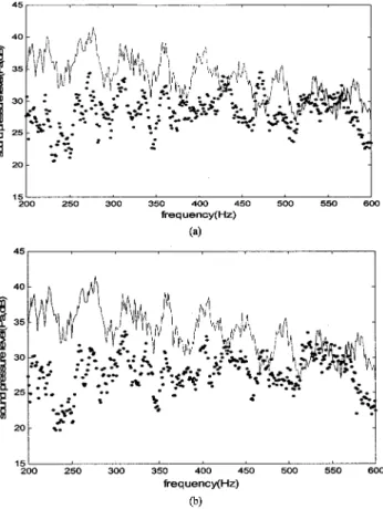
result of control in terms of pressure spectra measured at the performance microphone is shown in Fig. 8共b兲. The total attenuation within the control bandwidth is 5.9 dB.
Roure’s controller is also implemented for comparison with the mixed norm controller. Roure’s controller is calcu-lated from Eq. 共6兲, based on the measurable frequency re-sponse functions H0(ej), H1(ej), and H2(ej). The im-pulse response of Roure’s controller is shown in Fig. 7共c兲. Using Roure’s controller, the experimental result is shown in Fig. 8共a兲 with a total attenuation 5.4 dB. Detailed compari-son between the mixed norma controller and Roure’s con-troller is summarized in Table I.
VI. CONCLUSIONS
This paper presents a spatially feedforward design for active control of noise in a duct. As opposed to earlier meth-ods that compute optimal controllers analytically, this method utilizes a frequency domain convex programming technique. This approach is effective in that it guarantees to FIG. 7. The calculation result of Q-parametrization and the impulse
re-sponses of convex programming controller and Roure’s controller.共a兲 The coefficient vector q;共b兲 the impulse response of the convex programming controller; and共c兲 the impulse response of Roure’s controller.
FIG. 8. Active control results of the feedforward controllers.共a兲 Noise re-duction using Roure’s controller;共b兲 noise reduction using the convex pro-gramming controller. , control off;• • • •, control on.
TABLE I. Comparison of ANC methods.
Items Roure’s controller Convex programming controller Control bandwidth 200– 600 Hz 200– 600 Hz
FIR filter length 256 256
Maximal attenuation 15.5 dB 16.5 dB Total band attenuation 5.4 dB 5.9 dB
find the global minimum solution. In comparison to conven-tional LQG or H⬁ design, where experience is required for choosing appropriate weighting functions, all the functions required in our method can be derived directly from mea-sured data. The convex programming method, in conjunction with Q-parametrization and frequency discretization, proved to be useful in ANC application for several reasons. First, the chosen uncertainty model derived from measured data was found to be a reasonable model for construction of con-straints in optimization. This is an advantage over other ‘‘trial and error’’ design methods such as LQG in which we are unable to determine explicitly the weighting functions from measured data. Second, the design problem is a convex problem whose solution can easily be found using commer-cially available software such as MATLAB optimization toolbox. Third, optimization can be focused on performance since closed-loop stability has already been ensured by Q-parametrization.
To summarize, this research has two potential contribu-tions to the area of ANC. First, we have shown that the controller obtained from convex programming approximates well the idea spatially feedforward controller. It yields com-parable performance as the zero spillover controller and the Roure controller which use a direct truncation of the non-causal impulse response of the ideal controller. The proposed approach achieves nominal performance subject to the H⬁-constraint on closed-loop robust stability. Second, the procedures involved in the analysis and implementation phases are presented in detail. Experimental verifications of the proposed ANC system were conducted for a duct prob-lem. In particular, technical issues such as how to choose the plant uncertainty model and the performance index are ad-dressed.
ACKNOWLEDGMENTS
The work was supported by the National Science Coun-cil in Taiwan, Republic of China, under Project No. NSC 87-2212-E009-022.
1J. Hong, J. C. Akers, R. Venugopal, M. N. Lee, A. G. Sparks, P. D.
Washabaugh, and D. S. Bernstein, ‘‘Modeling, identification, and feed-back control of noise in an acoustic duct,’’ IEEE Trans. Control Syst. Technol. 4, 283–291共1996兲.
2Z. Wu, V. K. Varadan, and V. V. Varadan, ‘‘Time-domain analysis and
synthesis of active noise control systems in ducts,’’ J. Acoust. Soc. Am.
101, 1502–1511共1997兲.
3J. C. Carmona and V. M. Alvarado, ‘‘Active noise control of a duct using
robust control theory,’’ IEEE Trans. Control Syst. Technol. 8, 930–938
共2000兲.
4M. R. Bai and T. Y. Wu, ‘‘Study of the acoustic feedback problem of
active noise control by using the l1 and l2 vector space optimization
approaches,’’ J. Acoust. Soc. Am. 102, 1004 –1012共1997兲.
5M. R. Bai and H. P. Chen, ‘‘Development of a feedforward active noise
control system by using the H2 and H⬁ model matching principle,’’ J.
Sound Vib. 201, 189–204共1997兲.
6M. R. Bai and T. Y. Wu, ‘‘Simulation of an internal model-based active
noise control system for suppressing periodic disturbances,’’ ASME J. Vibr. Acoust. 120, 111–116共1998兲.
7M. R. Bai and H. H. Lin, ‘‘Comparison of active noise control structures
in the presence of acoustical feedback by using the H⬁ synthesis tech-nique,’’ J. Sound Vib. 206, 453– 471共1997兲.
8J. Hong and D. S. Bernstein, ‘‘Bode Integral Constraints, Colocation, and
Spillover in Active Noise and Vibration Control,’’ IEEE Trans. Control Syst. Technol. 6, 111–120共1998兲.
9
A. Roure, ‘‘Self-adaptive Broadband Active Sound Control System,’’ J. Sound Vib. 101, 429– 441共1985兲.
10D. S. Bernstein and W. M. Haddad, ‘‘LQG control with an H
⬁
perfor-mance bound: A Riccati equation approach,’’ IEEE Trans. Autom. Control
34, 293–305共1989兲.
11P. P. Khargonekar and M. A. Rotea, ‘‘Mixed H
2/H⬁ control: A convex
optimization approach,’’ IEEE Trans. Autom. Control 36, 824 – 837
共1991兲.
12C. W. Scherer, ‘‘Multiobjective H
2/H⬁ control,’’ IEEE Trans. Autom.
Control 40, 1050–1062共1995兲.
13Y. Theodor and U. Shaked, ‘‘Output-feedback mixed H
2/H⬁ control-A
dynamic game approach,’’ Int. J. Control 64共2兲, 263–279 共1996兲.
14
C. W. Scherer, ‘‘Mixed H2/H⬁ control,’’ in Proc. European Contr. Conf.
共ECC95兲 共1995兲, pp. 173–216.
15
J. Y. Lin and Z. L. Luo, ‘‘Internal model-based LQG/H⬁design of robust active noise controllers for acoustic duct system,’’ IEEE Trans. Control Syst. Technol. 8, 864 – 872共2000兲.
16
P. B. Boyd, V. Balakrishnan, C. H. Barrat, N. M. Khraishi, X. Li, D. G. Meryer, and S. Norman, ‘‘A new CAD method and associated architec-tures for linear controllers,’’ IEEE Trans. Autom. Control 33, 268 –283
共1988兲.
17D. C. Youla, J. J. Bongiorno, and H. A. Jabr, ‘‘Modern Wiener-Hopf
design of optimal controllers. Part I: The single-input-output case,’’ IEEE Trans. Autom. Control 21, 3–13共1976兲.
18M. Morari and E. Zafiriou, Robust Process Control共Prentice-Hall,
Engle-wood Cliffs, NJ, 1989兲.
19E. Gill, W. Murray, and M. H. Wright, Practical Optimization共Academic,
New York, 1981兲.
20
A. Grace, Matlab Optimization Toolbox, The Math Works, Inc.共1995兲.
21M. R. Bai and H. H. Lin, ‘‘Plant uncertainty analysis in a duct active noise
control problem by using the H⬁theory,’’ J. Acoust. Soc. Am. 104, 237– 247共1998兲.
22P. A. Nelson and S. J. Elliott, Active Control of Sound共Academic, London,
1992兲.
23J. C. Doyle, B. A. Francis, and A. R. Tannenbaum, Feedback Control
Theory共MacMillan, New York, 1992兲.
24
J. W. Helton and A. Sideris, ‘‘Frequency response algorithms for H⬁ op-timization with time domain constraints,’’ IEEE Trans. Autom. Control 34, 427– 434共1989兲.
25
B. Rafaely and S. J. Elliott, ‘‘H2/H⬁output feedback design for active
control,’’ ISVR, Univ. Southhampton, U.K., Tech. Memo 800共July 1996兲.
26
J. S. Arora, Introduction to Optimum Design共McGraw–Hill, New York, 1989兲.
27S. Boyd, L. Vandenberghe, and M. Grant, ‘‘Efficient convex optimization
for engineering design,’’ in Proc. IFAC Symp. Robust Contr. Design, Rio de Janeiro, Brazil共Sept. 1994兲
28
B. Rafaely and S. J. Elliott, ‘‘ H2/H⬁active control of sound in a headset:
Design and implementation,’’ IEEE Trans. Control Syst. Technol. 7, 79– 84共1999兲.
29
P. J. Titterton and J. A. Olkin, ‘‘A practical method for constrained opti-mization controller design: H2 or H⬁ optimization with multiple H2
and/or H⬁constraints,’’ in Proc. 29th IEEE Asilomar Conf. Signals, Syst., Comput.共1995兲, pp. 1265–1269.