The detection of dominant points on digital curves by scale-space filtering

(1)

Pattern Recoonition, Vol. 25, No. 11, pp. 1307-1314, 1992

Printed in Great Britain 0031-3203/92 $5.00+.00 Pergamon Press Ltd

THE D E T E C T I O N O F D O M I N A N T POINTS O N DIGITAL

CURVES BY SCALE-SPACE F I L T E R I N G

ZoO-CHANG PE! and CHAO-NAN LIN

Department of Electrical Engineering, National Taiwan University, Taipei, Taiwan, Republic of China (Received 15 June 1991; in revised form 4 December 1991; received for publication 16 March 1992) Abstract--The detection of dominant points is an important preprocessing step for shape recognition. An effective method of scale-space filtering with a Gaussian kernel is introduced to detect dominant points on digital curves. The conventional polygonal approximation algorithms are time-consuming and need input parameter tuning for Gaussian smoothing the noise and quantization error, also they are sensitive to scaling and rotation of the object curve. The above dit~culty can be overcome by finding out the dominant points at each scale by scale-space filtering. By tracing back the dominant point contours in the scale-space image, the stable cardinal curvature points can be detected very accurately. This new method requires no input parameters, and the resultant dominant points do not change under translation, rotation and scaling. Meanwhile a fast convolution algorithm is proposed to detect the dominant points at each scale.

Dominant points Scale-space Gaussian smoothing Curvature

I. I N T R O D U C T I O N

Various representations of two-dimensional shape have been developed in the computational vision literature. (11 It has been suggested from the viewpoint of the human visual system that the dominant points having high curvature are sufficient to characterize the shape of the object. In general, the current existing methods for detecting dominant points are divided into two major groups: one is to detect the dominant points directly through angle or corner detection schemes, (2-7~ and the other is to obtain a piecewise linear polygonal approximation of the digital curve subject to a certain constraint on the goodness of fit.(s-101

The recent Teh-Chin algorithm (7) is a good example of detecting dominant points based on angle detection. The algorithm does not require input parameters and works well on an object curve which is not corrupted with noise. However, it is very sensitive to noise, some false dominant points will be detected due to quantization error and noise effect. On the other hand, the curvature guided polygonal approximation method (1°~ makes use of Gaussian smoothing to reduce the effect of noise, but it requires two input parameters, namely, the width of a Gaussian filter and the collinearity tolerance for doing a split-and-merge algorithm. There is a trade-off in seleoting the width of the Gaussian filter, a larger width will remove small details of the boundary curvature, a smaller width will permit false concavities and convexities. Recently, Ansari and Huang used the advantages of both approaches, they introduced a new method (~11 which was non-parametric with no input parameters and less sensitive to noise. However, this method requires the support region for each contour point to be determined, and then the contour is smoothed by an adaptive Gaussian

filter with a width proportional to the support region. This complicates the smoothing procedure a lot and increases the computational efforts and complexities. Mokhtarian and Mackworth "2~ have suggested a number of necessary criteria which any reliable method for curve representation and recognition must satisfy:

(11 The feature selection or extraction method must be computed efficiently.

(2) The extracted feature should be invariant under translation, rotation and scaling.

(3) The feature representation should contain information about the curve at varying levels of detail, and should uniquely specify a single curve.

In order to satisfy the above conditions, we introduce the scale-space filtering to find out the relevant dominant points at each scale. Scale-space filtering (~ 31 is a useful signal description method that deals gracefully with the problem about scales by treating the size parameter of the smoothing kernel as a continuous parameter. As the scale parameter is varied, the dominant points of each scale in the smoothed signal in general move continuously. By tracing back the dominant point contour in the scale-space image, we are able to detect the stable cardinal curvature points very accurately. They are extreme curvature points of the digital curve that are stable with respect to Gaussian smoothing for a reasonable wide range of Gaussian filter width, and can represent a unique shape attribute of the curve. Also the resultant dominant points are shown to be invariant under translation, rotation and scaling. Meanwhile a fast convolution algorithm is proposed to extract the dominant points at each scale very efficiently.

The arrangement of this paper is organized as follows. In Section 2, we introduce how to detect the dominant points at each scale by scale-space filtering.

(2)

1308 S.-C. PEI and C.-N. LItq

In Section 3, we explain how to correct the moved dominant points on each scale into the right locations by tracing back the scale-space image. Section 4 de- scribes how to determine an appropriate scale to find out the stable cardinal curvature points accurately. Also a fast convolution algorithm is introduced in Section 5 to compute the derivative of curvature efficiently. Finally conclusions are made in Section 6.

2. DETECTION OF DOMINANT POINTS BY SCALE-SPACE FILTERING

Points with high curvature along a shape contour are rich in information content and are sufficient to characterize the object contour. We call these points the dominant points. In this section, the curvature computation and the dominant point detection will be described in detail.

2.1. Curvature computation on a curve

Consider a path length variable t along the curve C and express the curve in terms of two functions x(t)

and y(t)

C = {x(t),y(t)} (l)

where t is the path length of the curve, x(t) the x-coordinate of the curve at path length t, and y(t) the y-coordinate of the curve at path length t. Let K be the curvature of a planar curve at a point p which is defined as the instantaneous rate of change of the slope angle of the tangent at point p with respect to length t

dO

K = - - . (2)

dt

K can be computed if the curve is expressed in terms of the derivatives of functions x(t) and y(t). Define

, dy y , , d2y (3)

Y = dx' dx 2" It is known that

y l /

K - (1 + (y,)2)3/2' (4)

Since the curve is a function of path length t, the above

y' and

y"

can be expressed in terms of the first and

second derivatives of x(t) and y(t). Denote

dx d2x dy d2y ~ = d t t ' ~ = d t 2' Y = d t ' J > = d ~ ' (5) Then and f y ' = ± , y " = (6) x .~3 K - (~2 + 3)2)3/2" (7)

2.2. Finding out the relevant dominant points by scale- space filtering

Scale-space filtering is useful to describe a signal qualitatively. (la) A unified and organized description can be produced by treating each contour in the scale-space image as a single physical event, observed through a continuum of Gaussian smoothing filters, rather than as a set of unrelated events. Hence we can find out the relevant dominant points from the contour in the scale-space image. In this section, we introduce how to derive a scale-space image from a shape and how to find out the dominant points from the scale- space image.

Let g(t, a) be the Gaussian kernel 1

_ e-t2/2o ~

oct, ,~) - ~

(8)

where t is the path length of the shape contour and ~r the filter width (spatial support) of the Gaussian kernel. By changing the value of a, we can get the Gaussian kernel at various scales.

In order to reduce the quantization error and noise in computing the curvature of the digital curve, the digital curve is first smoothed by the Gaussian filter with small scale a, i.e.

co 1 ~ x(z)e_o_o2/2O2dz x(t) = x(t).g(t, (r) =/12rrt# x / x J v l oo (9a) 1 co

y(t) = y(t) • g(t, o-) - v,-,/197r~tr -:o ~ y('r) e - t t - ,)2/2o2 dz (9b) where * is the convolution operation and a = 2 pixeis is used in our paper. By equation (7), the curvature of the contour can be evaluated by using the above smoothed x(t) and y(t)

K(t) - (~2 + ~2)3/2' (10)

The curvature of the contour at various scales is computed by convolving K(t) with a one-dimensional kernel g(t, tr)

co

1 ~

K(z)e_(t_,)2/2O~d~

K i t , ~r) = K ( t ) * g ( t , ~r) - x / ( 2 ~ ) ~ -co

(11) where K(t, tr) is the curvature at scale a. Since the dominant points are located at the extreme of curvature which is equivalent to the zero-crossing of the derivative of the curvature

li:(t, ~) - dK(t, ~) (12)

dt

Equations ( l l ) and (12) are combined to reduce the quantization error

l ( ( t , ~ r ) = d {K(t)*g(t, cr)} = K(t)* dg(t'a) (13) dt

(3)

T h e d e t e c t i o n of d o m i n a n t p o i n t s o n d i g i t a l c u r v e s by scale-space filtering 1309

Fig. 1. Original curve of a wire cutter.

( o ) G = 3 ( b ) i f = 1 9

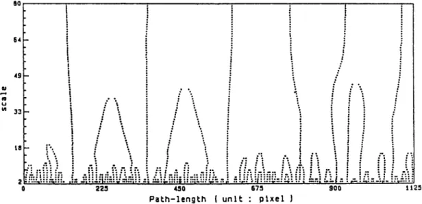
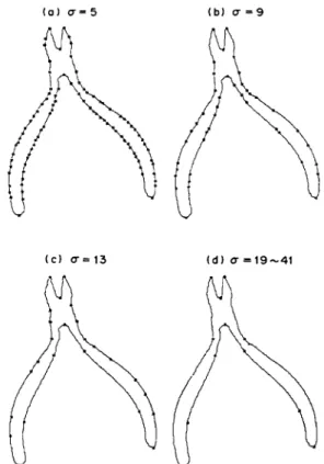
Then we can find the d o m i n a n t points at each scale. Figure 1 shows the original c o n t o u r of a wire cutter. As the scale parameter tr is varied and increased by a small amount, the extrema or zero-crossing in the smoothed curvature a n d its derivatives in general move continuously. The behavior of extrema over scale is characterized in terms of the scale-space image as shown in Fig. 2. The scale-space images contain several contours which are closed at the top a n d open at the bottom, now extrema points are created at higher levels of detail (more smoothing). O n e can track back the extreme points at lower levels in the neighborhood of the previous ones at higher levels. The positions of d o m i n a n t points on the c o n t o u r at various scales are illustrated in Figs 3(a)-(d). In the next section, we will describe how to combine various levels of information in the scale-space image in order to obtain a representation for the curve.

3. POSITION CORRECTION O F DOMINANT POINTS BY TRACING BACK ALONG SCALE-SPACE CONTOURS

F r o m Figs 3(a) to (d) notice that the locations of d o m i n a n t points will drift as the scale increases (see the top two sharp tips of the wire cutter in Fig. 3(c)).

( c ) ~ = 4 1 ( d ) ~ = 5 0

Fig. 3. The detected dominant points on the contour at various scales. Notice that the top two sharp tips in (c) drift

from the original positions very severely.

In order to correct the shifting, we must trace it back along the contour in the scale-s pace image, as shown in Fig. 4~a).

The location position of the d o m i n a n t points at smaller scale is much more accurate than the ones at larger scale. In this paper, we start the scale-space filtering from the scale tr = 3, and compute the curva-

O0 §4 t 49 . - , . . " '... i : ul 3 3 ~ • ~ ,' : " I : ! : ,. ) - ~ - .. ... • ! - . ~t;:.",".. '. l~," . ":" i'~ :. :'; ,~ ,".~; ,-. "" , ! : ; " ~ ' . ~ . ~ , , , " '~L '~, ,: ~ r . . :- i " "~:" '" -'~" 2 2 5 4'~0 6 7 5 9 0 0 t 1 2 5 P a L h - l e n g k h { u n i t : : p t x e l J

(4)

( b ) o " = 9

ture of various levels for the scales tr = 3, 5, 7, 9 , . . . , 79. Let array p3(0 record the root location of d o m i n a n t points at the smallest scale, array p2(i) the location of d o m i n a n t points at current tr, and array pl(i) the location of d o m i n a n t points at the preceding scale t r - 2. The tracing back step is done immediately following the detection of the d o m i n a n t points at each scale, this will correct the shifted d o m i n a n t points into the right position, the major algorithm is summarized as follows:

(1) Start at scale a = 3, find the d o m i n a n t points at the extreme of curvature K(t, 3), which are located at path length t = nl, n2,n3,... ,nM1. Then save them in array p3(i) and pl(i) for i = 1, 2 . . . M1.

(2) Increasing the filter width by 2, tr = tr + 2. Find the d o m i n a n t points at the extreme of curvature K(t, tr), which are located at path length t = ml, m 2 , . , m u 2 Then save them in array p2(i) for i = 1, 2 . . . M2. By the scale-space theory, (14) the n u m b e r of d o m i n a n t points is m o n o t o n o u s l y decreasing as the scale is increased, i.e. M2 < M1.

( c } o " = 1 3

Scale

Path-length

Fig. 4(a). Position correction of dominant points by tracing back along scale-space contours.

( o ) 0 - = , 5

1310 S.-C. 1~] and C.-N. LIN

( d ) o" = 1 9 ~ 4 1

Fig. 5. The detected dominant points on the curve at various scales are traced back into the right locations, as compared with Fig. 3. There are 12 stable extreme curvature dominant points detected in the range of Gaussian smoothing tr = 19-41. (3) Trace the shifted dominanl point location back to tr = 3 The algorithm is listed as follows:

F o r i = 1 to M2

search pl(k) so that Min Ipl(j) - p 2 ( i ) l ,

k f o r l < j < M 1 p3(i)=p3(k) 80 u I/I 64 49 3 3 18 • • • • ° ° • ° • • • • • ° • • • ° • • • ° • • ° . ° . ° • . . . ::" . : ' : : : ' . : 7 : . " . . . : : ' . : . . : .... : : 2 " ; : . . : : : . . : : : . : . z .::.Z.::::.::" ,:. ":::':i:----:; _7.;:: . ; "_:,::::~ ::.'.7_.'.: ~:-.. r :: :,:: : :i; ::::~-: "~: :: ; --'; " " i ,. : ,'-: :,:- ".~- ::~:'::: ~2S 45o 67,~ ~oo t t~

Pal:n-length

I uni~ : laixel I Fig. 4(b). Tracing back scale-space image of Fig. 2.

(5)

The detection of dominant points on digital curves by scale-space filtering 1311 end for (4) For i = 1 to M2 pl(i) = p2(i) end for go to step (2).

This tracing back algorithm is very simple and can be computed very efficiently. Figure 4(b) illustrates the tracing back scale-space image of Fig. 2. The dominant points detected on the curve at various scales are traced back into the right locations as shown in Figs 5(a)-(d). By comparison of Figs 3(c) and 5(d) with the same scale a = 41, the dominant points found by tracing back are more accurate. Also we notice that there are 12 extreme curvature dominant points in Fig. 5(d) that are stable with respect to Gaussian smoothing for a reasonable range of values oftr = 19-41. We shall refer to those stable local extreme curvature points as the cardinal curvature points. It°)

( 0 ) 0 " = 5

are stable with respect to a reasonable degree of scaling. The simplest method is that the number of dominant points is specified in advance. The scale is gradually increased until the number of dominant points at one scale is equal to the specified one. Another preferred method is that we terminate the algorithm when the number of dominant points does not change in a duration A , above some threshold. We modified step (4) of the above algorithm in Section 3 as

(4) If M1 = M2 then counter = counter + 1

If counter > threshold, find the cardinal dominant points.

else if counter < threshold, go to step (2). else if M1 # M2, then

counter = 0 M1 = M 2 go to step (2)

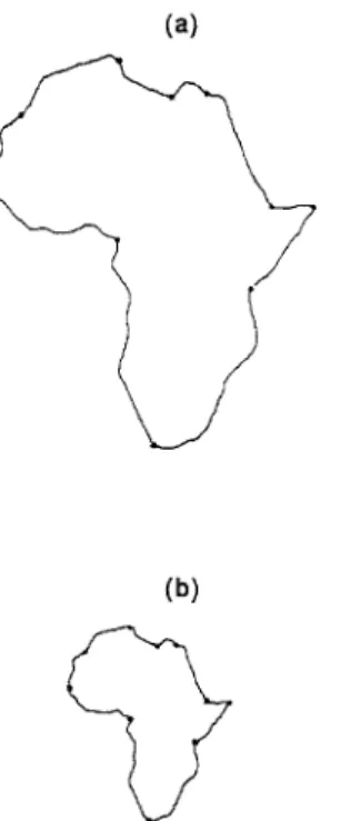
where the counter measures the duration Air where the number of dominant points does not change, i.e. M1 = M2, the typical threshold value is chosen from 6 to 8 in our computer simulations. Figures 6(a)-(d) show another more complex example of the Africa 4. T E R M I N A T I O N AT AN A P P R O P R I A T E SCALE VALUE

T O D E T E C T T H E C A R D I N A L C U R V A T U R E P O I N T S How to decide the scale value to terminate Gaussian smoothing? The resultant cardinal curvature points

( b ) O" = 13

( c ) O" = 1 9 ( d ) O" = 2 9 ~ 4 !

Fig. 6. The traced-back detected dominant points of the Africa curve at various scales, in which 10 cardinal curvature points in (d) are accurately detected and stable in the scale range from a = 29 to 41.

(6)

1312 S.-C. l~l and C.-N. LIN

curve in which 10 cardinal curvature points are accurately detected and stable in the range from a = 29 to 41.

5. FAST ALGORITHM

Chen et al. (15) proposed a fast algorithm for computing the convolution of an image with L O G (Laplacian of Gaussian) mask. They used a well-known property that a L O G of width cr can be decomposed as a Gaussian mask and a L O G of width a~ < a. Since the Gaussian kernel is neither time-limited nor band- limited, they must carefully establish effective, inde- pendent limits on the L O G and Gaussian mask required for proper performance." 6,17)

Here, we can derive a similar fast algorithm for computing the convolution of a curvature with the derivative of Gaussian kernels (see equation (13)). This fast technique is described in Section 5.1.

5.1. Fast convolution with the derivative of the Gaussian kernel

There is a special property about the Gaussian function as follows.

Theorem 1. The convolution of two Gaussian functions with width aa and a2 will produce another Gaussian function with width a = (a~ + 2 1/2 a2) . This means that

9(t,a) = g(t, ax)*O(t, a2), where a = ~/(a2x + a~).

(14)

By Theorem 1, we derive the convolution of the curvature with the derivative of the Gaussian kernel as follows:

a) = d {K(t)*9(t, a)} = d

/~(t,

~t {K(t)*O(t, aO*O(t, Aa)}

= K(t)*~tO(t, al) *O(t,A~)

with a = ~/(~2 _ a~). (15)

Thus, the derivative of curvature at current scale a can be computed efficiently by convolving the derivative of curvature at the preceding scale a l with a Gaussian kernel with width Aa. This can save a lot of derivative operations at each scale except at the smallest starting scale e = 3.

Since the Gaussian smoothing function is not time- limited, if we take the finite Gaussian filter length as [ - 3 a , 3 a ] , there must occur some truncation error. Also we sample the continuous Gaussian filter into a discrete Gaussian filter, since the Gaussian filter is not band-limited, this will cause some aliasing error during the sampling process. These aliasing and truncation errors will accumulate as this itcrativc convolution process goes on. In order to overcome this accumula- tion error effect, we adopt the sampling interval for the Gaussian kernel as 1 pixel for all scales, also the scale

interval A~r is switched from 2 to 4 pixels at large scales. This can reduce the aliasing error effectively. By equation (15), we summarize the fast algorithm as follows:

(1) By equation (13), start computing the derivative of curvature at the smallest scale cr 1 = 3, and denote it b y / ( ( t , tr~).

(2) Set the scale interval to 2 pixels, thus the next scale is a2 = trl + 2, then /~(t, az) can be computed simply by convolving K(t, tr 0 with the Gaussian kernel #(t, Aa), this means that

/~(t, a2) = I((t,

a,)9(t,*

Aa). (16) (3) Repeat step (2) until the scale a = 12.

(4) Reset the scale interval Aa to 4 pixels to reduce aliasing error. Repeat step (2) until the dominant points have been found.

Combining this fast method and the tracing-back algorithm, we can find the relevant dominant points rapidly.

In order to see that the detected dominant points by this approach are very stable and remain unchanged with respect to translation, rotation and scaling, we perform several experiments the results of which are shown in Figs 7 and 8. The detected dominant points of the original curves at normal scale are shown in Figs 7(a) and 8(a), respectively. Figures 7(b) and 8(b) show the results when the two curves are reduced by half, i.e. scaling = 0.5. The detected curve shown in

(a)

(b)

(c)

Fig. 7. The detected 12 dominant points by scale-space filtering are very stable and remained unchanged with respect to translation, rotation and scaling: (a) original curve; (b) • scaling = 0.5; (e) translation = (10, 10) pixels, scaling = 0.5

(7)

(a)

The detection of dominant points on digital curves by scale-space filtering 13 l 3

(b)

Fig. 8. Ten stable cardinal dominant points of the Africa curve are detected under (a) original scale and (b) half scale

at scaling = 0.5.

Fig. 7(c) is obtained if the wire cutter curve is translated, scaled and rotated under translation = (10, 10) pixels, scaling = 0.5 and rotation = 30 deg. Notice that the detected d o m i n a n t points by this approach remain very stable and do not change under translation, rotation and scaling. Hence the dominant points found by the scale-space algorithm satisfy M o k h t a r i a n and M a c k w o r t h ' s criteria "2~ discussed above for reliable recognition.

6. CONCLUSIONS

The information of a curve is concentrated and

characterized at the dominant points with high curvature. In this paper, we have introduced the method of scale-space filtering with a Gaussian kernel to effec- tively detect these cardinal curvature points on the

digital curve. These extracted features can uniquely specify a curve qualitatively.

The uniqueness of this m e t h o d is that the dominant points found remain very stable, and will not change as the curve translates, rotates and scales. Thus we can recognize shapes using the dominant points under distortion of translation, rotation and scaling.

Another advantage of finding d o m i n a n t points is

that it is very useful in the recognition of partial shapes.Ii 8,19)

REFERENCES

1. S. Marshall, Review of shape coding techniques, Image Vision Comput. 7, 281-294 (1989).

2. A. Rosenfeld and E. Johnston, Angle detection on digital curves, IEEE Trans. Comput. 22, 875-878 (1973). 3. A. Rosenfeld and J. S. Weseka, An improved method of

angle detection on digital curves, IEEE Trans. Comput. 24, 940-941 (1975).

4. H. Freeman and L. S. Davis, A corner-finding algorithm for chain coded curves, IEEE Trans. Comput, 26, 297-303 (1977).

5. P. V. Sankar and C. V. Sharma, A parallel procedure for the detection of dominant points on a digital curve, Comput. Graphics Image Process. 7, 403-412 (1978). 6. I. M. Anderson and J. C. Bezdek, Curvature and tangen-

tial deflection of discrete arcs: a theory based on the commutator of scatter matrix pairs and its application to vertex detection in planar shape data, IEEE Trans. Pattern Analysis Mach. Intell. PAMI-6, 27-40 (1984). 7. C. H. Teh and R. T. Chin, On the detection of dominant

points on digital curves, IEEE Trans. Pattern Analysis Mach. Intell. PAMI-II, 859-872 (1989).

8. T. Pavlidis, Algorithms for shape analysis and waveforms, IEEE Trans. Pattern Analysis Mach. lntell. PAMI-2, 301-312 (1980).

9. J.G. Dunham, Optimum uniform piecewise linear ap- proximation of planar curve, IEEE Trans. Pattern Analy- sis M ach. Intell. PAMI-8, 67-75 (1986).

10. N. Ansari and J. Delp, On detecting dominant points, Pattern Recognition 24, 441-451 (1991).

11. N. Ansari and K. W. Huang, Non-parametric dominant point detection, Pattern Recognition 24, 849-862 (1991). 12. F. Mokhtarian and A. Mackworth, Scale-based description and recognition of planar curves and two-dimen- sional shapes, I EE E Trans. Pattern Analysis Mach. Intell. PAMI-8, 34-43 (1986).

13. J. Babaud, A. P. Witkin and M. Baudin, Uniqueness of the Gaussian kernel for scale-space filtering, IEEE Trans. Pattern Analysis Mach. Intell. PAMI-8, 26-33 (1986). 14. A. L Yuille and T. A. Poggio, Scaling theorems for zero

crossing, IEEE Trans. Pattern Analysis Mach. Intell. PAMI-8, 15-25 (1986).

15. J. S. Chen, A. Huertas and G. Medioni, Fast convolution with Laplacian-of-Gaussian masks, I EEE Trans. Pattern Analysis Mach. Intell. PAMI-9, 584 590 (1987). 16. G.E. Sotax, Jr and K.L. Boyer, Comments on fast

convolution with Laplacian-of-Gaussian masks, IEEE Trans. Pattern Analysis Mach. Intell. PAMI-11, 1329- 1332 (1989).

17. G.E. Sotax, Jr and K.L. Boyer, The Laplacian-of- Gaussian kernel: a formal analysis and design procedure for fast, accurate convolution and full-frame output, Comput. Vision Graphics Image Process. 48, 147-189 (1989).

18. L. Gupta and K. Malakapalli, Robust partial shape classification using invariant breakpoints and dynamic alignment, Pattern Recognition 23, 1103-1111 (1990). 19. H. C. Lin and M. D. Srinath, Partial shape classification

using contour matching in distance transformation, IEEE Trans. Pattern Analysis Mach. Intell. PAMI-12, 1072- 1079 (1990).

About the Author--Soo-CHA~G PEl was born in Soo-Auo, Taiwan, Republic of China, on 20 February 1949.

He received the B.S. degree from National Taiwan University in 1970 and the M.S. and Ph.D. degrees from the University of California, Santa Barbara, in 1972 and 1975, respectively, all in electrical engineering. He

(8)

1314 S.-C. PEI and C.-N. LIN

was an engineering officer in the Chinese Navy Shipyard at Peng Fu Island from 1970 to 1971 and a Research Assistant at the University of California, Santa Barbara, from 1971 to 1975. He was Professor and Chairman in the Department of Electrical Engineering at Tatung Institute of Technology from 1981 to 1983. Presently, he is the professor of Department of Electrical Engineering at National Taiwan University. His research interests include digital signal processing, digital picture processing, optical information processing, laser and holography. Dr Pei is a member of the IEEE, Eta Kappa Nu and the Optical Society of America.

About the Author--O-L~o-NAN LIN was born in Taiwan, Republic of China, on 7 September 1966. He

received the B.S. degree from National Tsing Hua University, Hsinchu, in 1989 and the M.S. degree from National Taiwan University, Taipei, in 1991, both in electrical engineering. Presently, he is a communication officer in the Chinese Army. His research interests include digital signal processing, image processing and computer graphics.