混合型線性規劃的計算方法

行政院國家科學委員會補助專題研究計畫成果報告

※※※※※※※※※※※※※※※※※※※※※※※※

※ ※

※　　 混合型線性規劃的計算方法　 　　　　※

※　　　　　　　 　　※

※※※※※※※※※※※※※※※※※※※※※※※※

計畫類別：þ個別型計畫　　□整合型計畫

計畫編號：NSC－89－2213－E－004－004

執行期間：88 年 08 月 01 日至 89 年 07 月 31 日

計畫主持人：陸行

共同主持人：蔡瑞煌

本成果報告包括以下應繳交之附件：

□赴國外出差或研習心得報告一份

□赴大陸地區出差或研習心得報告一份

□出席國際學術會議心得報告及發表之論文各一份

□國際合作研究計畫國外研究報告書一份

執行單位：政治大學應用數學系

中　華　民　國　89　年　07　月　31　日

行政院國家科學委員會專題研究計畫成果報告

混合型線性規劃的計算方法

計畫編號：NSC 89-2213-E-004-004

執行期限：88 年 08 月 01 日至 89 年 07 月 31 日

主持人：陸行 政治大學應用數學系

共同主持人：蔡瑞煌 政治大學資訊管理學系

In this paper, we present an auxiliary algorithm that, in terms of the speed of obtaining the optimal solution, is effective in helping the simplex method for commencing a better initial basic feasible solution. The idea of choosing a direction towards an optimal point presented in this paper is new and easily implemented. From our experiments, the algorithm will release a corner point of the feasible region within few iterative steps, independently of the starting point. The computational results show that after the auxiliary algorithm is adopted as phase I process, the simplex method consistently reduce the number of required iterations by about 40%.

Keywords: Linear Programming,

Interior-point-based Solution. 中文摘要 在本篇報告中，我們以求解速度的角 度呈現一輔助的運算法則，幫助單體法從 較佳的初始可行解開始求解。從實驗當 中，選擇一新且易於執行的方向，且和起 始點無關，免除在遞迴步驟計算可行解區 域的角點的目標函數值。計算結果顯示， 採納在階段 I 使用輔助運算法則，在階段 II 使用單體法，則降低所需遞迴步驟約百分 之四十。 關鍵詞：線性規劃、內點解法。

2. The Proposed Approach

Consider the following standard form of LP problem (1). In (1), xt ≡ (x1 x2 ... xn), A~ is an m×n matrix, t b ~ ≡ (b1 ~ 2 b ~ _... m b ~ ), ~ct ≡ (c1 ~ 2 c ~ _... n c ~ _{), and 0 is denoted}

a column vector, of appropriate dimension, with each component equals zero.

Minimize z = ~ct

x

Subject to A~ x≥ b~ (1) x≥0

Let LP problem (2) be a normalization version of LP (1). That is, c ≡

c c ~ ~ , Ai_•≡ • • i i A A ~ ~ , and bi ≡ • i i A~ b ~ , whereAi_• ~ is the ith row vector of A~ and the Euclidean norm is adopted for ||⋅||. It is easy to check the sets of feasible solutions as well as the optimal solutions of both LP (1) and LP (2) are equivalent.

Minimize z = ctx

Subject to A x≥b (2) x≥0

Below, we take LP (2) as our standard form of input to illustrate the idea of the improving feasible direction in details.

h(k)≡ ∑ ∑ ∑ ∑ Ω ∈ Ω ∈ • Ω ∈ Ω ∈ • + + k k k k j j i t i j j i t i 2 1 2 1 e A e A (3) g(k) =       ≠ − − = c h c h c h c h 0 ) ( ) ( ) ( ) ( if if k k k k . (4)

    ≤ ≤ < − = , g 0, 1 n; g x min η ( ) ) ( ) ( (k) j k j k j k j    ≤ ≤ < − • • • _{, 0, 1 m} b () ) ( ) ( i k i k i k i i g A g A x A ₍₅₎

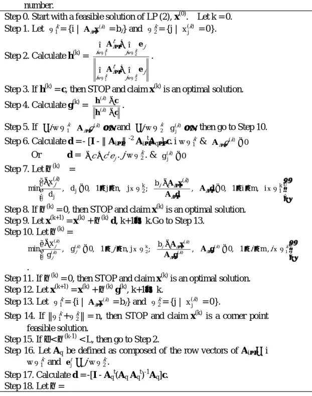
Table 1 displays the proposed algorithm. From Lemma 2, the criterion of h(k) = c in Step 3 is a sufficient stopping criterion of the proposed algorithm. Step 5 guarantees x(k+1)

is always a boundary point of P. Theorem 1 says that the criterion in Step 6 is also a sufficient stopping criterion of the proposed algorithm. As to find an initial feasible solution of LP(2) in Step 0, we can apply the same algorithm to LP (2) with artificial variables.

Table 1. The proposed algorithm. ej is an n-dimensional unit vector with 1 for its jth

component and 0 for the rest, and Ai_• is the ith row of A. ε < 10

-6

, and L is a large number.

Step 0. Start with a feasible solution of LP (2), x(0). Let k = 0. Step 1. Let k 1 Ω = {i | (k) i x A_• = bi} and Ωk2= {j | ) ( j x k = 0}. Step 2. Calculate h(k) = ∑ ∑ ∑ ∑ Ω ∈ Ω ∈ • Ω ∈ Ω ∈ • + + k k k k j j i t i j j i t i 2 1 2 1 e A e A .

Step 3. If h(k) = c, then STOP and claim x(k) is an optimal solution. Step 4. Calculate g(k) = c h c h − − ) ( ) ( k k . Step 5. If k i∈Ω₁ ∀ ( ) ≥0 • k i g A and k j∈Ω₂ ∀ g( ) 0 j ≥ k _{, then go to Step 10.}

Step 6. Calculate d = - [I -∥Ai•∥-2 Ai•tAq•] c. i ∈Ω1k & 0

) ( _< • k i g A Or d = t _j e c c+ − . j∈ k 2 Ω . & g(j) <0 k Step 7. Let η (k) =         Ω ∉ ≤ ≤ < − Ω ∉ ≤ ≤ < − • • • k 1 ) ( k 2 j j ) ( i m, i 1 , 0 , b ; j n, j 1 , 0 d , d x min A d d A x A i i k i i k j

Step 8. If η (k) = 0, then STOP and claim x(k) is an optimal solution. Step 9. Let x(k+1) = x(k) + η (k)d, k+1→k.Go to Step 13.

Step 10. Let η (k) =         Ω ∉ ≤ ≤ < − Ω ∉ ≤ ≤ < − • • • k k i k i k i i k j k j k j i i j 1 ) ( ) ( ) ( k 2 ) ( ) ( ) ( , m 1 , 0 , b ; j n, 1 , 0 g , g x min A g g A x A .

Step 11. If η (k) = 0, then STOP and claim x(k) is an optimal solution. Step 12. Let x(k+1) = x(k) + η (k)g(k), k+1→ k. Step 13. Let k 1 Ω = {i | (k) ix A_• = bi} and Ωk2= {j | ) ( j xk = 0}. Step 14. If || k 1 Ω + k 2

Ω || = n, then STOP and claim x(k) is a corner point feasible solution.

Step 15. If ε < η (k-1) < L, then go to Step 2.

Step 16. Let Aq be defined as composed of the row vectors of Ai• ∀ i ∈ k

1

Ω and t

j

e ∀j∈Ωk₂.

Step 17. Calculate d = -[I - Aqt(AqAqt)-1Aq]c.

        Ω ∉ ≤ ≤ < − Ω ∉ ≤ ≤ < − • • • k 1 ) ( k 2 j j ) ( i m, i 1 , 0 , b ; j n, j 1 , 0 d , d x min A d d A x A i i k i i k j Step 19. Let x(k+1) = x(k) + ηd, k+1→ k. Step 20. Let k 1 Ω = {i | (k) ix A_• = bi} and Ωk2= {j | ) ( j xk = 0}. Step 21. If || k 1 Ω + k 2

Ω || = n, then STOP and claim x(k) is a corner point feasible solution; else go to Step 16.

In order to avoid the zig-zag situation during the process, the loop of Steps 16-21 is set for determining a basic feasible solution to start the simplex method. Generally, Steps 16-21 implement the gradient projection method to obtain a corner point of feasible solution. The matrix

M ≡I - Aqt(AqAqt)-1Aq is the project matrix

corresponding to the boundary. Action by it on any vector yields the projection of that vector onto the boundary. Since d = -Mc in Step 17, d is a feasible direction of descent on the boundary if d ≠0. That is, we have ct x(k+1) < ctx(k), if x(k+1) (= x(k) + ηd) does not

equal x(k). Step 18 guarantees x(k+1) is always a boundary point. Before obtaining a basic feasible solution, it is easy to check there are at most n iterations in the loop of Steps 16-21.

3. Computational Results

Before we present our computational results, some remarks about the test

problems are in order. All test problems essentially were randomly generated, but were first screened by a preprocessor to remove any possible inconsistent problems. The problems were then scaled by normalizing each row of A. For each test problem, there are ten different initial points, which are picked up randomly, for the auxiliary algorithm. According to the problem size in terms of m and n of matrix

A, we report the required iterations versus

that required by the simplex method.

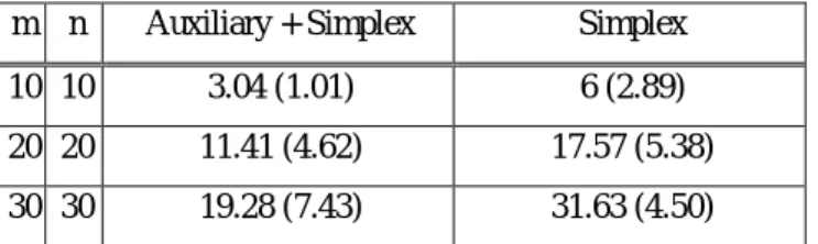
Table 2 shows the summary of the computational results. It shows that the auxiliary algorithm help the simplex method consistently reducing the number of required iterations by about 40%.

Table 2. The summary of the average numbers of total iterations required for the simplex

method. The numbers shown in the parenthesis is the associated standard deviation.

m n Auxiliary + Simplex Simplex

10 10 3.04 (1.01) 6 (2.89)

20 20 11.41 (4.62) 17.57 (5.38)

30 30 19.28 (7.43) 31.63 (4.50)

Here we propose an auxiliary algorithm for the simplex method. The auxiliary algorithm has the following advantages: there is no need to know the value of an optimal solution, and no special format for the problem is needed. It is a practical algorithm because its computation complexity is O(m+n). Furthermore, the

simplex method with this help can possess a better worst-case complexity bound than those without this help. Although there lacks a proof for the better global complexity for our method, we have explored its computational performance on some random test problems. The computational results show that the auxiliary algorithm

does help the simplex method consistently reducing the number of required iterations by about 40%. For future studies, we shall test it with more larger-scale problems as well as take the same test problems used in NETLIB for further comparisons.

4. Conclusion and Futur e Wor k

Here we propose an auxiliary algorithm for the simplex method. The auxiliary algorithm has the following advantages: there is no need to know the value of an optimal solution, and no special format for the problem is needed. It is a practical algorithm because its computation complexity is O(m+n). Furthermore, the simplex method with this help can possess a better worst-case complexity bound than those without this help. Although there lacks a proof for the better global complexity for our method, we have explored its computational performance on some random test problems. The computational results show that the auxiliary algorithm does help the simplex method consistently reducing the number of required iterations by about 40%. For future studies, we shall test it with more larger-scale problems as well as take the same test problems used in NETLIB for further comparisons.

5. Reference

[1] I. Adler, N. Karmarkar, M.G.C.

Resende and G. Veiga, An implementation of Karmarkar's algorithm for linear programming.

Mathematical Programming 1989; 44:

297-335.

[2] E.D. Anderson, and Yinyu Ye, Combining interior-point and pivoting algorithms for linear programming.

Management Science 1996; 42, (12):

1719-1731.

[3] K.M. Anstreicher, and P. Watteyne, A family of search directions for Karmarkar's algorithm. Operations Research 1993, 41, (4): 759-767.

[4] R.E. Bixby, J.W. Gregory, I.J. Lustig,

R.E. Marsten and D.F. Shanno, Very large-scale linear programming: A case study in combining interior point and simplex methods. Operations Research

1992, 40, (5): 885-897..

[5] S.C. Fang, and S. Puthenpura. Linear Optimization and Extensions,

Prentice-Hall, Englewood Cliffs New Jersey, USA, 1993.

[6] N. Karmarkar, A new polynomial-time

algorithm for linear programming.

Combinatorica 1984; 4: 373-395. [7] C.L. Monma, and A.J. Morton,

Computational experience with a dual affine variant of Karmarkar's method for linear programming. Operations Research Letters 1987; 6: 261-267. [8] M.J. Todd, A Dantzig-Wolfe-Like

Variant of Karmarkar's interior-point linear programming algorithm.

Operations Research 1990; 38, (6):