THE DESIGN AND ANALYSIS OF A SEMIDYNAMIC DETERMINISTIC ROUTING RULE

498 IEEE TRANSACTIONS ON COMMUNICATIONS, VOL. COM-29, NO. 4, APRIL 1981

The Design and Analysis of a Semidynamic Deterministic

Routing Rule

TAK-SHING P. YUM, MEMBER, IEEE

(Invited Paper)

A b s f r e T h e best deterministic rule, newly proposed in this paper is similar in nature to the best stochastic rule [3], except that 1) a maximum traffic bifurcation flow distribution is chosen and 2) deterministic routing sequences are used. Analysis shows that the best deterministic rule always gives better delay performance than the best r.tochastic rule. A semidynamic version of this rule is introduced for use in a varying traffic rate environment.

T

I. INTRODUCTION

HERE are four essential components of information that can be used by a routing rule in a computer-communica- tion network. 1) The topological information concerns the entire network. It includes, for example, whether a given out- going link can lead to a certain destination, number of hops from the originating node to each destination node, etc. It

is changed whenever the network is expanded, some parts of it are removed, or when nodes and links fail. 2) The traf- fic rate information accounts for the external traffic intensity

of each source and destination pair. It may change over a period of perhaps hours, in contrast to the topological in- formation which changes perhaps over days or even weeks. As an example in one region, the traffic may peak at certain hours during the morning and afternoon, and may decline considerably at night. 3) The local queue length information,

includes lengths of output queues, the types of messages in each queue, their priorities, etc., at each local node. 4) The

feedback information includes the state of the queues and other local information at neighboring nodes. Usually, only portions of this are fed back and used.

Rules which incorporate feedback information are called

feedback rules. Otherwise they are called local rules. Routing

rules that use the instantaneous queue length information for their routing decisions are called adaptive rules. Otherwise

they are called fixed rules. Adaptive rules have been shown to give better delay performance than the fixed rules, but their implementations are more complex. Fixed rules have been studied extensively in the literature [2]

.

Most of them are of the stochastic type, i.e., messages are distributed to the output buffers under a fixed probability assignment. One particular stochastic fixed rule that minimizes the average message delay is analyzed in [3]. We refer to it here as the BS (best stochastic) rule. We shall first summarize the BS

Paper received April 20, 1979; revised November 11, 1980. The author is with the Institute of Computer Engineering, National Chiao-Tung University, Hsinchu, Taiwan, Republic of China.

rule in the next section because it is the substructure of the BD (best deterministic) rule, the rule to be studied here.

In Section I11 we introduce the flow distribution entropy function H . We shall see that finding the flow distribution

of maximum H is essential for the efficient operation of the

BD rule. We then introduce the BD rule and discuss how it operates in a network under a varying traffic rate environment. In Section IV, we study the properties of the BD rule and compare its delay performance to the BS rule.

The primary purpose of this paper is to single out the routing aspect of the network operation and demonstrate,

through analysis, the improvement possible by using de- terministic routing sequences to bifurcate traffic. We would also like to emphasize that this kind of theoretical study pro- vides insight in “custom designing” routing rules for specific networks. It also points out the directions for improving net- work performance (more throughput, less delay) through the choice of routing rules.

Note that the BS rule is used primarily for network design purposes; there is no known implementation of it in any existing network. As for the BD rule, it is newly proposed. Deterministic routing sequences introduced here are being used in the Common Channel Interoffice Signaling (CCIS) network for telephone signaling. The use of the optimum flow distribution and the semidynamic version of the rule in the CCIS network is still under investigation.

11. THE BEST STOCHASTIC ROUTING RULE [3] , [ 101 The BS rule is globally optimum in the sense that it gives a minimum overall average time delay, averaged over all nodes of the network and averaged over statistically varying time delay due to traffic fluctuation, given that traffic is bifurcated (or routed to different outgoing links) by fuced probability assignments at each node. Here, we assume that the input

traffic rates are fixed. In situation where traffic rates do change, this rule can be operated in a semidynamic mode with new routing decisions calculated periodically from new estimates of the traffic rates. Algorithms incorporating this feature can be found in [ 4 ] , [5]. Let us consider a hypo- thetical computer communication network with N nodes

and L links. Let

Ci

be the capacity of link i in bits/s; Ai be the rate of average message flow over link i ; 1/11 the average length of exponentially distributed messages, assumed to be the same throughout the network; and yi, the external Poisson arrival rate of messages from node i to node j . After invoking the message length independence assumption [ 6 ] , 0090-6778/81/0400-0498$00.75 0 1981 IEEE

YUM: SEMIDYNAMIC DETERMINISTIC ROUTING RULE 499

the complex queueing network is reduced to a network of M/M/1 queues. The average time delay is

where Ti is the nonqueueing delay in link i (e.g., processing

delay, propagation delay, etc.), and

J;:

4

hi/^

is the flow in link i. Our routing problem is similar to the multicommodity flow problem in network-flow theory. The objective is’% assign paths for each commodity so as to minimize

T.

Let there be M source-destination pairs (or commodities) in the network and let the average flow in link i due to commodity k be denoted a s h k . Then

M

and the set C f i k } completely specifies the routing strategy. There are two constraints on ( f i k } . 1) The capacity constraints say that

J;:

<

Ci for all i. 2) the flow constraints say that mes- sage flows must be conserved, commodity by commodity. Thus, if we labei commodities by the source-destination nodal pairs, and links by the two nodes to which they are con- nected, we have at node I , due to comodity (i,

i)

(from [

l o ]

)

N N -yii/p if 1 = i

yiJp if I = j (3)

k= 1 m = l

0 otherwise.

There are various algorithms for solving this constrained minimization problem. The flow deviation (FD) method [3]

is the earliest one. The extrema1 flow (EF) method [7] and the gradient projection (GP) method [8] are more recent and execute in less time. They all use the iteration approach and rely on the fact that

‘T

is convex, as is the feasible set of multicommodity flows. Thus, a unique global minimum exists. The FD method provides the total flow

g.}.

.The

individual commodity flows ( f i k } required for routing assign- ment must be determined by additional “bookkeeping.”

III. THE BEST DETERMINISTIC ROUTING RULE The BD rule differs from the BS rule in two aspects: the choice of maximum traffic bifurcation and the use of de- terministic routing sequences. In this section, we shall first elaborate on these two and then discuss the operation of the BD rule in a network.

A . Maximum Traffic Bifircation

In the preceding section, we have indicated the use of the FD method, among others, to find the total flow

vi}.

Now for a specific set ofJ;:, say cf;:*}, there corresponds many sets of Cf;:k} satisfying (2). For the BS rule, it makes no dif- ference which set of

g.k}

is used, because they all result in the same delay. For the BD rule, however, we want t o find

the particular set C f k * } results in maxinlum triffic bifurca- tion, Now for an adaptive routing rule, more traffic bifurca- tion. means more traffic can be adaptively routed. And it

has been shown [I] that as the adaptive portion of traffic increases, relative to the fixed traffic, while keeping the total traffic constant, the delay performance improves. This is also true for the BD rule for the same reason.

To find C f i k * } ) , let us focus on a particular node, say node n . Let L , be the set of outgoing lirlks and define Pik

as the probability of routing the kth commodity to link i

at node n , or

Recall that our. objective is to find C f i k * } such that the traf- fic bifurcation in the network is maximum; This is equivalent to finding the set of Pik3 whose value are “as near to each

other” as pdssible at each node. Therefore, we can find

x.k*}

, by maximizing the traffic distribution entropy function’ H :

subject to the nonnegativity constraints f i k 2 0, the flow conservation constraints (3), and the link utilization con- straints (2).

It can be shown that H is a linear combination of convex

functions, and so is itself convex. The constraints are all linear. Therefore a unique maximum value of H exists and can Lie found by the same iterative technique prescribed in the last section. The flows

X}

and the initial guessed values of

g k }

are obtained from the solution of the optimization problem in the preceding section. The set {Pik*} which completely

specifies the routing strategy is calculated from

xk*}

at each

node via (4).

B. Deterministic Routing Sequences

each node, we can use a deterministic routing sequence

S,

k : Instead of assigning routes randomly according t o {Pik*} at

S , k = {SI, s 2 ,

...)

S m }

with si = 1 meaning a routink decision to send the ith incoming

messages of commodity k to outgoing iink 1 at node n. .

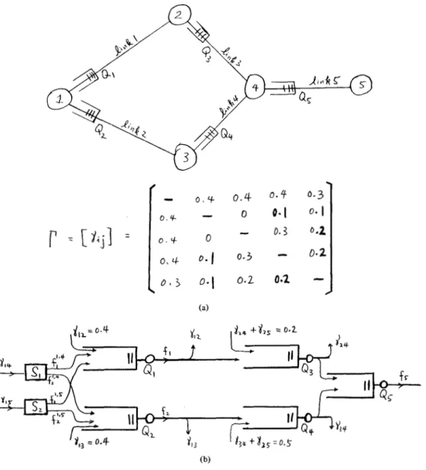
We now show how t o calculate the decision sequence via a simple example. Consider the queueing system of Fig. l(b), which is a model of the Singie node in Fig. l(aj. For the values of X1, A2, and

X

shown, P I and P2 are calculated to be 0.7 and

1 Any change toward equalization of the probabiiities {Pi”} increases H. MaximixingH therefore mdximizes the ambunt of traffic bifurcation.

500 IEEE TRANSACTIONS ON COMMUNICATIONS, VOL. COM-29, NO. 4, APRIL 1981

In a network, we first calculate Pik from f i k . We then de- termine the sequences S, from the Pik’s for each commodity

at each node. With the { S n k } determined, the routing rule is

completely specified.

As a final remark, we find out that the number of sequences we have generated are all recurrent. A closer study reveals the following theorem, which is needed in the analysis of the BD rule (Section IV). The proof is in the Appendix.

given by Pi = ni/N is recurrent with period N , where (nil and

N are relativeiy prime. C. An Example for Illustration

(a)

x,

=0.2 Theorem: The sequence of decisions S with rational Pi’s

Consider the five-node network in Fig. 2(a). Let

I’

= [ y i j ] be the input traffic matrix with yii the rate of external mes- sage arrival from node i to node j . All links are assumed to have a capacity of one and message lengths are also normalized X2

(b)

Fig. 1. (a) A network node with two outgoing links. (b) A twoqueue system, model of the network node in (a).

0.3. We want to find a sequence of decisions, say S =

11

2 1 1 2 e . . } such that the number of decisions of 1 (or on queue 1)

and the number of decisions on 2 have ratios as close to 7:3 as possible for any segments of S. Compare this sequence to the randomly generated sequence S’ where the probabilities of selecting “1” and “2” are 0.7 and 0.3, respectively. S ap- pears to be more “orderly.” Hence delay performance of the queueing system using S is improved when compared to that which uses $.,This we shall show in the next section.

For any subsequence of length r n , let D(l Ini) be the num- ber of 1-decisions and D(2 Im) = m - D(l Im) be the number of 2-decisions. We want D(i Im)/m, the fraction of messages to be routed to

Qi

in a total of

vi

message, lie as close to Pi as possible for all m. Therefore, starting from m = 1, we choose the decision (1 or 2 in this case) that minimizes

C;=

,.[D(;

Im)/m - P i ]

’

for each m . AS an example, S for the

X messages of Fig. l(b) is calculated to be S = {[I 2 1 1 1 2 1 1 2 11) where [.] means that the sequence inside is to be repeated In general, for the set of Pi’s, i = 1, 2,

-.,

Q , S is determined by the following algorithm.’

Step Q : - n = 1

to unity. For this simple network with symmetric input traffic and y i = 7 3 2 = 0, it is sufficient t o consider a unidirectional flow of traffic because the flow is the same in the reverse direction. If we focus on the flow from left to right, we have the queueing model and the rates of flow in and out of the queues as shown in Fig. 2(b). Using the BS rule for this simple

network, it is easy to see that all messages would follow their unique minimum hop routes except the y I 4 and the y 1 5 messages, which can be routed either through node 2 or node

3. How should these two message streams be bifurcated for

minimum average time delay is what we are going to investi- gate. The

fi

that minimizes (1) is given as cfl,

fz

, f3, f 4 , f5) = (0.8, 0.7, 0.6, 0.8, 0.8). Focusing on node 1 and its two outgoing links, we note that the four unknown flows due to individual commodities are f l ‘ p 4 , fz194, f l

’”,

and fZ1.’.

They are the flows due to y1,4 and yl, messages on links 1 and 2, respectively; and are related by the link utilization constraints (2) and the flow conservation constraints (3). Thus, from (2) we have

Noting that f l ‘ 2 ’ = y1 = 0.4 andfi 1 9 3 = 71 3 = 0.4, we

arrive at

f 1 1 r 4 + f 1 1 r 5 = 0.4

f21.4 + f 2 1 ’ 5 = 0.3.

And from (3), we have

= squared error in making an i-decision at

decision-node n . f 1 l S 4 + f 2 1 , 4 = y 1 4 ~ 0 . 4

Step 2: ek = min [min [ e l , e 2 , e 3 ,

-1 I

f l 1 9 5 + f 2 1 p 5 = y1 5 = 0.3. (9)

s, = k Here are four equations for four unknowns. But, unfor-

Step 3: n + n

+

1; GO TO Step 1. tunately, one of them is linearly dependent [ ( 6 ) added to (7) is the same as (8) added to (9)]. So the Cf;:k} cannot be 2 T~ demonstrate the efficiency of this algorithm, the above se- dniquely determined and We have a little freedom in choosing quence is calculated by hand. the values of the individual commodity flows. As explained

YUM: SEMIDYNAMIC DETERMINISTIC ROUTING RULE 501

(b)

Fig. 2. (a) The five-node network and the input traffic matrix. (b) The queueing model.

before, we want to choose the

u.k}

for maximum traffic bifurcation by maximizing H . For this example, we have

- - ~ = f , 1 - 4 10gf11.4 + f 2 l I 4

+flip5

10gf,'2~ + f 2 1 , 5 1 0 g f 2 1 3 5

--(J-~',~

+ f i 1 t 4 > -1og(fl1r4 + f 2 1 3 4 ) - ~ 1 1 9 5 + f 2 1 9 5 ) - l ~ g ( f ~ ' ~ ~ + f 2 1 , 5 ) = f l l p 4 logfl l r 4

+

2(0.4 -f1 1 , 4 ) log (0.4 -fl 1 , 4 )

+

(J-1 1 , 4 - 0.1) log l P 4 - 0.1)

+

2.390.

Differentiating H with respect to f1 setting the result equal to zero and simplifying, we arrive at f i 1 , 4 = 8/35. Hence f 2 1 9 4 = 6/35, f i ' x 5 = 12/70, and f i 1 p 5 = 9/70. The

7 1 4 traffic therefore is to be split into two streams with a

4:3 proportion for links 1 and 2 ; and for the y1 5 traffic, also a 4:3 proportion. This therefore is the maximum bifurcation

of traffic in node 1 while still preserving the flow rates on links 1 and 2 to be 0.8 and 0.7.

D.

Network Operation

In the operation of the BD rule in a network under a varying traffic rate environment, it is assumed that a network control center (NCC) exists and recalculates the optimum flow distribution (in the sense of the BS rule criterion) when- ever there are significant changes in the external flow pattern at the local nodes. It then determines the maximum traffic bifurcation of each commodity at each node by maximizing the H function. The patterns of traffic bifurcation (the Pik's)

are sent to the respective nodes. This can be done either periodically o r when necessary. Each node then generates the decision sequences from the Pik's received. The messages, after being classified by commodities (or their source-destination type), are then routed according to the decision sequences associated with their commodity.

502 IEEE TRANSACTIONS O N COMMUNICATIONS, VOL. COM-29, NO. 4, APRIL 1981 implementing the BD rule. It should be noted that we are not

documenting an existing rule. We are only pointing out the feasibility of this rule (or infeasibility, depending on the particular network being considered) based on some common technical requirements, such as traffic updates, computational overhead and traffic overhead.

1) Traffic rates usually vary during the hours of the day. Thus, they have to be updated periodically for efficient opera- tion of the network. Under unusual circumstances such as node and link failure, however, immediate update is required. As an example, the input traffic to the CCIS network is tele- phone call initiated. The rates generally do not vary very much in any 15 minute intervals. In 1141 , the ARF’A network HOST message arrival rate is shown on hourly basis. The update in- terval can be determined from these plots.

2) Computation of the optimum flow distribution is needed after each traffic update. There are two computational ad- vantages.

i) The flow distribution of the last update is a sub- optimal solution of the present update. Therefore, the time to reach the optimum solution is significantly less than the case where some arbitrary initial feasible solution is assumed.

ii) Due to random fluctuations, input traffic rates cannot be measured precisely. Therefore optimum flow distribution need not be highly a ~ c u r a t e . ~ As an example, in 131 it was reported that the optimum flow computation time for the 2 1

-

node ARF’A topology is 30 s (starting from an arbitrary initial feasible flow and with an accuracy of l o p 4 on T , the overall

average network delay). This is acceptable when the traffic update interval is in the order of minutes.

3) The local nodes need only send their estimates of the external arrival rates to the NCC when there is a significant change. On the other hand, a typical local node needs to re- ceive only the f i k values that is i) associated with its outgoing links and ii) changed significantly from their previous values. Thus if the traffic update is not too frequent, the traffic over- head in the use of the BD rule is minimum.

IV. THE ANALYSIS OF THE BEST DETERMINISTIC RULE

In this section, we first analyze the BD rule in an isolated network node and study two degenerate cases. We then gener- alize the analysis to arbitrary networks and show that the BD rule always gives lower delay than the BS rule.

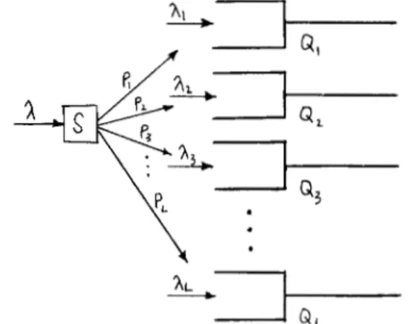
Consider an isolated network node with L outgoing links, all assumed to have the same capacity. Let Xi represent the rate of message arrivals that is constrained t o join queue i(Qi) and

X

represent the rate of message arrivals that is constrained to join Q, , Q 2 , ..., QL in proportion to P1 : P 2 : P3:

...

PL (Fig. 3). Using the BD rule, let us first consider the state description of Q,

.

Let N be the recurrence period of the rout- ing sequence and h(t); the position of the sequence at t. Then

h ( t ) = j with si = m means that the next arrival of the

X

mes- sage is to be routed to Q, . Denote 4 ( t ) as the number of

3 As an example, if the traffic rate is measured to t5 percent ac- curacy, there is n o need to compute the flow distribution any more accurately than, say, two significant figures (1 percent error).

-

Q3

L>

Fig. 3. An L-queue system with fiied arrivals to individual queues.

messages residing in Ql at t . The two quantities q 1 ( t ) and h(t) completely specified Ql at t . Hence [ q l ( t ) , h(t)] is an ap- propriate state vector for a Markov process. The number of states for h(t) is N and for 4 , ( t ) is M

+

1, where M is the

buffer capacity. The transition time between states has ex- ponential distribution. Hence we can solve the steady state behavior of Ql by representing it as a two-dimensional Markov chain. Define Si’(j) = 1 when s; = i - - otherwise. Thus if

s

={1 3 4 2 1 3 3 2 1

-1,

we have

s2

= ( 0 0 0 1 0 0 0 1 0

-1.

Let Pl(i, j ) = Prob[ql = i and h = j] . The state equations for Q, are

+ [ 1 - - S l ’ ( j - l ) ] - X . P l ( i , j - l )

+

X I P l ( i - l , j ) + P l ( i + l , j ) ] l < i < M - I \ d i m o d N

YUM: SEMIDYNAMIC DETERMINISTIC ROUTING RULE 503 The equations for other queues in Fig. 3 can be written

down and solved independently. The occupancy probability for Q , is

Pl(i) = Prob [i messages in Q1]

L

Fig. 4. A two-queue system with fixed arrivals suppressed. j = 1

1 The expected length of Q,, the overall delay, blocking prob-

abilities for different traffic streams, etc. can all be calculated in the usual way [ 101

.

To assess the delay performance of the BD rule, we con- sider two degenerate cases.

1) A two-queue system with arrival rate 2X (Fig. 4). Assum- ing 1/pC = 1, the utilization of each queue is p = X. The BS rule assigns incoming traffic to

Q 1

and Q2 with equal prob- ability. Using M/M/l result, the average delay of messages is

D s = l/($ -

X)

= 1/(1 - X). The BD rule routes arrival mes-

sages alternately to Q , and Q 2 ( S = { [ 1 21)). The interarrival time T of external arrivals is exponentially distributed with

mean 1/2h. Since every other message joins Q , , the interar- rival time of those messages joining Q , , denoted by T , is Tl = T

+

T . Its density has transform

2

F T I ( S ) =

[

"1

s +2X

This is the transform of the E, distribution. The BD rule therefore changed the Poisson statistic at the input end of the queue to the Erlangian statistic. By the technique in [9], the characteristic root of the above system is given by

(3 = FT1(l - a).

The unique root in ( 0 , 1) is u = (1

+

4h

-

4-/2. The average delay of messages in Q, is DD = 1/(1 - a). (By sym-

metry, the messages in Q2 have the same average delay.) To compare with the BS rule, we form the delay ratio

DD

_ -

_- 2(1 -X)

Ds 1 -'4X+4-

For p = X = 0.5, the ratio is 0.809. For p + 1, the ratio ap- proaches 0.75. The deterministic rule therefore gives 19-25

percent reduction of delay in the range 0.5

<

p

<

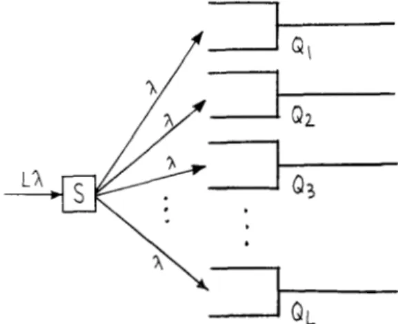
1 when compared to the stochastic rule.

2) An L-queue system with arrival rate LA (Fig. 5). The

BD rule degenerates to the sequential routing scheme with

S = { [l 2 3 ... L]}. By symmetry, the queueing behavior is the same for all L queues. The arrival rate for any particular

queue is LX/L = X. When L is large, the transform of inter- arrival time to Q , is

The interarrival time therefore, is a constant equal to 1/X

7

'

"

Fig. 5. An L-queue system with fixed traffic suppressed, S = {[ 1 , 2, ..., LI}.

and Q, is essentially a D I M I 1 queue (or equivalently an

E , IMI 1 queue). The characteristic root is given by u = 1

+

Xlnu. Comparing the delay with that given by the BS rule, we have

DD-

1 - u f l n u

Ds (1 --)In u

- -

For p = 0.5, u = 0.203, the delay ratio is 0.627. As p + 1,

u -+ 1, the delay ratio approaches 0.5. We conclude that when the fixed traffic is suppressed, and with L large, the reduction

of delay from the BS rule ranges from 37.3 percent to 50 percent in the range of 0.5 < p

<

1.

The analysis of the BD rule in a general network is similar to the join-biased-queue best stochastic (JBQ-BS) rule studied [ l ]

.

We first use the Poisson departure assumption? This assumption says that for local routing rules (Le., nonfeedback rules) with exponential messages, the departure process can be assumed as memoryless, or Poisson. It allows us to de- couple queues at different nodes and analyze them separately. We have shown how to analyze queues at local nodes. The overall average time delay and the overall average blocking probability can be calculated from Little's formula applied to a network [ l o ] .

We can actually prove that the BD rule always gives lower delay than the BS rule. The argument is quite simple: since the utilization of each link is the same for both rules, we only need to compare the average length of each queue. For each queue, the above analysis (the delay ratio DD/Ds) indicates that the BD rule (i.e., with Erlangian distributed interarrival time) always gives smaller average queue length than the BS 4 This assumption has been used in [ 121, [ 131, [ I ] and possibly many other similar works in the analysis of queueing networks.

5 04 IEEE TRANSACTIONS ON COMMUNICATIONS, VOL. COM-29, NO. 4, APRIL 1 9 8 1 rule (i.e., with exponential distributed interarrival time).

Since this is true for all queues (i.e., a network of Erlangian queues compared to a network of MIMI1 queues), we con-

clude that the BD rule always gives lower delay than the BS

rule. Further, this argument is independent of the network size, the network topology and the input traffic assumed.

We refer the reader to [l I ] for an example of the applica- tion of the BD rule to the Common Channel Interoffice Signaling (CCIS) network for the telephone system.

V. SUMMARY AND CONCLUSION

We started our discussion with a brief view of the BS rule and continued on to make an extensive study of the BD rule. The BD rule was shown to always give lower delay than the BS rule and has the best delay performance among the fixed rules5 in the literature. The operation of the BD rule in a varying traffic rate environment was described and its feasi- bility based on some common technical requirements was discussed.

APPENDIX

PROOF OF THE THEOREM IN SECTION 111 Let us decompose the sequence generated into a sum of L

subsequences: S = S1

+

S2

+

...

S L where L is the number of

queues in the system. Si has the property that all non-i- decisions are set to zero. Thus if

S = { 1 3 4 2 1 3 3 2 1 . . . }

we have

Sz = ( 0 0 0 2 0 0 0 2 0 - 9 ) .

Si contains all the information needed for Qi for routing. Consider the kth decision of S 1 , where m*N

<

k

<

( m

+

m is any nonnegative integer. Suppose for the ( k - 1) past decisions,

I

decisions are on 1 and k - 1 - 1 decisions

are on 0, or others. The decision rule for the kth decision will then be

mnl

+

(z+ 1 ) n l n l mnl

+

1 m N + k

- _

2 - - _ _ _ _

N o N m N + k by the given algorithm. Simplifying, we have

1

N[2mn1

+

22

+

11 S 2 n l [ m N

+

k ] ( A l l 0

Now consider the ( k

+

N)th decision; the decision rule is given as

2(m

+

l)n,

+

2k

+

1 2n, ( m + l ) N + k 0 N

2

-.

5 These are the rules which d o n o t use the instantaneous queue length information in making routing decisions.

Upon simplifying, we have

1

N [ 2 m n I

+

21

+

1 1 2 2 n , [ m

+-

k]. ~

0

Comparing with (Al), we observe that the kth decision is the same as the ( k

+

N)th decision. Since the above is true for arbitrary m , k , N , and n l , we conclude that the sequence S1 is recurrent with period N . We can go through the same argu- ment for Q 2 , Q 3 , *-, etc., and establish that all Si’s are recur-

rent with period N . Now since S is the sum of all the Si’s, it is easy to see that S is also recurrent with the same period.

The case where equality holds in ( A l ) needs further ex-

planation. This is the case where routing the incoming mes- sage to Q, or some other queues results in the same “error.” Step 2 of the algorithm uniquely determined the queue to be selected. Since this determination depends only on the numbering of queues, the ( k

+

N)th decision will be the same as the kth decision. Therefore, we conclude that blocks

of N decisions located anywhere in S is recurrent.

REFERENCES

T . Yum. “Analysis of adaptive routing rule in computer com- munication networks,” Ph.D. dissertation, Columbia.Univ.. 1978. J . McQuillan. “Adaptive routing algorithms for distributed com- puter networks,” BBN, Inc. Rep., May 1974.

L. Fratta, M. Gerla. and L. Kleinrock. “The flow deviation method.” Networks. vol. 3, no. 3 . 1973.

T. Stern, “A class of decentralized routing algorithms using

relaxation,” l E E E Trans. Commun.. vol. COM-25, Oct. 1977. R. G . Gallager, “A minimum delay routing algorithm using

distributed computation,” IEEE Trans. Commun., vol. COM-25. Jan. 1977.

L. Kleinrock, Communication Nets. New York: McGraw-Hill, 1964.

D . G . Cantor and M. Gerla, “Optimal routing in a packet-switched computer network,” IEEE Trans. Cornput.. vol. C-23. Oct. 1974.

M . Schwartz and C. K. Cheung, “The gradient projection al-

gorithm for multiple routing in message switched networks,” IEEE Trans. Commun., vol. COM-24. Apr. 1976.

Wiley, 1975.

I.. Kleinrock, Queueing Systems, Vol. I : Theory. New York: M. Schwartz, Computer-Communication Network. Design and Analvsis. Englewood Cliffs. NJ: Prentice-Hall, 1977.

T. Yum, “A semidynamic deterministic routing rule in computer communication networks,” in Proc. Nat. Telecommun. Conf., Washington, DC, Nov. 1979.

G . L. Fultz, “Adaptive routing techniques for message switching computer-communication networks.” Univ. California, Los

Angeles, Eng. Rep. UCLA-ENG-7252, July 1972.

A. Livne, “Dynamic routing in computer-communication net- works,” Ph.D. dissertation, Dep. Elec. Eng., Polytechnic Inst. New York, 1977.

L. Kleinrock, Queueing Systems, V o l . 2. Computer Application. New York: Wiley-Interscience, 1976. ch. 6. Fig. 6-26.

*

, ,

’ , Tak-Shing P. Yum (S’76-”78) received the

”:.

B . S . . M . S . . Ph.D. degrees from Columbia

’ j , University, New York, NY, in 1974. 1975. and

‘,’,e 1978, respectively.

From 1978 to 1980, he was a member of the

I Technical Staff at Bell Laboratories. Holmdel.

i.T, ..,.,’<‘pI *,’ <e*’~;&*-*

* ^ I -*-& < NJ, and worked in the area of data communi-

cations. mainly on dynamic routing, flow con- trol. traffic engineering, and performance analy- sis of the Common Channel Interoffice Signaling Network. In September 1980, he joined the National Chiao-Tung University of Taiwan. where he is now Associate Professor in the Institute of Computer Engineering. His main research interest is in the design and analysis of computer-communication networks and in the performance analysis of computer systems.