ADAPTIVE BLIND EQUALIZATION USING 2ND-ORDER AND HIGHER-ORDER STATISTICS

132 IEEE JOURNAL ON SELECTED AREAS IN COMMUNICATIONS, VOL. 13, NO. I , JANUARY 1995

Adaptive Blind Equalization Using

Second- and Higher Order Statistics

Fang

B.

Ueng and Yu

T.

Su

Abstruct- This paper presents two classes of adaptive blind algorithms based on second- and higher order statistics. The first class contains fast recursive algorithms whose cost functions involve second and third- or fourth-order cumulants. These algorithms are stochastic gradient-based but have structures similar to the fast transversal filters (FTF) algorithms. The second class is composed of two stages: the first stage uses a gradient adaptive lattice (GAL) while the second stage employs a higher order-cumulant (HOC) based least mean squares (LMS) filter. The computational loads for these algorithms are all linearly proportional to the number of taps used. Furthermore, the second class, as various numerical examples indicate, yields very fast convergence rates and low steady state mean square errors (MSE) and intersymbol interference (ISI). MSE convergence analyses for the proposed algorithms are also provided and compared with simulation results.

I. INTRODUCTION

HE PURPOSE of blind equalization is to recover the

T

intersymbol interference and noise corrupted signal from the received signal without the help of a training signal. Earlier investigators like Sat0 [l], Godard 131, and Benvensite and Goursat [ 2 ] used different LMS-type algorithms to deal

with this problem. Since the second order cumulant (i.e., autocorrelation function) is completely blind to the phase property of the channel to be identified, if the channel is not minimum phase, these algorithms may not be capable of generating correct results. Statistics of higher order must therefore be considered in the realization of blind equalization of nonminimum phase (NMP) channels.

Giannakis [5] has showed that the impulse response of an FIR filter can be determined from the cumulants (third- or fourth-order) of the filter output alone, In other words, cumulants can be used to estimate the parameters of a MA model without any a priori knowledge of the transmitted data, if the input distribution is not Gaussian. His result was further extended to identify linear, time-invariant NMP systems with non-Gaussian correlated input sequences [4]. Swami and Mendel [ 6 ] derived a recursive algorithm for estimating the coefficients of an MA model of known or- der using autocorrelations and third-order cumulants. Zheng and McLaughlin [9] proposed an algorithm that uses closed- Manuscript received September 15, 1993; revised June 17, 1994. This work was supported in part by the National Science Council of Taiwan under Grant NSC 82-0404-D-009-024. This work was presented in part at the 1993 Wireless Communication Workshop, Chung Cheng University, Chia-Yi, Taiwan, September 17, 1993.

The authors are with the Department of Communications Engineering,

National Chiao Tung University, Hsinchu 30035, Taiwan.

IEEE Log Number 9406083.

form formula to obtain an initial estimation and proceed to adaptively minimize the squared estimation error of the third order cumulants. Tugnait [7] used the total squared matching errors of various second and fourth-order statistics as the cost function to identify an ARMA model. Hatzinakos and Nikias

[8] presented an adaptive blind equalization method using the

complex cepstrum of the fourth-order cumulants (tricepstrum). Alshebeili, Venetsanopoulos, and Enis Cetin [ 101 suggested the use of second-order and all samples of third-order cumulants or the diagonal slice of bispectrum to identify FIR systems. Porat and Friedlander [ 111 described a nonlinear algorithm using the second- and fourth-order moments of the symbol sequence for equalizing QAM signals. All these algorithms are based on some closed-form relations between the parameters to be identified and the observed signal’s cumulants of various orders or their Fourier transforms called polyceptra. For the application to channel equalization, extra steps are needed to use the estimated system parameters to recover the transmitted signal.

Shalvi and Weinstein (SW) [I21 avoided these extra steps by devising new cost functions based on a necessary and sufficient condition for achieving zero IS1 in nonminimum phase linear time-invariant channels. Recently, they developed [ 131 another two blind deconvolution algorithms that render learning speeds much faster than those of their earlier proposals in [ 121. Since SW algorithms were aimed at removing ISI, the resulting MSE

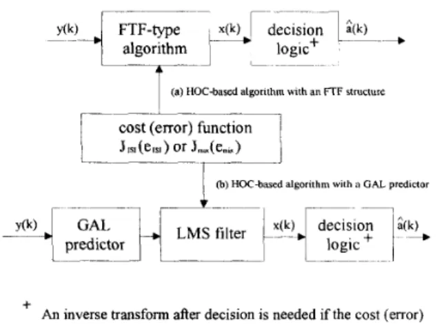
are often not as small as desired. Moreover, the convergence rate improvement of the second class of SW algorithms [13] was obtained at the expense of higher complexity and less flexibility for real-time implementation. Thic paper presents two classes of blind equalizers (see Fig. 11 that possess the properties of 1) fast learning speed, 2 ) small steady-state IS1

and MSE, and 3) low computing complexity. A system model

is introduced and candidate cost functions for achieving zero IS1 are discussed in the next section. In Section 111, we propose cost (error) functions for minimizing both IS1 and MSE and

present a fast transversal filter structure to perform multidi- mensional minimization of these cost functions. Another class of algorithms (Section IV) divide the equalization process into two stages. The received samples are whitened by a GAL filter in the first stage. The output sequence is then fed into a regular LMS filter (the second stage). In Section V, we provide computer simulation results on the IS1 and MSE performance of various proposed algorithms and make comparison with the theoretical MSE behavior, which is analyzed in Appendix A. A brief summary and some conclusions are given in

Section VI.

UENG AND SU: ADAPTIVE BLIND EQUALIZATION I33 lC?(O; 0)l = E[3:”k)]Cs”(l) 1 1 ~- ~ ( k )

4

FTF-type x ( k )

1

decision

-

algorithm

Id

10g,c+

5 1E[.3(k.)]lCl,S(l)l2

1 -_-I L

(a) HOC-based algorithm with an FTF structure

t

--

cost (error) function

JrSl(esl) or Jmu(emu)

+ An inverse transform after decision is needed if the cost (error) function used depends on third-order cumulants

where 8 stands for convolution, must be of the form

s = ,.io((). . . I . . .0). ( 5 )

When such a condition is satisfied, the distribution (or all cumulants) of the equalizer output is equal to that of the channel input data. In other words, the responsibility of a zero-forcing equalizer is to adjust its tap weights such that the instantaneous distribution of its output converges to the desired distribution [ 141. Shalvi and Weinstein [ 121 simplified this requirement to one that involves only second- and fourth-order cumulants. They consider the combined channeUequalizer system { s ( , i ) } and showed

E [ 2 ( k : ) ] = E[a2 ( k ) ]

Cl

s( 1 )

l2

(6)

1

Fig. 1. Classification of the proposed blind equalizers; .JISI ( q s i ) = cost (error) functions for minimizing 1st; . J L ~ S E ( P ~ , ~ + : ) = cost (error) functions for minimizing MSE, .Jr,,iX = f ~ ( . J r - ; i . Jw.E). p,,,, = f r ( ( . i s i , wsr.).

and

(7) 1

11. PROBLEM FORMULATION AND HOC-BASED CRITERIA

Let an i.i.d. sequence of symbols { ~ ( k ) } be transmitted through a linear time-invariant channel, then the equivalent baseband output sequence {y(k)} can be written as

y(k) = C b ( y ) a ( k : - / )

+

u ( k ) (1)

where the additive noise { n( k ) } is a white Gaussian sequence

and {b(i)} is the channel impulse response. Suppose the

channel output sequence y(k) is fed through an FIR-type equalizer with impulse response h ( i ) , i = 0, 1 , .

.

.

.

M then the filtered sequence becomes

!If

r ( k ) = C h ( i ) g ( k - 6 ) . ( 2 )

1 = 0

The purpose of a zero-forcing (i.e., intersymbol-interference elimination) equalizer is to find h = [h(O), h ( l ) , . . . , h ( M -

l)] such that the combining of the channel and the equalizer has the effect of a distortionless filter. In other words, the 2-transform of the perfect zero-forcing equalizer is equal to l / B ( z ) , B ( z ) being the 2-transform of the channel impulse response { b ( i ) } . Denoting the 2-transform of h by H ( z ) . we can describe this condition as

(3) where L B ( z ) is the phase of B ( z ) . The magnitude of H ( z ) can be estimated by using second-order statistics alone but not its phase. Hence, a suitable criterion should be a function of both second-order statistics and HOC’S.

On the other hand, zero IS1 requires that the taps { h ( z ) } be such that the output z ( k ) is identical to the input a ( k ) up to a constant delay. That is, the combined channel-equalizer impulse response

s ( i ) = hoi) 8 b ( i ) = Ch(i - I ) b ( l ) (4) 1

where E [ - ] denotes the expectation operator and the fourth- order cumulant C ~ [ Z ] is defined by

(8) C4[2] = E[27 - 3E[z”].

I34 IEEE JOURNAL ON SELECTED AREAS I N COMMUNICATIONS, VOL. 13, NO. I, JANUARY 1995

1 r - - - -_ -_ ~

Note that the inequality (9) also implies that the object function

is minimized by (5). These facts immediately suggest that

blind zero-forcing equalization can be accomplished by ap- plying a stochastic gradient-based method to perform either the constrained maximization ( 1 2), (1 3 ) or the unconstrained

minimization of (15). Another approach suggeted by Shalvi and Weinstein [ 131 was motivated by the observation that the transformation

~ ’ ( 7 1 ) = S ” ( T L ) [ S * ( ~ L ) ] ~

where s ( n ) is the vector representing the combined chan-

nel/equalizer impulse response at the nth iteration and p

+

q 2

2, followed by the normalization

s ( n

+

1) = S ’ ( 7 L ) / ~ ~ S ’ ( , / L ) ~ ~

causes the combined impulse response { s ( k ) } to converge

quickly to the desired response (5). Two algorithms based on this fact, one in batch mode the other in sequential mode, were proposed in [ 131.

All these algorithms, as mentioned before, were designed to eliminate ISI. Their MSE performance is often not satisfactory

and in some cases is unacceptable (see Fig. 2). Moreover, a stochastic gradient algorithm using (IO), (13), (14), or (15)

as its cost function is sensitive to the characteristic of the transmitting channel (see Fig. 5). The fast algorithms of [13] are more robust but require a complexity of O ( M 2 ) where

11.1 is the equalizer length; they are not particularly suitable

for real-time operation either. Moreover, the batch-processed super exponential algorithm of [ 131 may exhibit undesired jittering after it converges [see Fig. 7(a)]. Algorithms proposed

below will not have these shortcomings.

111. HOC-BASED ALGORITHMS WITH AN FTF STRUCTURE Although the functions defined by (14) and ( 1 5) are suitable criteria for minimizing ISI, minimum MSE cannot be achieved by using either of them alone. In fact, it can be shown that in an additive white Gaussian noise channel the minimum MSE solution leads to

where B ( w ) is the discrete Fourier transform of { h ( i ) } and No is the one-sided power spectral density of the additive

channel. In the presence of noise the zero IS1 upper bound max { C 4 [ x ( k ) ] } = C 4 [ a ( k ) ] cannot be attained either. As the noise level No increases, the constraint of searching on the surface of the unit ball { s :

cl

1 . ~ ( 1 ) 1 ~ = I} (i.e., E [ x 2 ( k ) ] =

E [ a 2 ( k ) ] ) will drive the tap-weight vector h(k) further and further away from the minimum MSE solution which must be obtained from the surface { s :

cl

1 . ~ ( 1 ) 1 ~ = u2}. An apprpriate solution is to add to the HOC-based cost (or error) function a term which reflects the magnitude of the MSE under blind circumstances. MSE involves only second-order statistics and cost (error) functions for minimizing the MSE of a blind equalizer have been presented before [ 11-[3]. The following error function is a good candidate for minimizing both IS1 and MSE:

where k;’s are appropriate weighting factors, & ( k ) =

hard-decision output based on ~ ( k ) , e d d ( k ) = G ( k ) - x ( k )

is the decision-directed error signal, e R a ( k ) = z ( k ) -

CY sgn [ x ( k ) ] ! and CY = E [ u 2 ( k ) ] / E [ I [ ~ , ( k ) I ] . Note that the inclusion of e d d ( k ) and ledd(k)l in ea. hoc serves two related purposes: 1) to measure the quality of the current equalizer output or the “distance” from the current estimation of { s ( i ) } to the desired response and 2) to offer an automatic switch between the start-up period and the standard transmission mode [2].

Another possible error signal can be obtained by considering the error signal used in the super exponential method [13] which updates the equalizer’s tap-weight vector by

h(k) = h(k - 1)

+

- Q ( k ) [ x 2 ( k )

B

- ~ , v L : ] : c ( ~ )

6

- S z ( k ) y ( k ) (18) where rn; = E [ a 2 ( k ) ] ,

io

is a constant, y ( k ) = [y(k), y(k -

l), . . .

,

y ( k - M

+

1)IT, S = C ~ [ c ~ ( k ) ] / E [ l a ( k ) 1 ~ ] and Q ( k )

is an estimator of the matrix RL1/m;, RL = E [ y ( k ) y ’ ( k ) ] .

In [13], Q ( k ) is updated by another recursive formula which must be initialized by batch processing a large data segment

first. We now present an algorithm that a) does not need initial batch processing, b) has a very small MSE, c) is insensitive to the eigenspread of the received data, and d) requires an O ( M )

UENG AND SU: ADAPTIVE BLIND EQUALIZATION 135 TABLE I

THE SW2-FTF BLIND EQUALIZER

e j (n1n - 1) = F' ( n - l ) y ( n ) = apriori forward prediction error (a)

(b)

(C)

(4

0 ( e )

? f ( n I n ) = y f ( n ) e f ( 7 f l n - 1) = apostenon forward prediction error

E f ( n ) = E f ( n - 1 )

+

r f ( u l n ) ~ f ( 7 t l 7 7 - 1) = accumulated forward prediction error

r(n) = Sf(R)Ef(" - l)/EJ(?Z) k,q,f(nln

-

1) =

F ( n ) = F ( n - 1 ) - rf("I71 - 1)

"

1

= forward prediction filter

complexity only. b) and c) can be accomplished by replacing (18) with

a) and d) are achieved by first defining the time domain autocorrelation matrix

k

(20)

.J+!

and replacing in (16) by R - l ( k ) . Noting that the un-

weighted correlation matrix k R ( k ) and its inverse can be

computed recursively in a way similar to that in a recursive least-squares method [ 181, we define the forward predictor's Kalman gain vector as

It follows [IS]

R - l ( k ) y ( k ) = - y ( k ) k M ( k l k - 1) (22) where y( k ) is the so-called conversion factor. Substituting the above equation into (19), using the analogy between the resulting equation and the recursive relation governing the update of the tap-weight vector for the FTF algorithm, and after some algebraic manipulations we obtain the blind equalizer described by Table I. This algorithm will be called the SW2-FTF algorithm henceforth. The same approach can be applied to other cost (error) functions [(lo), (13)-(15), or (17)] with proper modifications made on steps ( m ) and (71) of

Table I. The resulting algorithms all have the same order of complexity and enjoy the same advantages [i.e., (a)-(d)].

When the constrained minimization of 53 is implemented the transmitted data sequence has to be transformed first unless it has a nonzero skewness (i.e., E [ a 3 ( k ) ]

#

0. If the i.i.d. sequence { a ( k ) } is generated from a (normalized) PAM signal

set

{Si}

defined by

with p(Si) = 1/2M. then the nonzero cumulant requirement cannot be met. To solve this problem, [9] used the nonlinear transform:

Si = In [ K ( 2 M

+

S i ) ] - po (24)

where K E [ 1 / 2 M , 3/4M] is a compression factor and

po = E { [In [ K ( 2 M

+

S ; ) ] } . At the receiving end, to restore the original transmitted signal, it is necessary to make the inverse transformation

at the decision output (see Fig. I). Instead of (24), (25) we suggest that the following simpler transform pair be used to accomplish the same purpose

where

2123-1

p , - ( S i + 2 M ) 2 a = - ( 2 A - 1 )

136 IEEE JOURNAL ON SELECTED AREAS IN COMMUNICATIONS, VOL. 13, NO. I , JANUARY 1995

TABLE I1

THE L-HOC BLIND EQUALIZER

B The transversal filter

h , ( k + I ) = h , ( k ) - ~ " ~ , h ~ ~ ( k ) e ~ ( l i - - ) h , ( k ) IS the zth tap weight at the kth iteration

The transversal filter input I S the last stage output of the lattice filter

IV. HOC-BASED ALGORITHMS USING A GAL PREDICTOR

Although the above HOC-based blind algorithms have low computational load, their convergence time can still be re- duced. It has been shown [ 151 that the start-up period can be shortened if the channel correlation matrix is orthogonalized. This can be attained by employing a whitening filter in front of the equalizer. We already know that [ 14, ch. 141 if the input of a lattice filter is wide-sense Markov of order M , then the forward prediction error produced at the Nth stage lattice filter, N 2 M , is white. Taking the Nth prediction error as the input to an HOC-based adaptive algorithm (like those mentioned in the previous section), we then obtain an equalizer that puts the responsibilities of estimating l/JB(z)l and L B ( z ) separately

on two cascaded processes. Such a division of labor should be

able to increase the learning speed. We now describe a new class of algorithms. All of them use a lattice predictor as a preliminary equalizer.

Let us consider the processing of the predictor output and ignore at first the GAL filtering part. Recall that the muItidimensiona1 Newton search results in the recursion [ 15, ch. 41

(28)

a 7

h(,n

+

1) = h(71) - p R i l -

ah

where 7 is the designed cost function and RL is the au- tocorrelation matrix. The major difficulty in implementing this algorithm is the computing of the autocorrelation matrix RL. The computing complexity can be greatly reduced if the sequence {y(n)} is white which, as just mentioned, can be obtained by letting {y(n)} pass through a lattice filter and taking the pth ( p

2

q, q being the length of the channel's impulse response) stage forward prediction error {e: ( n ) }

as the output. Redefining the input vector of the Newton algorithm as y(n) = [e,'(n)eg(n - 1 ) . .

.

e z ( n -

A4

+

l)]'

we can express the autocorrelation matrix as RL = diag (E[e:2(n)], E[e;2(n - l ) ] . . .

.

,

E [ C ; ~ ( ~ - M

+

l ) ] ) . (29) The ensemble averages, ~!3[e,'~(l)], 1 = 71. n-1,. .

. ,

n-kf+l.

can be estimated by time averages

For n sufficiently large all these estimators will approach a

constant A and therefore RL = A I , I is the identity matrix. Now the recursion (28) can be written as

where p' = PA. Replacing

-,d(dl/ahi)

in the above equation by the product of y ( n ) and the error function e2, hoc

defined by (17), we then obtain the algorithm presented in Table 11. This algorithm will be referred to as the lattice- & h o c or the L-HOC algorithm. Again, the same approach can be employed to generate algorithms with different cost (error) functions for the second stage filter. We will omit the extensions to these cases and use L-HOC as a representative of its class.

As a remark, it is well-known that if {b(i)} is mini- mum phase then the prediction error (innovation) y(k) -

E[y(k)ly(k - l), y ( k - a ) , . - . ] is equal to c a ( k ) where c is a constant. So if the transmitting channel is minimum phase, an equalizer with a GAL predictor (or any other whitening prefilter) should converge faster than one without (see Fig. 6).

v.

SIMULATION AND NUMERICAL RESULTS To demonstrate the usefulness of the proposed algorithms, computer simulations for equalizing the following channels are performed.

Channel I (eigenspread = 10.5, zeros at 7.1, -0.24 f

Channel 2 (eigenspread = 41.5, zeros at -2.1. -0.48): Channel 3 (eigenspread = 95.9, zeros at -1.8, -0.55): Channel 4 (eigenspread = 150, zeros at -1.67, -0.6): Channel 5 (all-pass channel):

0.19i): B1 = [-0.15 1 0.5 0.11. Bz = [0.3887 1 0.38871. B3 = [0.42 1 0.421. B4 = [0.44 1 0.441. i

<

0

r.

0.84* 0.1"', t

>

0 h, = -0.4, t = 0 .

We use both the MSE and IS1 measures in assessing the proposed algorithms' performance. IS1 is defined as

UENG AND SU: ADAPTIVE BLIND EQUALIZATION 137

1

10,

"0 SIN1 IIIINI 1500 ZIx)0 251x1 30011 35011 number of iferations

(b)

Fig. 3.

algorithm, ( 2 ) B-G algorithm, (3) Sato algorithm, (4) J4-FTF algorithm.

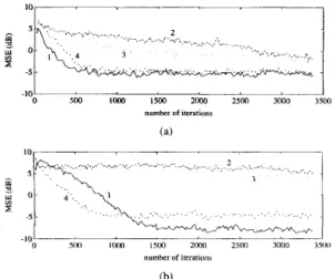
MSE learning curves for (a) Channel I (b) Channel 2; (1) L-Jd

where lslrnax is the maximum absolute value of the impulse response of the combined channeUequalizer system { s ( I ) } . All numerical results were obtained with a hundred runs. For HOC-based lattice or transversal filter we choose / I = 0.00001

and p. = 0.0002 is used for conventional blind algorithms. All filters hav a length of 15 taps. Besides the SW2-FTF and the L-HOC algorithms, we also compare the Sat0 algorithm [ 11, the Beniste-Goursat (B-G) algorithm [2], the J4-LMS algorithm (one that uses the cost function 54 with LMS filtering), and the L-.J, algorithm (GAL predictor followed by J4-LMS). The performance of the SW algorithms of [I21 is not included since they and the .J4-LMS algorithm have similar learning behavior.

Fig. 2 exhibits IS1 behaviors for the Jd-LMS, the J4-FTF

algorithms and two conventional blind equalizers at SNR = 30

dB. Obviously, the algorithms using J4 as the cost function have a learning speed faster than conventional blind equalizers. Convergence speed improvement brought about by the FTF- based algorithm in identifying NMP channels can be found in Fig. 2 as well. In Fig. 3 the MSE performances of 1) the

L-J4 algorithm, 2 ) the B-G algorithm, 3 ) the Sat0 algorithm,

and 4) the JA-FTF algorithm are compared. It can be seen that the two HOC-based algorithms far outperform the other two. At SNR = 3 0 dB, convergence (MSE

5

- 5 dB) can be expected within 1500 iterations. Unfortunately, the steady- state MSE's of both HOC-based algorithms are relatively high. This drawback is removed by the addition to the original error signal of a term which measures the MSE, as can be seen from Fig, 4 where improvements of 80 (Channel 1) and 25 dB (Channel 2) are obtained. On the other hand, it indicates that the improvement is a decreasing function of the eigenspread The influence of the channel eigenspread is also shown in Fig. 5 : when the eigenspread is large, the learning speed of

the JA-LMS algorithm (or those proposed in [ 121) becomes so slow that the algorithm is of no practical use any more. Fig.

6 compares the learning curves obtained from both simulation and analysis. These curves confirm the correctness of our

of RI,.

2

. . .~

(b)

Fig. 4.

(2) L-.J4 algorithms; (a) Channel I . (b) Channel 2.

Thermal noise free MSE performance comparison of ( I ) L-HOC and

MSE analysis; they also indicate that the recursive formulae derived in the Appendix are useful in predicting the MSE learning behavior. The effect of GAL filtering can be found from Fig. 6(b): curve 3 represents MSE performance of the

L-,J4 algorithm when equalizing a channel that resulted from

cascading a minimum phase channel with Channel 5-an all- pass channel, and curve 4 is corresponding MSE performance of the Jd-LMS algorithm. Finally, in Fig. 7, we show IS1 and

MSE learning curves for SNR = 10, 20, 30 dB, respectively.

We find out that both the steady-state IS1 and MSE are

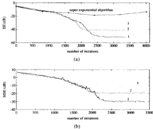
sensitive to thermal noise. The effectiveness of ~ ( k ) is clear: a 30 dB and 25 dB degradation on IS1 and MSE performance results when the SW2-FTF algorithm is replaced by either the superexponential algorithm [Fig. 7(a)] or the J4-FTF algorithm [see Fig. 3(b) and Fig. 7(b)]. Also shown in Fig. 7 is the IS1 behavior (circled points) of the batch-

processed super exponential algorithm [ 131. We notice that its IS1 does not remain stable after the algorithm converges.

This is because this approach uses estimations of equalizer output HOCs to evaluate desired tap-weights { h( I ) } and the

IS1 measure is sensitive to estmation errors when the equalizer is at equilibrium. Such a jittering phenomenon can be avoided if we increase the batch size; but then the fast convergence advantage of this algorithm will no longer exist.

VI. CONCLUSIONS

This paper presents two classes of adaptive blind algorithms based on second- and higher order statistics. The first class consists of FTF based algorithms whose cost functions involve second and third- or fourth-order cumulants. The second class uses a gradient adaptive lattice predictor cascaded with an HOC-based stochastic gradient algorithm. The FTF-type algorithm used by the first class necessitates a numerical stabilization scheme [20] when implemented in finite-precision environment. The second class, on the other hand, is numer- ically stable, for both its first stage (GAL) and second-stage filters are. The computational loads for these algorithms are all linearly proportional to the filter length: the first class

I38 IEEE JOURNAL ON SELECTED AREAS IN COMMUNICATIONS, VOL. 13, NO. 1, JANUARY I995

number of iteratrons (b) Fig. 5.

mance; (a) Channel 3; (b) Channel 4.

The effect of channel characteristics on the equalizer's MSE perfor-

- 1 0 " " " ' ~ ' I

0 100 2 M 31K) 400 SO0 6Oil 700 XI10 900 1lXl0

number of iterations

(b)

Fig. 6. . J - L M S algorithm's MSE learning curves estimated by simulation ( I ) and analysis (2); (a) Channel 2, (b) Channel 5. (3) and (4) are the MSE learning curves for the L J 4 and .J4-LMS algorithms, when equal-

izing the channel which is the combination of the minimum phase channel

Bs = [0.80.30.1] and Channel 5.

requires a complexity of O ( 9 M ) when its stabilized version

is used; the second class needs O(GM) only. As various numerical examples have shown, these new algorithms give very fast convergence rates, robustness against eigenspread variations, low steady-state MSE and ISI, and are suitable for real-time implementation. Simulation results also show that their learning behaviors are consistent with what the analysis had predicted.

APPENDIX A CONVERGENCE ANALYSIS

A. General Results

This Appendix provides MSE analysis of the proposed algorithms, assuming known signal constellation and channel impulse response. We follow the approach suggested in [ 191

----.----.

-30L--

-.-_-

--

' A

0 5011 I O 0 0 I S M 2IWM ? 5 M X K Y I 3Xx) -40 number of aera1,ons (b)

Fig. 7. The influence of the noiw power level on the (a) IS1 and (b)

MSE performance of the J2,h0,-€TF algorithm in equalizing Channel 2;

(1) S N R = 30 dB, (2) SNR = 20 dB, ( 3 ) SNR = 10 dB. The learning curve

of the batch-processed super exponential method at SNR = 30 dB 1s also

shown (circled points).

where a recursive method is used to evaluate the time- evolution of the MSE. The basic assumptions used are':

1) The data symbols, a ( k ) are zero-mean independent and identically distributed symbols derived from a PAM data constellation.

2) The tap-weight vector h(k) is independent of the equal-

izer input vector y ( k ) .

3) The equalizer output ~ ( k ) , conditioned on a ( k ) and

h ( k ) , is zero-mean with variance c?(n).

In general, the recursive formula governing an equalizer's

(A. 1) where C ( k ) is an

A4

x M matrix and e ( k ) is the error signal

at the kth iteration. Since the autocorrelation matrix RL is positive definite, it can be decomposed into

tap-weight vector update is of the form

h ( k ) = h(k - 1) - / C ( k ) r ( k ) y ( k )

R L = PDPT ('4.2)

where P is an unitary matrix, D is a diagonal matrix. Premul-

tiplying (A.1) by P , we obtain

W(lc)= W ( k ) - p C ( k ) e ( k ) Z ( k ) (A.3)

where W ( k ) = Ph(k) and Z ( k ) = Py(k) and the equalizer

output becomes

x ( k ) = h T ( k ) y ( k ) = W T ( k ) Z ( k ) . (A.4) Invoking the assumption

where W(k) = [ ~ " ( k ) , 7.1(k),...,w,,i-1(k)]' andusing the definition

2 ( k ) = E { [ z ( k ) - a(k)I2}

= E{z2(lc)}

+

E{~~(k)}{-2E{~(k)~(k)}}

(A.6)

UENG AND SU: ADAPTIVE BLIND EQUALIZATION I39

we arrive at

.’(IC) = D T I ’ ( 2 ) ( k )

+

m: - 2 m 2 M T ( k ) G (A.7) where D is the eigenvalue vector of RL and I ’ ( 2 ) ( k ) is the vector formed by the mean square values of the equalizer taps in the transformed domain, M(k) = E [ W ( k ) ] and G = PB

where

B

is the column vector representing the channel impulse response. Thus, time evolution of the MSE c 2 ( k ) can be

derived if we can recursively compute

M(k)

and

r(2)(k)

when

G ( k ) and e ( k ) are known. In the next two sections we derive

these related recursive equations for the J4-LMS algorithm and

the L-.J, algorithm. Convergence analysis for other algorithms

can be derived in a similar manner.

B. Jd-LMS Algorithm

Substituting

C ( k ) e ( k ) = 4 z ( k ) { E [ x 2 ( k ) ] - rnf}

+

8 x 3 ( k ) { E [ x 3 ( k ) ] - E [ a 4 ( k ) ] } (A.8) into (A.3) and taking expectation on both sides, we obtain

M(k) = M(k) - , ~ { 4 E [ z ( k ) Z ( k ) ] ( E [ : r ; ~ ( k ) ] - m:)

+

8( E[x4( k ) ] - E [ a 4 ( k ) ] ) E [ z ” ( k ) Z ( k ) ] } . (A.9) Assumption 2 ) implies

C. L- 54 Algorithm

The MSE performance of the L- J4 algorithm can be closely approximated by that of the J4-LMS algorithm when the latter is presented with an uncorrelated and stationary input sequence; see Fig. 6. For this case, P becomes an identity matrix and D a diagonal matrix with a single eigenvalue equal to the equalizer input signal power. M(k) and I’(’)(n) are still updated by (A.9) and (A.14) but (A.10)-(A.13) and (A.lS)-(A.16) are to be replaced by

~ [ . ~ ( k ) z ( k ) ] = +?)(k) (A.22)

Similarly, we can show

Define

W L ( k ) = W 2 ( k - 1)

+

AW2(k). (A.17) It is reasonable to assume that the ith tap weights at successive iterations are independent and therefore in the transformed domain, A w 2 ( k ) is independent of w t ( k - 1). We further assume A7nt(k) << 1 and define m L ( k ) = E [ w , ( k ) ] . Taking various powers of (A.17), employing the binomial expansion,

REFERENCES

[ I ] Y. Sato, “A method of self-recovering equalization for multilevel

amplitude-modulation system,” IEEE Trans. Cornmun., vol. COM-23.

pp. 679-682, June 1976.

121 A. Benveniste and M. Goursat, “Blind equalization,” IEEE Trans. Commun., vol. COM-32, pp. 8 7 1 4 8 3 , Aug. 1984.

131 D. N. Godard, “Self-recovering equalization and cimier tracking in two

dimensional data communication system,” IEEE Trans. Coninnut., vol.

[4] G. B. Giannakis, “Cumulants: A powerful tool in signal processing,”

Proc. IEEE, vol. 75, pp. 1333-1334, Sept. 1987.

151 G. B. Giannakis and J. M. Mendel, “Identification of nonminimum phase

systems using higher order statistics,” /LEE Trun.v. Acou.rt., Speech, Signal Processing, vol. 37, pp. 360-377, Mar. 1989.

[6] A. Swami and J. M. Mendel, “Closed-form recursive estimation of MA

coefficients using autocorrelations and third order cumulants,” IEEE

Trans. Acoust., Speech, Signul Pror ing, vol. 37, pp. 1794-1795. Nov.

1989.

171 K. S. Tugnait, “Identification of linear stochastic systems via second-

and fourth-order cumulant matching,” IEEE Trans. hfiwm. Theop, pp.

393A07, May 1987.

181 D. Hatzinakos and C. L. Nikias, “Blind equalization using a tricepstrum-

based algorithm,” lEEE T r u m Commun., vol. 39, pp. 669-682, May

1991.

191 F.-C. Zheng, S. Mclaughlin, and B. Mulgrew, “Blind equalization of

nonminimum phase channel: Higher order cumulant hased algorithm,”

IEEE Trans. Signal Processing. vol. 41. pp. 681-691, Feb. 1993.

I40 IEEE JOURNAL ON SELECTED AREAS IN COMMUNICATIONS, VOL. 13, NO I. JANUARY 1995

I IO] S . A. Alshebeili, A. N. Venetsanopoulos, and A. Enis Getin, “Cumulant

based identification approaches for nonminimum phase FIR systems,”

IEEE Trans. Signal Processing, vol. 41, pp. 15761588, Apr. 1993. I I I ] B. Porat and B. Friedlander, “Blind equalization of digital communica-

tion channels using high-order moments,” IEEE Trans. Signal Process-

ing, vol. 39, pp. 522-526, Feb. 1991.

1121 0. Shalvi and E. Weinstein, “New criteria for blind deconvolution of

nonminimum phase systems (channel),” IEEE Trans. Inform. Theory,

pp. 312-321, Mar. 1990.

[ 131 __ “Super-exponential methods for blind deconvolution,” IEEE

Trans. Inform. Theory. pp. 504-519, Mar. 1993.

(141 A. Benveniste, M. Goursat, and G. Ruget, “Analysis of stochastic

approximation schemes with discontinuous and dependent forcing terms

with applications to data communication algorithms,” IEEE Trans.

Aufomaf. Confr., pp. 1042-1058, Dec. 1980.

1151 R. D. Gitlin and F. R. Maeee. “Self-orthoeonalizine adaotive eaualiza- v ,

.,

V I

tion algorithms,” IEEE Trans. Commun., vol. COM-25, pp. 666-672,

July 1977.

A. Papoulis, Probabilig, Random Variables. and Stochastic Pro-

crs.re.r,3rd ed.

B. Widrow and S. D. Steams, Adapfive Signal Processing. Englewood

Cliffs. NJ: Prentice-Hall, 1985.

S . Haykin, Adaptive Filter Theory. Englewood Cliffs, NJ: Prentice-

Hall, 1991.

V. Weerackody, S . A. Kassam, and K. R. Laker, “Convergence analysis

of an algorithm for blind equalization,” IEEE Trans. Commun., vol. 39,

pp. 856-865, June, 1991.

J. M. Cioffi and T. Kailath, “Fast, recursive-least-squares transver- sal filters for adaptive filtering,” IEEE Trans. Acousf., Speech, Signal Procc,.ssing, vol. ASSP-32, pp. 304-337, 1984.

New York: McGraw-Hill, 1991.

Fang-Biau Ueng was born in Chia-Yi, Taiwan, in

1967. He received the B.S.E.E. degree from the National Tsing Hua University, Hsinchu, Taiwan,

in 1990, and the M.S. degree in control engineering

from the National Chiao Tung University, Hsinchu,

Taiwan, in 1992. He has been pursuing the doctoral degree since September 1992 at the Institute of Electronics, National Chiao Tung Univcrsity.

Yu T. Su received the B.S. degree from Tatung Institute to Technology, Taipei, Taiwan, in 1974, and the M.S. and Ph.D. degrees from the University of Southern California, Los Angeles, in 1983, all in electrical engineering.

From May 1983 to September 1989 he was with LinCom Corporation, Los Angeles, CA, where he was involved in satellite communication system design. He is currently a faculty member in the Microelectronic and Information Systems Research

Center and the Department of Communication En-

gineering of the National Chiao Tung University, Hsinchu, Taiwan, R.O.C.

His main research interests are communication systems and statistical signal