Pilot-Assisted Maximum-Likelihood
Frequency-Offset Estimation
for OFDM Systems
Jiun H. Yu and Yu T. Su, Member, IEEE
Abstract—For orthogonal frequency-division multiplexing (OFDM) signals that suffer from frequency-selective fading, we derive the maximum-likelihood (ML) pilot-assisted carrier frequency offset (CFO) estimate and show that most proposals based on repetitive pilot symbols did not use the complete set of sufficient statistics. We convert the problem of obtaining the ML solution from searching exhaustively over the entire uncertainty range to that of solving a spectrum polynomial, thereby greatly reducing the computational load. By properly truncating the poly-nomial, we obtain a closed-form expression for the corresponding zeros so that the root-searching procedure is greatly simplified. The complexity of locating the desired root is further reduced at almost no expense of performance degradation by an alternate algorithm that uses the fact that the solution is related to the root of a special factor of the polynomial. This alternate method is very attractive for its simplicity and excellent performance that, even at low signal-to-noise ratios (SNRs), is very close to the corresponding Cramér–Rao lower bound. A detailed analysis of the mean-squared error performance is presented and the analysis is validated by simulations.
Index Terms—Frequency estimation, orthogonal
frequency-division multiplexing (OFDM).
I. INTRODUCTION
O
RTHOGONAL frequency-division multiplexing(OFDM) is an effective antifading modulation scheme for broad-band wireless communications. It has been adopted by several standardization groups for various applications; see [1] and the references therein. A shortcoming of OFDM systems is the sensitivity to the carrier frequency offset (CFO). The presence of a CFO causes reduction of amplitude of the desired subcarrier and induces intercarrier interference (ICI) because the desired subcarrier is no long sampled at the zero-crossings of its adjacent carriers’ spectrum. Due to the inherent charac-teristics of OFDM signals, the tolerable frequency offset range is very limited [1].
Paper approved by G. M. Vitetta, the Editor for Equalization and Fading Channels of the IEEE Communications Society. Manuscript received July 7, 2003; revised December 14, 2003 and May 7, 2004. This work was supported by the National Science Council of Taiwan under Grant NSC 91-2219-E-009.
J. H. Yu was with the Department of Communication Engineering, National Chiao Tung University, Hsinchu 30056, Taiwan. He is now with the Research and Development Center, Realtek Semiconductor Corporation, Hsinchu 30056, Taiwan (e-mail: jhyu@realtek.com.tw).
Y. T. Su is with the Department of Communication Engineering, National Chiao Tung University, Hsinchu 30056, Taiwan (e-mail: ytsu@mail.nctu.edu.tw).
Digital Object Identifier 10.1109/TCOMM.2004.836555
There have been many CFO estimation schemes for OFDM signals [2]–[15]. These schemes can be conveniently cate-gorized into blind and pilot-assisted schemes. Pilot-assisted schemes use well-designed pilot symbols to estimate CFO and, because these schemes are capable of achieving rapid and reliable frequency synchronization, are often used by packet-oriented systems. Moose [2] proposed a correla-tion-based technique that uses two consecutive identical pilot symbols to estimate CFO. Although Moose’s algorithm is a maximum-likelihood (ML) estimate, its maximum frequency acquisition range is only subcarrier spacing. Following Moose’s proposal, subsequent techniques use multiple iden-tical pilot symbols with a smaller symbol period to increase the estimation range of CFO.
Let be the frequency offset and
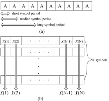
be the normalized CFO with respect to the subcarrier spacing , where is the OFDM symbol period, is the in-teger part of , while is the fractional part. Schmidl and Cox (SC) [5] used two identical half-period symbols to estimate the fractional part of the CFO and a second full-period symbol that has a special correlation relation with the first pilot symbol to estimate . Lim [11] also proposed a similar method and ex-ploited only two identical half-period symbols to estimate both and . Morelli and Mengali (MM) [6] increased the acquisi-tion range to subcarrier spacing by dividing a symbol into repetitive parts, as shown in Fig. 1(a). Their algorithm has been proved to be better than the SC estimate for yielding a smaller minimum mean-square error (MMSE). In addition, their algorithm needs only one symbol period for computing the CFO. The MM algorithm was further improved by the two-stage method of Minn, Tarasak, and Bhargava (MTB) [10]. Song [7] exploited the same pilot symbol structure and suggested a mul-tistage correlation method to acquire CFO, but performance re-sults were the same as those of Schmidl’s. A simplified version of Song’s estimation method that requires only two correlation steps was proposed by Patel [8].
The performance of these methods, except for the MM and MTB algorithms, depends on the correlation of two half-period identical blocks. MM and MTB used differential phases of the correlations between different pairs of adjacent fractional-pe-riod blocks to form an improved CFO estimate.
The blind schemes, on the other hand, exploit the structural and statistical properties of the transmitted OFDM signals such as cyclic prefix [3], virtual subcarrier [4], or constant-modulus [15]. Since no training symbols are required, blind methods are
Fig. 1. (a) Short pilot symbol sequence of the IEEE 802.11a. (b) Symbol arrangement and definitions of the proposed ML estimate.
attractive for saving bandwidth and having higher throughput and are more suitable for circuit-switched transmissions.
In this paper, we present ML CFO estimates that use an arbitrary number of identical fractional-period OFDM blocks. An efficient algorithm is provided to solve the asso-ciated highly nonlinear ML equation. Instead of searching within the candidate CFO range exhaustively, we only need to solve a polynomial of degree . Two methods to further reduce the complexity of extracting the desired root are presented. Numerical results indicate that even at low SNR the performance of the proposed methods still approach the corresponding Cramér–Rao lower bound.
The rest of this paper is organized as follows. Section II scribes our signal model and defines related parameters. We de-rive the corresponding optimal frequency-offset estimate and its simplified version in Section III and Appendix I. A detailed per-formance analysis is presented in Section IV and Appendix II. We discuss the simulation results in Section V and, finally, in Section VI, we summarize our main results.
II. SIGNALMODEL ANDPARAMETERS
Parallel transmission of a block of data symbols drawn from a quadrature-amplitude modulation (QAM) or phase-shift keying (PSK) constellation is efficiently im-plemented by an -point inverse discrete Fourier transform (IDFT). The transformed block of (time-domain) samples
forms a long OFDM symbol, where the equally spaced data-bearing subcarriers are mutually orthogonal over a symbol interval of seconds, where is the IDFT output sample interval. Oftentimes, an OFDM symbol is
pre-ceded by a cyclic prefix longer than the maximum channel delay spread to form an “extended” symbol so that ISI can be elimi-nated at the receiving end by simply discarding the prefix part. One can also have a short OFDM symbol whose duration is a fraction of by placing data symbols only at the subcarriers , i.e., data sequence is transmitted at the frequencies which are multiples of while zeros are inserted at the re-maining frequencies [6].
Let be the th sample of the th (time-domain) short pilot symbol and assume that the preamble part of a transmitted package consists of identical short pilot symbols with a total preamble duration of seconds. We thus have
the relation for and
. Shown in Fig. 1(a) is the IEEE 802.11a
standard that uses , , and to form a
training sequence of ten identical short symbols.
Consider a frequency-selective channel with a maximum delay spread shorter than a short symbol duration. Assuming that the combined frequency response of the prefilters is flat
within the range , where is the signal
bandwidth and is the maximum frequency offset, the received baseband waveform is matched-filtered and sampled at a rate of samples/s. After discarding the first symbol, the remaining received pilot symbols can be repre-sented as
(1)
for , and , where
are uncorrelated circularly symmetric Gaussian random
vari-ables (rvs) with zero mean and variance .
is the channel output corresponding to the transmitted pilot symbol . Due to the assumption that the channel delay spread is shorter than the length of one short symbol and the channel impulse response remains the same during the pre-amble period, the remaining samples are periodic. Note that the above signal model implies that the maximum CFO one can recover is subcarrier spacings.
Define the two vectors
(2) and
(3) where denotes the matrix transpose. Then, as shown in Fig. 1(b), we have
(4)
where , and
. The received samples can thus be expressed compactly as
(5)
where , , and
vectors , we have to estimate through the deterministic vector . For notational simplicity, we shall drop the ar-gument in in the subsequent discussion.
The above signal model (5) assumes that perfect symbol timing has been established prior to frequency synchroniza-tion. However, it is still valid even if timing error does exist provided that the selected received pilot symbols are within the range of the preamble and the number of identical short pilot symbols is larger than (excluding the first discarded received short symbol). Therefore, the beginning position where the received pilot symbols are selected to form the signal is very flexible. More specifically, even if we do not have the symbol timing, we still can use the above signal model provided that the selected short symbols are located within the legitimate interval that spans from the start of the second received short symbol to the last sample of the last transmitted short pilot symbol. Thus, the CFO estimators derived from (5) are expected to be insensitive to timing error.
III. ML ESTIMATE OFCFO
Since the noise is temporally white Gaussian, is a multi-variate Gaussian distributed random vector with covariance ma-trix , where is the identity matrix. The joint ML estimates of and , treating as a deterministic unknown vector, are obtained by minimizing the joint probability density function
(6) The corresponding log-likelihood function, after dropping con-stant and unrelated terms, is given by
(7)
For a given , setting , where
denotes complex gradient operation with respect to , we obtain the conditional ML estimate
, where and denotes the Hermitian
operation. Substituting the least-square solution into (7), we obtain
(8) where denotes the trace of a matrix [18],
, and . Note
that the th entry of the matrix , , is
the correlation value of th and th received symbols,
i.e., . As is
the (time-averaged) autocorrelation matrix of the received
sample vectors , it is a Hermitian matrix such that , where denotes the complex conju-gate. The desired CFO estimate is then given by
(9) It can be proved that the above ML solution is the same as [9, eq. (9)] whose computing load, however, is much heavier. Although (9) gives a compact representation of the ML CFO estimate, it requires an exhaustive search over the entire uncer-tainty range. The resulting complexity may make its implemen-tation infeasible.
We observe, however, that has a special structure that can be of use to reduce the complexity of searching the desired CFO solution of (9). Invoking an approach similar to that used by the
MUSIC algorithm [16], we set and define the
parametric vector
(10) so that the log-likelihood can be expressed as a polynomial of order as follows:
(11)
where , for , and
. To highlight the usefulness of this important ob-servation, we restate it in the form of the following proposition. Proposition 1: The log-likelihood function for a candidate CFO is given by
(12) Some remarks about this proposition are in order.
Remarks:
R1. is the summation of diagonal entries of and is also equivalent to the aperiodic autocorrelation value of the waveform
at time difference seconds, i.e., .
R2. It can be shown that, in the absence of noise
(13)
where , and
. When noise is present, the mean value of is the same as its noise-less value except for ; more specifically,
, where is the
Kronecker delta function. Evaluating (11) at the
unit circle , we obtain the
which has an envelope similar to whose maximum value is at the correct “modified” frequency
.
R3. Due to the Hermitian nature of , is a con-jugate symmetric sequence of length . The symmetric property of guarantees that its Fourier transform is real and nonnegative. This also follows from the semi-positive definiteness of
the quadratic form . Because and
the log-likelihood function constitute a Fourier trans-form pair, we will henceforth refer to as the log-likelihood spectrum or spectrum, for short, and the polynomial defined by (11) the spectrum polynomial.
R4. constitutes a set
of sufficient statistic for estimating . Almost all pre-vious correlation-based algorithms use only a subset of , e.g., For , the Moose’s algorithm [2] uses , the GM algorithm [7] uses . The MM and MTB algorithms use only the phases of elements of . Furthermore, the former achieves its best performance when it uses only half of the phases [10]. It is expected that an algorithm that uses the sufficient statistic would outperform those that use only a part of the sufficient statistic.
R5. Computing the desired CFO estimate through (11) is equivalent to searching for the peak of the candidate spectrum . Hence, the spectrum can be com-puted using a discrete Fourier transform (DFT), but the resolution of the CFO estimate depends on the size of the DFT. Padding more zeros in the sequence results in higher resolution at the expense of inducing higher computation complexity.
As the spectrum is a real smooth function of , taking
a derivative of with respect to and setting
, we obtain
(14)
where is a polynomial of order .
As mentioned before, in a noiseless environment, , the Fourier transform of , is a scaled version of the function , and all roots of
are on the unit circle. The presence of noise and multipath will modify the Fourier transform and move some roots away from the unit circle so that the solutions of become a proper subset of those of . In
that case, we have , where
is a complex constant, , , and
, . Although has a fixed
number of roots, the distribution of these roots among or, equivalently, the degrees of and depend upon SNR for the existence of nonunit-amplitude roots due to the merging of neighboring sidelobes of , which, in turn, results from large noise perturbation.
We can either restrict our search to those roots that are on the unit circle or normalize those nonunit-amplitude roots. Several reasons convince us that both approaches will most likely give the same estimate. First, the desired root is associated with the
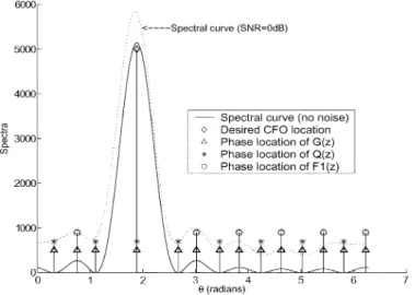
Fig. 2. Normalized log-likelihood spectrum and the associated root distribution where the spectrum is normalized by the noiseless mainlobe peak value; CFO= 1:2 subcarrier spacings.
peak of and the mainlobe-peak-to-sidelobe-peak ratio is greater than 25 dB. As the relative height difference between any two neighboring sidelobe peaks is far smaller than that be-tween the mainlobe and its two neighboring sidelobes, it is much more likely for the merging of neighboring sidelobes than that of the mainlobe and one of its neighboring sidelobes and, even if the latter merge occurs, the associated peak will most probably be the peak of the spectrum. In other words, the desired root is likely to stay at the unit circle with a very high probability. Second, our simulation has shown that, even in the presence of strong noise and severe multipath, the resulting still bears a close resemblance to a scaled version of and the roots on the unit circle are within small neighborhoods of their noiseless locations; see Fig. 2. Finally, is a linear trans-form of and, as (B8) indicates (see Appendix II), can be decomposed into two deterministic terms and two zero-mean complex perturbation terms that are uncorrelated with the deterministic part.
For simplicity, we shall use the first approach, i.e., the desired estimate is to be obtained by
(15) where
(16) Note that we have converted the exhaustive search problem of (9) to a root-finding problem, reducing the candidate solution number from infinity to at most .
A. A ML CFO Estimation Algorithm
We summarize the procedure leading to (16) as follows. 1) Collect received symbols and construct the sample
cor-relation matrix .
2) Calculate the coefficients of based on . 3) Find the nonzero unit-magnitude roots of (14). 4) Obtain the CFO estimate from (15) and (16).
We will refer to the above procedure as Algorithm . It can be shown that, when , the resulting estimate is equivalent to the Moose estimate [2].
The above algorithm needs to locate all of the roots of . We can reduce the order of by truncating the length of the sequence , i.e., using a lesser number of autocorrelation values. When we use the truncated version, , to carry out Algorithm , the resulting algorithm is referred to as Algorithm . The complexity of Algorithm is much less than that of Algorithm since the associated has closed-form solutions. We do expect some performance degradation as less autocorrelation values are used. In the following subsection, we present a method to further reduce the complexity of solving (14) in step 3) with little or no performance degradation.
B. A Simplified CFO Estimate
We notice that the solutions of (14) are the nonzero roots of the polynomial
(17) On the other hand, (14) implies that the roots of satisfy
the equation , where is the imaginary
part of . This observation indicates that the nonzero roots
of (the root of is undesired)
are a subset of the roots of . When is an
arbitrary polynomial, its roots are not necessarily a subset of those of the corresponding defined by (17). However, in our case, as shown in Appendix I, both and do divide
when there is no noise in the received signal vector
or the ensemble average is used to construct
and , i.e., the roots of are indeed a subset of those of . Moreover, we can show (see Appendix I) that the following proposition holds.
Proposition 2: In the absence of noise, the polynomial de-fined by (17), , can be decomposed into
(18) where the desired CFO estimate is one of the roots of defined by
(19)
where .
When noise is present, the above equality becomes an ap-proximation only. Nevertheless, the desired CFO estimate can still be derived immediately from taking the th root of . Fig. 2 highlights the locations of the normalized roots of , and for , i.e., various local extremes of . The global maximum that colocated with a root of corresponds to the desired CFO estimate while the remaining roots of locate at a local minimum (null) of the spectrum. On the other hand, the roots of are at the local sidelobe peaks of the spectrum. It is clear that the union of the roots of and is the set of the roots of . Hence, the com-plexity of extracting the roots is significantly reduced, for we only have to solve the equation , which happens to
have a closed-form expression for its roots. We will show later via simulations and analysis (see Appendix II) that (18) is a valid approximation that incurs only negligible performance loss even when the system is operating at an SNR as low as 0 dB. The above discussion suggests the following simplified CFO esti-mate algorithm.
1) Follow 1) of Algorithm .
2) Compute the coefficients based on two correlation
values and .
3) Solve for the unit-magnitude roots of ,
.
4) Find the estimate from (15) and (16).
The above algorithm will be referred to as Algorithm . Note that the definition of [see (13)] indicates that
and suggests that steps 3) and 4) of Algorithm can be replaced
by using the estimate , where is the
principal value of the argument of . The disadvantage of this es-timate is that it cannot be applied to the situation when the CFO is such that . On the other hand, (13) also implies that
the CFO can be estimated by ,
. Amongst these candidate estimates, is the only one that does not violate the no-phase-am-biguity requirement and, in fact, is the same as the general-ized Moose (GM) algorithm that uses averaged autocorrelation values [7].
IV. PERFORMANCEANALYSIS
Note that the CFO estimate derived from Algorithm is identical to (9). This estimate is unbiased, for as ,
, with
, , and is the channel
response at the subcarrier , hence . In
Ap-pendix II, we show that the variance of the ML estimate is given by
(20)
where . Following the analysis that
leads to [16, eq. (4.1)] and upon substituting the parameter, , we obtain the corresponding Cramer–Rao bound (CRB)
CRB (21)
Equation (20) indicates that is a decreasing function of . Therefore, replacing one long pilot symbol with several identical short symbols and using the proposed ML method would yield a performance superior to that resulting from using the correlation-based method that correlates two identical half-period symbols ( , i.e., Moose algorithm), even though both use the same number of data samples.
For Algorithm , the associated variance can be approx-imated by (22), shown at the bottom of the next page (see Appendix II). Equation (22) reveals that, even at low SNRs, Algorithm still gives a satisfactory performance. For Algo-rithm , we expect its performance to be between those of
Algorithms and , since the former uses all of the available autocorrelation values while one of the two autocorrelation values the latter uses is , which involves a smaller number of time-correlation samples than and is, therefore, less reliable. The simulation results shown in Section V do confirm this conjecture.
It is also clear that, as long as the true CFO does not incur phase ambiguity (i.e., ), then the th roots of are
given by , . Although
in a noiseless environment
(assuming, without loss of generality, the desired root is ), the variance analysis presented in Ap-pendix II shows that yields a smaller variance. As a result, Algorithm yields a performance superior to that of the generalized Moose (GM) estimate obtained by averaging over two consecutive overlapped median symbols [see Fig. 1(a)] times. Later simulation results indeed reveal the supe-riority of Algorithm . Furthermore, it also suggests that step 4) can be replaced by picking up the th root whose principal
argument is closest to .
V. SIMULATIONRESULTS ANDDISCUSSION
Numerical examples are provided in this section to examine the behavior of the proposed CFO estimation technique. As shown in Fig. 1(a), eight short training symbols which are the same as those used in the IEEE 802.11a preamble are used in our simulation. Results reported in Figs. 3–6 assume a static frequency-selective fading channel with ten paths whose com-plex amplitudes are independent identically distributed (i.i.d.) complex Gaussian random variables. CFO is normalized by sub-carrier spacing and the mean values and mean-squared errors (MSE) of various estimates are computed by independent trials.
For comparison purposes, the corresponding CRBs and the behaviors of four other estimates are provided as well. These estimates are the MTB estimate (which outperforms the MM estimate [10]), the Moose estimate [2], the GM estimate, and the Patel–Song [7], [8] (PS) estimate. The last estimate uses the GM estimate as the initial estimate and selects the final estimate
from the family of candidate estimates ,
where is the Moose estimate and is the set of integer multiples of twice the acquisition range of that is the closest to the initial estimate. The GM estimate is a special case of our proposals, corresponding to one that uses the truncated
version of the spectrum polynomial, .
The GM estimate has a frequency acquisition range larger than that of the Moose estimate but renders a less accurate estima-tion when CFO is within the latter’s acquisiestima-tion range. The PS estimate is designed to retain the advantages of both algorithms,
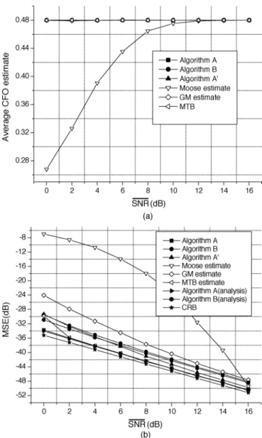
Fig. 3. (a) Averaged estimation values for various CFO estimates. (b) MSE performance of CFO estimates;K = 8, and true CFO = 0:48 subcarrier spacings.
i.e., having an acquisition range the same as that of the GM es-timate while achieving the performance of the Moose eses-timate. The coefficients used by the MTB estimate to optimally com-bine the differential phases of the elements in the set depend on the operating SNR. In our simulation, a design 20 dB is assumed. The MM estimate is not compared for it best per-formance is achieved when only correlations are used [10]. For the purpose of fair comparison, all algorithms whose per-formance is shown in the same figure use the same number of samples.
Fig. 3(a) and (b) depicts the mean and MSE of various CFO estimates as a function of SNR. Since the maximum CFO that can be corrected by the Moose estimate is , the
Fig. 4. MSE performance of CFO estimates;K = 8, and true CFO = 1:8 subcarrier spacings.
corresponding performance degrades rapidly at low SNR when the true CFO approaches the maximum correctable value. For Algorithms , , and and the MTB and GM estimates, however, the maximum correctable CFO is , hence they give a much better MSE performance with Algorithm yielding a performance almost the same as that of the CRB. Both Algorithms and (corresponding to ) outperform the Moose (corresponding to ) and GM estimates. For 802.11a systems, using eight short training symbols not only allows a larger CFO offset range but also yields better performance. At CFO , as shown in Fig. 3, the Moose estimate is worse than the GM estimate at low SNRs. Algorithm is simpler but its performance is a little worse than those of Algorithms and , though it is still better than the GM estimate at low-to-medium SNRs. The performance of the MTB estimate is almost the same as that of Algorithm A except at low SNR.
Fig. 4 plots the MSE performance for CFO . Algo-rithms and and the MTB estimate still maintain superior performance in this case. For the MTB estimate, however, the effects of SNR mismatch and initial CFO estimation error be-come apparent at low SNRs. Fig. 5 plots the MSE performance when CFO using four short symbols. The Moose es-timate uses two identical symbols: each lasts for short symbol durations so that the maximum offset range it can correct becomes . Fig. 6 compares the MSE performance of our algorithms and the GM and PS estimates when CFO . Figs. 5 and 6 clearly indicate that the PS (or Moose) estimate is not necessarily better than the GM estimate but that the pro-posed methods still provide the best performance although the improvement is less impressive. This confirms our analysis in Section IV where it is shown that the performance of Algorithm improves as increases. Finally, we examine the perfor-mance in a time-varying channel composed of ten uncorrelated fading paths generated by the modified Jakes’ model [17]. The maximum path delay is equal to ten data sample intervals, as-suming a sampling rate of 20 MHz. The performance of our CFO estimates is independent of the path numbers so long as
Fig. 5. MSE performance of CFO estimates;K = 4, and true CFO = 0:94 subcarrier spacings.
Fig. 6. MSE performance of CFO estimates;K = 4, and true CFO = 1:6 subcarrier spacings.
the channel’s maximum delay spread is shorter than the length of the cyclic prefix. Assuming a mobile speed of 100 km/h, cor-responding to a Doppler frequency of approximately 463 Hz when the carrier frequency is 5 GHz, we plot the corresponding MSE performance in Figs. 7 and 8. As our derivations assume a quasi-static channel that remain unchanged during the preamble period, the estimation performance is degraded due to the fact that the received signal model (4) is no longer valid. In sum-mary, Algorithms and and the MTB estimate render the best performance, followed by Algorithm , and then the other correlation-based algorithms. When is small, Algorithms , , and yield almost the same MSE performance. The pro-posed methods can be used when an arbitrary number of identical pilot symbols are available.
As for the computational complexity issue, we first noticed that the basic requirement is the computing of . Different methods call for the computation of different subsets of the sufficient statistic . The detailed computational complexity
Fig. 7. MSE performance of CFO estimates in a time-varying frequency-selective Rayleigh fading channel;K = 8, and true CFO = 1:8 subcarrier spacings.
Fig. 8. MSE performance of CFO estimates in a time-varying frequency-selective Rayleigh fading channel;K = 4, and true CFO = 1:6 subcarrier spacings.
and storage requirement for the CFO estimation algorithms are listed in Table I, assuming that there are short pilot symbols available with each symbol of -sample duration. Clearly, Algorithm and the MTB estimate require the highest complexity while Algorithm is the simplest among the three proposed algorithms. The MTB algorithm needs to perform down-converting (multiplying exponentials) that require table loop-ups. The storage requirement for building the table is not included in Table I. The computing effort for finding the roots is also not included. Algorithm needs one additional real division only. Algorithm has to solve a polynomial of order four that renders a closed-form expression while Algorithm has to solve a polynomial of order , and the associated complexity is relatively high. A method to significantly reduce this complexity can be found if one uses the phase of as
the initial phase value for searching for the roots. An elemen-tary root-finding algorithm like Newton’s method can then be applied to find the first unit-magnitude root of in just a few iterations, as the desired root has a phase very close to that
of .
VI. CONCLUSION
The optimal ML CFO estimate that uses several identical pilot symbols has been derived. By transforming the log-likelihood function into a spectrum polynomial, we reduce the ML estimate’s complexity from that of an exhaustive search over a continuum to that of solving a polynomial. Besides the ML estimate (Algorithm ), we propose two simplified versions (Algorithms and ) and show that some of the previous correlation-based algorithms are special cases of our proposals. The MSE performance of the proposed algorithms are analyzed in detail, and our analysis does match the simulation results. Both the analysis and simulations indicate that the performance of Algorithm is very close to the corresponding CRB. Algorithms and require much less computational load but they do not incur a noticeable loss of performance. Numerical results also demonstrate that, in a time-varying Rayleigh fading channel, the performance of the proposed methods suffers from minor performance degradation only.
APPENDIX I
DERIVATION OF(18)AND THEROOTDISTRIBUTION OF
Dividing by , we obtain the quotient polynomial defined by (19) and the remainder polynomial
(A1)
where ,
. In the
ab-sence of noise, we have with
. Invoking the definition and substituting the resulting
alter-native expressions , , and
, for , we
find that for . Therefore, and
the polynomial are indeed a factor of . Similarly, it is easy to see that, if the ensemble average is used to construct and , we still have the factorization (18).
Obviously, the roots of the quotient polynomial
are the set ,
which has the desired root as one of its members. Next we prove that the other roots of are located at the sidelobes
TABLE I
COMPLEXITYCOMPARISON OFVARIOUSCFO ESTIMATIONALGORITHMS
of the log-likelihood spectrum . Recall that . Assuming is even, we obtain
(A2)
It is obvious that if , for
. Hence, when , for
, which are the remaining roots of . The case is odd can be similarly proved. Note that the roots of are the extreme values of the spectrum of . Since the roots of are located at either the global maximum or the local minima of , the roots of should sit at the local maxima, i.e., sidelobe peaks of the spectrum, as shown in Fig. 2. The above discussion assumes a noiseless environment. When noise is present, we can easily show that the factorization of still holds in the mean sense. Furthermore, the analysis of presented in Appendix II convinces us that factorization (18) will remain valid with a probability close to one unless SNR is very small (say, 0 dB).
APPENDIX II
MSE PERFORMANCEANALYSIS
A. Decomposition of the Correlation Coefficients
The performance of the proposed algorithms depends on the behavior of whose coefficients , as shown in R2 of the main text, are functions of the autocorrelation matrix . We thus begin our anal-ysis by examining
(B1)
where . Let be the
discrepancy matrix between and its ensemble
av-erage, , i.e., .
It can be shown that , where
, and the discrepancy matrix consists of three components
(B2)
where ,
.
The first component, , is independent
of SNR and the CFO estimation algorithm. Using the
definition , we
ex-press the second component as the sum of two matrices , where the entries of the second matrix are given by while the first matrix is a diagonal matrix. The third component, , represents the cross correlation of the received samples and noise. We will show that only and affect the mean-squared performance of our CFO estimates.
We first note that the assumption that are i.i.d. zero-mean Gaussian rvs with variance leads immediately to for , and then the equations
(B3) for
(B4)
for , and for .
Furthermore, it can be shown that all of the elements in the upper or lower triangular part of are zero mean uncorrelated rvs
with identical variance and .
Therefore, the rvs
have zero mean and variances for
. Moreover, , , and
is a sequence of uncorrelated rvs. Next, let us examine the statistical properties of .
Recall that
, whose entry is given by
(B6)
with . It follows immediately that
, for is assumed to be uncor-related with , for all . Equation (B6) thus gives , for . Similarly, we can show that the entries of the cross-correlation matrix are uncorrelated unless they belong to the same column or row in the upper (or lower) triangular part of .
In other words, , for ,
and , for , but
, for ,
and , for
. The new zero-mean rvs
(B7)
have variances for and the
Hermi-tian property but they are not independent. Now we can express the sequence as
(B8)
Note that , , and are uncorrelated.
B. Performance of Algorithm
As Algorithm calls for locating the point (or ) that
max-imizes (or ), it follows that ,
where . Assuming
small estimation errors , we obtain
, where and .
The fact that implies , and thus
the estimation error can be approximated by
(B9) The statistical properties of and derived in the previous section convince us that, with high probability, , if 0 dB. Ignoring the perturba-tions due to and in the denominator, we can further simplify (B9) to
(B10)
where is a zero-mean rv.
Thus, the MSE of the estimate can be obtained as soon as the second moment of is known.
Invoking the alternate expression
and the facts that and are uncor-related and is white but not , we obtain
(B11) where is the sum of the cross-correlation value of corre-lated elements ’s, i.e.,
(B12) As mentioned in Appendix II-A,
and for
, after some algebra, we can show that the first term on the right-hand side of (B11) is equal to
(B13) The value of remains to be determined. For convenience, we define the auxiliary rv
(B14)
for , , and . If , the
associ-ated rv is zero with probability 1. It follows that entries of the upper triangular matrix are uncorrelated unless they belong to the same row or column. In other words,
for and
for , but
for and
for . By using (B7), (B12), and (B14), we can prove that is equivalent to the sum of cross correlations of the entries of , i.e.,
(B22)
where denotes the “exclusive or” operator. As , , and the recursive relation
(B16) holds for , we obtain
(B17) This equation, along with (B10), (B11), and (B13), yields
(B18)
The relation then leads to
(B19)
C. Performance of Algorithm
Algorithm calls for solving or, equivalently, the
evaluation of the corresponding roots ,
. Since ,
, and
, it is convenient to
define intermediate rvs and
(whose variances are given by
and ,
respec-tively) so that we can write
(B20)
where and . Note that and are
corre-lated but their correlation is a decreasing function of and their
variances are and ,
respectively. After some algebra, we obtain
(B21)
where . It can be shown that
, the variance of , is given by (B22), shown at the top of the page. However, if we assume that and are uncorrelated,
the corresponding variance of , denoted by is simply , given by
(B23) Numerical results show that the difference between and is about 1 dB within the range of interest.
Equation (B21) implies , and the
polar coordinate representation gives
(B24) where and are the amplitude and phase of ,
re-spectively. When , i.e., and ,
we have
(B25)
where we have used the approximation , for
. Hence, the variance of can be obtained from . Without loss of gener-ality, we assume that the phase of the desired root of in
(19) is , then the CFO estimate
becomes
, and, as a result, by substituting , we obtain the variance of the estimate (22) as
(B26)
REFERENCES
[1] J. Terry and J. Heiskala, OFDM Wireless LANs: A Theoretical and
Prac-tical Guide. Indianapolis, IN: Sams, 2001.
[2] P. H. Moose, “A technique for orthogonal frequency division multi-plexing frequency offset correction,” IEEE Trans. Commun., vol. 42, pp. 2908–2914, Oct. 1994.
[3] F. Daffara and O. Adami, “A novel carrier recovery technique for or-thogonal multicarrier systems,” Eur. Trans. Telecommun., vol. 7, pp. 323–334, July/Aug. 1996.
[4] H. Liu and U. Tureli, “An high-efficiency carrier estimator for OFDM communation,” IEEE Commun. Lett., vol. 2, pp. 104–106, Apr. 1998. [5] T. M. Schmidl and D. C. Cox, “Robust frequency and timing
synchro-nization for OFDM,” IEEE Trans. Commun., vol. 45, pp. 1613–1621, Dec. 1997.
[6] M. Morelli and U. Mengali, “An improved frequency offset estimator for OFDM applications,” IEEE Commun. Lett., vol. 3, pp. 75–77, Mar. 1999.
[7] H.-K. Song, Y.-H. You, J.-H. Paik, and Y.-S. Cho, “Frequency-offset synchronization and channel estimation for OFDM-based transmission,”
IEEE Commun. Lett., vol. 4, pp. 95–97, Mar. 2000.
[8] S. Patel, L. S. Cimini, and B. McNair, “Comparison of frequency offset estimation techniques for burst OFDM,” in Proc. 55th IEEE Vehicular
[9] J. Li, G. Liu, and G. B. Giannakis, “Carrier frequency offset estimation for OFDM based WLANs,” IEEE Signal Processing Lett., vol. 8, pp. 80–82, Mar. 2001.
[10] H. Minn, P. Tarasak, and V. K. Bhargava, “OFDM frequency offset esti-mation based on BLUE principle,” in Proc. IEEE Vehicular Technology
Conf., Vancouver, BC, Canada, Sept. 2002, pp. 1230–1234.
[11] Y. S. Lim and J. H. Lee, “An efficient carrier frequency offset estima-tion scheme for an OFDM system,” in Proc. 52nd IEEE Vehicular
Tech-nology Conf., Sept. 2000, pp. 2453–2457.
[12] A. J. Coulson, “Maximum likelihood synchronization for OFDM using a pilot symbol: part 1: algorithms, part 2: analysis,” IEEE J. Select. Areas
Commun., vol. 19, pp. 2486–2503, Dec. 2001.
[13] T. Keller, L. Piazzo, P. Mandarini, and L. Hanzo, “Orthogonal frequency division multiplex synchronization techniques for frequency-selective fading channels,” IEEE J. Select. Areas Commun., vol. 19, pp. 999–1008, June 2001.
[14] L. Piazzo, T. Keller, A. Falaschi, and P. Mandarini, “Time and frequency synchronization in DQPSK-OFDM based high speed wireless local area networks,” Eur. Trans. Telecommun., vol. 13, no. 3, pp. 279–284, May/June 2002.
[15] M. Ghogho and A. Swami, “Blind frequency-offset estimator for OFDM systems transmitting constant-modulus symbols,” IEEE Commun. Lett., vol. 6, pp. 343–345, Aug. 2002.
[16] P. Stoica and A. Nehorai, “MUSIC, maximum likelihood, and Cramér-Rao bound,” IEEE Trans. Acoust., Speech, Signal Processing, vol. 37, pp. 720–741, May 1989.
[17] Y. Li and Y. L. Guan, “Modified Jakes’ model for simulating multiple un-correlated fading waveforms,” in Proc. 51st IEEE Vehicular Technology
Conf., Tokyo, Japan, May 2000, pp. 1819–1822.
[18] G. H. Golub and C. F. VanLoan, Matrix Computations, 3rd ed. Balti-more, MD: Johns Hopkins Univ. Press, 1996.
Jiun H. Yu was born in Nantou, Taiwan, on March
16, 1979. He received the B.S. and M.S. degrees in communication engineering from National Chiao Tung University, Hsinchu, Taiwan, in 2001, and 2003, respectively.
He is currently a System Design Engineer with the Research and Development Center, Realtek Semiconductor Corporation, Hsinchu. His research interests include digital transmission systems, de-tection and estimation theory, and communication signal processing.
Yu T. Su (S’81–M’83) received the Ph.D. degree
in electrical engineering from the University of Southern California, Los Angeles, in 1983.
From 1983 to 1989, he was with LinCom Cor-poration, Los Angeles, where he was a Corporate Scientist, where his work involved the design of various measurement and digital satellite commu-nication systems. Since September 1989, he has been with National Chiao Tung University, Hsinchu, Taiwan, where he was head of the Communication Engineering Department between 2001 and 2003. He is also affiliated with the Microelectronics and Information Systems Research Center of the same university and served as a Deputy Director from 1997 to 2000. His main research interests include communication theory and statistical signal processing.