Polarization and distribution function of the Lambda(b) baryon

Polarization and distribution function of the

⌳

_b

baryon

Tsung-Wen Yeh

Institute of Physics, National Chiao-Tung University, Hsinchu 300, Taiwan 共Received 4 April 2002; published 7 August 2002兲

The polarization of the⌳b baryon has been measured in ALEPH, OPAL, and DELPHI experiments. A significant loss on the transfer of the b quark polarization to the⌳bbaryon polarization has been noticed. This implies that the hadronization effects cannot be neglected. Therefore we may make use of the polarization measurements to look for a suitable model for the⌳bdistribution function. To investigate the⌳bpolarization, we construct four models based on a perturbative QCD factorization formula. The models are the quark model, the modified quark model, the parton model, and the modified parton model. The modified models mean the models having transverse degrees of freedom and the associated soft radiative corrections having been re-summed. The quark and parton models cannot describe all experiments at the same time. On the other hand, the modified models can have the power to explain all data in the same formalism.

DOI: 10.1103/PhysRevD.66.034004 PACS number共s兲: 13.88.⫹e, 12.39.Hg

I. INTRODUCTION

The polarization of bottom baryons ⌳b’s has been mea-sured by ALEPH 关1兴, OPAL 关2兴, and DELPHI 关3兴. The ALEPH data showed that the ⌳b polarization has a value P⫽⫺0.23_⫺0.20⫹0.24(stat)⫾0.08(syst). The OPAL data indicated the polarization P⫽⫺0.56_⫺0.13⫹0.20(stat)⫾0.09(syst). The DEL-PHI experiment gave P⫽⫺0.49_⫺0.30⫹0.32(stat)⫾0.17(syst). Al-though these three measurements are compatible with each other, the ⌳b polarization still has a wide range of value from⫹0.01 to ⫺0.79. To improve the situation, it is better to find out a sensitive measurable quantity on the polarization. However, this is very difficult before we have a more quali-tative understanding on the spin properties of ⌳b baryons. This paper is intended to understand the behind mechanisms by constructing physical models based on perturbative QCD formalism.

Measurement of a large longitudinal polarization of the ⌳b may indicate the polarization of a primary b quark pro-duced from a Z0 decay. The b quarks produced in the reac-tion e⫹e⫺→Z0→bb¯ are highly polarized with polarization P⫽⫺0.94 关4–6兴. The corrections from hard gluon emis-sions and mass effects can change the polarization of the final state b quarks by only 3% 关7,8兴. The b quark can frag-ment into mesons and baryons. The decays of b mesons into spin zero pseudoscalar states do not retain any polarization information. The hadronization to b baryons might preserve a large fraction of the initial b quark polarization. In the heavy quark mass limit, the spin degrees of freedom of the b quark are decoupled from a spin-zero light diquark. The ini-tial polarization of the b quark can therefore be preserved until the ⌳b decays. The higher mass b baryon states can decay into the ⌳b baryon but transfer little spin degrees of freedom. These effects have been estimated from different scenarios as about 30%. This leads to that the final ⌳b po-larization could be P⫽⫺0.6–0.70 关9,10兴.

The ALEPH Collaboration measured the ⌳b polarization by employing the method suggested by Bovicini and Randall 关11兴. In the ratio y(P)⫽

具

El( P)

典

/

具

E␯¯( P)

典

with

具

El

典

and

具

E_␯¯

典

the average lepton and antineutrino energies in the

laboratory reference frame, the fragmentation effects are largely cancelled out. Also, the spectra of the electrons and antineutrinos produced from the inclusive semileptonic de-cays of polarized⌳bbaryons are harder relative to the spec-tra of unpolarized decays. The ALEPH Collaboration pro-posed to measure the ratio R( P)⫽y(P)/y(0), which is a Lorentz invariant quantity. The ⌳b polarization is then ex-tracted from a comparison between the measured ratio RALEPH⫽1.12⫾0.10 and a Monte Carlo simulation ratio RMC( P) with varying P. Because the⌳b polarization is best defined in the rest frame of the⌳_b baryons, one can rewrite the ratio R in terms of the average variables in the rest frame to determine the polarization

P⫽

具

E_l*

典具

E_␯¯*

典

共1⫺R兲

具

E_l*

典具

P_␯¯*

典

R⫺

具

E_␯¯*

典具

P_l*

典

, 共1兲

where the star variables denote the average quantities in the rest frame and are evaluated with P⫽⫺1. Theoretically, the values of average quantities in the above equation are model dependent. They are sensitive to the nonperturbative model employed for calculation. For example, if we apply the free quark model to calculate the star variables, we can obtain the polarization P⫽⫺0.23, which is closed to the ALEPH’s re-sult 关1兴. The situation will become interesting as we apply the same model for the DELPHI experiment. The DELPHI experiment measured the same ratio RDELPHI⫽1.21_⫺0.14⫹0.16and obtained PDELPHI⫽⫺0.49_⫺0.30⫹0.32. In the same way, it is easy to check that substituting DELPHI’s ratio RDELPHIinto Eq.共1兲 can derive a different value P⫽⫺0.38 in the free quark model. On the other hand, in the same model, if we employ the OPAL’s polarization POPAL⫽⫺0.56 into the ALEPH’s and DELPHI’s Monte Carlo simulation ratios RMC, we can extract the central value of corresponding R as R1⫽1.30 and

R2⫽1.27, respectively. This seems to imply that there

re-quires more investigations to find a consistent picture for⌳b polarization. That is we need to find a model which can explain the experiments self-consistently. The model

depen-dence in the equation for P, such as Eq.共1兲, arises from the z variable zl(␯¯)⫽

具

P_l(*_␯¯)

典

/

具

E_l(*_␯¯)

典

. Using the z variables, Eq. 共1兲 can be recast as

P⫽ 共1⫺R兲 z_␯¯R⫺zl

. 共2兲

It will become clear in the following sections that different models would give different values of ratio zlbut almost the same z_␯¯ due to the characteristics of the lepton and an-tineutrino spectra.

In order to explore the mechanisms controlling the spin properties of polarized⌳_bbaryons, we shall investigate four models. They are the共free兲 quark model 共QM兲, the modified quark model共MQM兲, the parton model 共PM兲, and the modi-fied parton model 共MPM兲. The parton model describes the probability of finding the b quark carrying a momentum frac-tion of the momentum of the ⌳b baryon by a parton distri-bution function. The quark model assumes that the ⌳b baryon contains only one b quark and two light quarks and the corresponding parton distribution function is just a delta function of the momentum fraction. This means that the b quark carries almost all the ⌳b baryon momentum. The modified quark model and the modified parton model mean that the quark model and the parton model contain an addi-tional Sudakov form factor and transverse momentum. The Sudakov form factor arises from a resummation over radia-tive corrections of soft gluons and have the effects to en-hance the perturbative QCD contributions.

We emphasize the importance of transverse degrees of freedom of partons inside a⌳bbaryon in our analysis. First, the transverse momenta regularize the divergences when the outgoing c quark in the process b→cW is approaching the end point. Second, the transverse momenta also enhance the contributions from the spin vector along the polarization di-rection. For completeness, we also introduce the intrinsic transverse momentum for the distribution function. We as-sume that the form of the intrinsic transverse momentum part of the parton distribution function can be parametrized as exp关⫺tM2b2兴 with an impact parameter b, which is the con-jugate variable of the transverse momentum. The other fac-tors are the ⌳b baryon mass M and a dimensionless param-eter t. The impact paramparam-eter b will be integrated out in our perturbative QCD 共PQCD兲 formalism. The z variables are functions of t. To determine the parameter t we rely on the experiments. The OPAL Collaboration determined the polar-ization by comparing the measured distribution of the ratio E_␯¯/El against a simulation of this ratio using the JETSET Monte Carlo event generator. The polarization POPAL of the OPAL experiment and results of the ALEPH and DELPHI experiments will determine the range of parameter t.

The arrangement of our paper is as follows. In the next section, we shall demonstrate the factorization formula for the inclusive semileptonic decay of the ⌳b baryon. In this formula, the hard scattering amplitude, describing the short distance subprocess b→cl¯ , convolutes with a jet function␯ and a universal soft function. For simplicity, we shall assume that the charm quark mass can be ignored. That is we shall

neglect the corrections like m_c2/ M2with m_cthe charm quark mass. This approximation is less than 10% and is safe as compared with the accuracy of the experiments. However, it requires one to consider the collinear divergences due to our ignorance of the charm quark mass. The jet function is then necessary for absorbing the collinear divergences. The uni-versal soft function involves the b quark matrix element. The matrix element contains a large scale factor, the b quark mass Mb. To have a well established matrix element, we need to employ heavy quark effective theory 共HQET兲 to scale out this large scale. We also need to separate the leading order matrix elements in 1/Mb expansion from the higher order ones. We shall develop a description for separating the lead-ing order from the higher order mass corrections. This de-scription is equivalent to the OPE approach. In Sec. III, we shall construct four models based on the factorization for-mula. Section IV gives the numerical result. The conclusion is given in Sec. V.

II. FACTORIZATION FORMULA

We shall investigate the quadruple differential decay rate for polarized ⌳b baryons,⌳b→Xcl¯ ,␯

d4⌫ dEldq2dq0d cos␪l ⫽兩Vcb兩 2_G F 2 256␲4M L␮␯W ␮␯_{, 共3兲}

where M denotes the mass of the⌳b baryon, L␮␯ represents the leptonic tensor

L_␮␯⫽Tr关P”l⌫␮P”␯¯⌫␮兴, 共4兲 and W␮␯ means the hadronic tensor

W_␮␯⫽共2␲兲3␦(4)共P_⌳ b⫺q⫺PXc兲 ⫻

兺

X

具

⌳b兩c¯⌫ ␮_†b兩X c

典具

Xc兩c¯⌫␯b兩⌳b

典

d3PX_c 共2␲兲3_2E X_c , 共5兲

where⌫␮denotes the V⫺A operator␥␮(1⫺␥5),兩Xc

典

means the hadronic states containing a charm quark, and q is total momentum carried by the lepton and antineutrino. We choose the normalization for the ⌳b state 兩⌳b

典

as

具

⌳b( P_⌳

⬘

_b,S)兩⌳b( P⌳_b,S)

典

⫽(2␲)3(2 P_⌳b

0

)␦3(Sជ⫺Sជ

⬘

)␦3( Pជ_⌳

b

⫺Pជ_⌳

⬘

_b). The kinematical variables El,q,q0, and cos␪l are expressed as follows. We choose the ⌳b baryon rest frame such that the initial⌳bbaryon momentum, P⌳_b, and the final state lepton and antineutrino momenta, pl and p␯¯, can be defined as P_⌳ b⫽ M

冑

2共1,1,0兲,pl⫽共pl ⫹_,0,0兲,p ␯¯⫽共p␯¯⫹, p␯¯⫺,p␯¯⬜兲. 共6兲

The variables E_l,q, and q₀ are related to p_l⫹, p_␯¯⫹, p_␯¯⫺ as E_l ⫽pl⫹/

冑

2,q2⫽2pl⫹p_␯¯ ⫺_{, and q} 0⫽(pl⫹⫹p_␯¯ ⫹_⫹p ␯¯ ⫺_)/

_冑

_{2. We let}

is set as Pb

2_⬇M

b

2

with Mb the b quark mass. The momentum l of the light degree of freedom of the⌳b baryon can have a large plus component and small transverse components l_⬜. The final state charm quark momentum is equal to Pc ⫽P_⌳b⫺l⫺q. The angle ␪l is defined as the angle between the third component of pland that of the b quark polarization vector, Sb. The differential decay rate can also be rewritten in terms of E_␯¯,y ,y0, and␪␯¯with E␯¯the antineutrino energy

and corresponding angle␪_␯¯. Because the right-hand side of Eq. 共3兲 is independent of which parametrization for the lep-tonic variables, we shall use both parametrizations for the differential decay rate.

It is convenient to use the scaled variables xl(␯¯) ⫽2El(␯¯)/ M ,y⫽q2/ M2, and y0⫽2q0/ M . The integration

re-gions for xl(␯¯), y , and y0 are

0⭐xl(␯¯)⭐1, 0⭐y⭐xl(␯¯), y

xl(␯¯)

⫹xl(␯¯)⭐y0⭐1⫹y. 共7兲

Note that we have chosen M as the scale factor. For simplic-ity, we have chosen m_c⫽0 and left m_c⫽0 to other work. This approximation is safe as compared with the accuracy of available experiments. The leading corrections to this ap-proximation are of order O(m_c2/ M_b2) being less than 10%.

By optical theorem, the hadronic tensor W␮␯ can be re-lated to the forward matrix element T␮␯through the formula

W␮␯⫽⫺Im共T

␮␯_兲

␲ . 共8兲

The lowest order of T␮␯ is defined as

T␮␯⫽⫺i

冕

d4y eiq•y

具

⌳_b兩T 关J†␮共0兲,J␯共y兲兴兩⌳_b

典

共9兲 with J␮⫽q¯␥␮(1⫺␥5)b the V⫺A current. We have

abbrevi-ated the state vector 兩⌳b( P⌳_b,q,S)

典

as 兩⌳b

典

. The forward matrix element can be expressed in the momentum space

T␮␯⫽⫺i

冕

d 4_P b 共2␲兲4 Tr关S ␮␯_共P b⫺q兲T共Pb兲兴, 共10兲 where the trace is taken over the fermion indices and color indices, the hard function S␮␯( P_b⫺q) describes the short distance decay subprocess, b→Wc, and the soft function T( P_b) denotes the long distance matrix element

T共Pb兲⫽

冕

d4y ei Pb•y

具

⌳b兩b¯共0兲b共y兲兩⌳b

典

. 共11兲 Because we are only interested in the leading contributions in this note, we are required to separate the leading contri-butions from subleading contricontri-butions. To specify the leading contributions, we also need to consider correction terms. The correction contributions may come from radiative correction terms like ␣_sn and power correction terms like 1/Mm for

n,m⭓1. Among the radiative corrections, the contributions from soft gluons will become dominant at the end points, at which the final state quark is approaching on-shell. As dis-cussed in the Introduction, the hard gluon emissions can only contribute about 3%. Therefore we shall retain the soft gluon contributions at the end points. To discuss the power correc-tion terms, we need to be more careful. As investigated in the operator product expansion共OPE兲 and heavy quark effective theory 共HQET兲 approach, the power corrections can have two sources; one from the short distance expansion for the forward matrix element and the other one from the heavy quark mass expansion for the expanded matrix elements. Here, we shall present a different approach in which the leading order matrix elements are in terms of nonlocal heavy quark currents composed of heavy quark effective fields in HQET.

We now demonstrate this description. To start up, we ex-press the forward matrix element

iT␮␯⫽

冕

d 4_P b 共2␲兲4Tr关S ␮␯_共P b⫺q兲T共Pb兲兴 ⫹

冕

d 4_P b 共2␲兲4

冕

d4P_b

⬘

共2␲兲4 Tr关S␣ ␮␯_共P b⫺q,Pb

⬘

⫺q兲 ⫻T␣_共P b, Pb

⬘

兲兴⫹••• 共12兲

by including a higher order term from triple parton matrix elements containing gluon fields

T␣共Pb, Pb

⬘

兲⫽

冕

d

4_y

冕

_d4_zei P_b•y_ei( P_b⫺P_b⬘)•z

⫻

具

⌳b兩b¯共0兲关⫺gA␣共z兲兴b共y兲兩⌳b

典

共13兲 with A␣(z) the gluon fields. The P_b and P_b

⬘

denote the out-going and incoming b quark momenta. The hard functions S␮␯ and S_␣␮␯ have the following expressions:

S␮␯⫽⫺⌫ ␮_P” c⌫␯ P_c2⫹i⑀ , 共14兲 S_␣␮␯⫽ ⌫ ␮_P” c␥␣P”c

⬘

⌫␯ 共Pc 2_{⫹i⑀兲共P} c

⬘

2_⫹i⑀兲, 共15兲

where Pc( Pc

⬘

)⫽Pb( Pb

⬘

)⫺q. We shall employ the light-cone gauge A⫹⫽n•A⫽0. To continue, it is useful to introduce the light-cone vectors p and n in the⫹ and ⫺ directions, respec-tively. These two vectors satisfy properties p2⫽n2⫽0 and p•n⫽P_⌳

b•n. The ⌳b baryon momentum P⌳b is then recast

as P_⌳ b ␮ _⫽p␮_⫹ M 2 2 p•nn ␮_{. 共16兲}

For the b quark inside the ⌳b baryon, we parametrize its momentum P_b as

Pb␮⫽zp␮⫹ Pb 2_⫹P b_⬜ 2 2 Pb•n n␮⫹Pb␮_⬜ 共17兲 ⫽Pˆb␮⫹ Pb 2_⫺M b 2 2 Pb•n n␮, 共18兲 where Pˆb 2_⫽M b 2

is the on-shell part of Pb and the momentum fraction z defined by z⫽P_b⫹/ P_⌳

b

⫹_⫽1⫺l⫹_{/ P} ⌳b

⫹ _{. By the}

pa-rametrization of Pb, the b quark propagator is then ex-pressed as i P”_b⫺M_b⫹i⑀⫽ i共P”ˆb⫹Mb兲 P_b2⫺M_b2⫹i⑀⫹ in” 2 Pb•n⫹i⑀ ⬅Fb L_共P b兲⫹Fb S_共P b兲. 共19兲

There are two scenarios to be discussed. The first situation is for small z. That is we allow l⫹ to be of order P_⌳

b

⫹ _{and z} ⬃⌳/M with ⌳⬃⌳QCD. The Fb

S

( Pb) term having power like 1/⌳ is as important as the F_bL( Pb) term. We shall see later that the power correction completely comes from the short distance hard function. There is also the second situation in which the value of z is large of order 1⫺⌳/M. This corre-sponds to small l⫹. In this case, the F_bS( Pb)⬃1/M is power suppressed than Fb

L

( Pb)⬃1/⌳. In this configuration, the hard function is in the end points x→1 and y→0,y0→1. The

power corrections come from the noncollinear momentum of the b quark. We now investigate the contributions from the above two scenarios. For simplicity, we shall ignore the transverse component of the neutrino momentum. This will not affect the following analysis.

For the large l⫹scenario, we need to separate the leading terms of the hard functions S␮␯,S_␣␮␯ from the higher order terms. The hard function S␮␯ is a function of l and S_␣␮␯ a function of l and l

⬘

. The l and l

⬘

are momenta of light de-grees of freedom of the ⌳_b and are defined as l⫽P_⌳

b⫺Pb

and l

⬘

⫽P_⌳

b⫺Pb

⬘

. We can make Taylor expansion for S

␮␯

and S_␣␮␯ with respect to l⫹ and l⫹

⬘

. This is because the momentum l(l

⬘

) have a large plus component l⫹⫽␰p(l⫹

⬘

⫽␰

⬘

p) with␰⫽1⫺z(␰

⬘

⫽1⫺z

⬘

). By performing Taylor ex-pansions for S␮␯(l) and S_␣␮␯(l,l

⬘

) around S␮␯(␰p) and S_␣␮␯(␰p,␰

⬘

p), we then obtain S␮␯共l兲⫽S␮␯共␰p兲⫹⳵S ␮␯ ⳵l␣

冏

l⫽␰p 共l⫺␰p兲␣⫹•••, 共20兲 S_␣␮␯共l,l

⬘

兲⫽S_␣␮␯共␰p,␰

⬘

p兲⫹••• . 共21兲 The following low energy theorems are assumed to hold

⳵S␮␯

⳵l␣ 共␰p兲⫽⫺S␣

␮␯_{共␰p,␰p兲. 共22兲}

The minus sign in the above equations is due to the direction of the momentum flow of l. The effects of the second terms

in the right-hand side of Eq. 共20兲 are to replace the gluonic field operators in the first term in the right-hand side of Eq. 共21兲 by covariant derivative operators. Let us explain this. By substituting S_␣␮␯(␰p,␰p) and S_␣␮␯(␰p,␰

⬘

p) into Eq.共12兲, we can arrive at ⫺

冕

d 4_l 共2␲兲4 Tr关S␣ ␮␯_{共␰p,␰p兲共l⫺␰p兲}␣_T共l兲兴 ⫹

冕

d 4_l 共2␲兲4

冕

d4_l

_⬘

共2␲兲4 Tr关S␣ ␮␯_共␰p,␰

_⬘

_p兲T␣_共l,l

_⬘

_{兲兴. 共23兲}

In light cone gauge n•A⫽0, we can rewrite the above equa-tion as

冕

d4_l 共2␲兲4

冕

d4_l

_⬘

共2␲兲4 Tr

冋

S␣ ␮␯_共␰p,␰

_⬘

_p兲w ␣_⬘ ␣

再

_共⫺l␣⬘_兲T共l,l

_⬘

_兲 ⫻共2␲兲4_␦(4)_共l⫺l

_⬘

_兲

冕

d␰

⬘

2␲ ␦共␰⫺␰

⬘

兲⫹T ␣_⬘共l,l

_⬘

_兲

冎册

_, 共24兲 where the projection tensor w_␣␣_⬘⫽g_␣␣_⬘⫺p␣n_␣⬘has been em-ployed. Since S_␣␮␯(␰p,␰

⬘

p) is independent of momenta l and l

⬘

, we can move it out of the integrals and employ the iden-tities

冕

d␰

冕

d␭ 2␲e ⫺i␭(␰⫺l•n)_⫽1, 共25兲

冕

d4_l 共2␲兲4e ⫺il•y_ei␭l•n_⫽␦(4)_{共y⫺␭n兲,} we obtain

冕

d␰

冕

d␰

⬘

Tr关S_␣␮␯共␰p,␰

⬘

p兲w_␣ ⬘ ␣ _兵T 1 ␣⬘_共␰,␰

_⬘

_兲 ⫹T2␣⬘共␰,␰

⬘

兲其兴, 共26兲 where T₁␣⬘共␰,␰

⬘

兲⫽

冕

d␭ 2␲

冕

d␩ 2␲e i␭n•P_⌳ be⫺i␭␰e⫺i␩(␰⫺␰⬘) ⫻

具

⌳b兩b¯共0兲i⳵␣⬘共␩n兲b共␭n兲兩⌳b

典

, 共27兲 T₂␣⬘共␰,␰

⬘

兲⫽

冕

d␭ 2␲

冕

d␩ 2␲e i␭n•P_⌳ be⫺i␭␰e⫺i␩(␰⫺␰⬘) ⫻

具

⌳b兩b¯共0兲关⫺gA␣⬘共␩n兲兴b共␭n兲兩⌳b

典

. 共28兲 Adding up T₁␣⬘and T₂␣⬘leads to

冕

d␭ 2␲

冕

d␩ 2␲e i␭n•P_⌳ be⫺i␭␰e⫺i␩(␰⫺␰⬘) ⫻

具

⌳b兩b¯共0兲D␣⬘共␩n兲b共␭n兲兩⌳b

典

, 共29兲 with D␣⫽i⳵␣⫺gA␣. It is easy to find that the contributions from S_␣␮␯(␰p,␰

⬘

p) terms are power suppressed than S␮␯(␰p) by at least O(1/M ) due to an additional charm quark propa-gator. This can be realized as follows. First we note that the charm quark propagator in S␮␯ has terms proportional to p” and n” and, in this scenario, both terms are compatible. Be-cause the light cone gauge and projection tensor w_␣␣_⬘, the subscript ␣ in S_␣␮␯ must be transverse. Also considering the property of light vector p2⫽n2⫽0 and the momentum P_c( P_c

⬘

) with terms proportional to p” or n”, we can conclude that the leading possible combination of the superscripts␮␯ can only be transverse. This implies that S_␣␮␯ has terms pro-portional to ␥_␤ with transverse index ␤⫽⬜. Thus we can safely ignore the contributions from the S_␣␮␯terms at leading order.

We now consider the second scenario, the large z or small l⫹ case. To derive leading order contributions, we need to extract the leading contribution from the term

iT₀␮␯⫽

冕

d 4_P b 共2␲兲4 Tr关S ␮␯_共P b兲T共Pb兲兴 共30兲 which is just the first term of Eq.共12兲. The hard function has the structure S␮␯共P_b兲⫽⫺ ⌫␮

冋

_{共z⫺␣兲p” ⫹␤n”}M 2 2

册

⌫ ␯ M2␤共z⫺zB兲⫹i⑀ 共31兲 with ␣⫽y0⫺ y x, ␤⫽

冉

1⫺ y x

冊

, zB⫽ ␣⫺y ␤ .

In the end point regime x→1 and y→0,y0→1, the variables

become␣→1,␤→1 and z_B→1. The imaginary part of T₀␮␯ is equivalent to taking a cut over the charm quark propagator. This implies that

␦共Pc

2_兲→ 1

M2_␤␦共z⫺zB兲, 共32兲

and the S␮␯(k) becomes

S␮␯共k兲→i␲ ⌫␮

冋

_共z B⫺␣兲p” ⫹␤n” M2 2

册

⌫ ␯ M2␤ . 共33兲

It is clear that in this scenario, the large z, the charm quark propagator in S␮␯( Pb), after taking the cut, has a vanishing p” component and a large n” component. The

␮,␯ indices take one of the possible combinations

p␮p␯, p␮n␯,n␮p␯,n␮n␯,d␮␯⫽p␮n␯⫹n␮p␯⫺g␮␯. Because p2⫽n2⫽0, the hard function is then proportional to n” with transverse ␮,␯, or p” with ␮⫽␯⫽⫺. The existence of the term proportional to p” implies that iT₀␮␯can have subleading power suppression terms. We now demonstrate this fact. The contraction of T( Pb) with p” requires one to consider that the b quark propagator contacts with p” . We first consider the effects from the out-going b quark propagator. Since in the second scenario, the b quark propagator has a on-shell part F_bL( Pb) and a power suppressed part Fb

S

( Pb). The situation as the on-shell part F_bL( Pb) contacts with p” can lead to

F_bL共Pb兲p” ⫽Fb共Pb兲关共Pb⫺zp兲␣共i␥␣兲⫺iMb兴Fb S

共Pb兲p” . 共34兲 The contribution from the power suppression part F_bS( Pb) contacting with p” has the form

F_bS共Pb兲p” ⫽Fb共Pb兲关⫺gA␣兴共i␥␣兲Fb S_共P

b兲p” . 共35兲 Similar considerations can be applied for the incoming b quark propagator. The total effects from the b quark propa-gator contacting with p” leads to

iT₀␮␯⫽

冕

d 4_P b 共2␲兲4 Tr关S ␮␯_共P b兲T共Pb兲兴 ⫹

冕

d 4_P b 共2␲兲4 Tr关SM ␮␯_共P b兲TM共Pb兲兴 ⫹

冕

d 4_P b 共2␲兲4

冕

d4_P b

⬘

共2␲兲4 Tr关S␣

⬘

␮␯_共P b, Pb

⬘

兲w_␣␣_⬘T␣⬘ ⫻共Pb, Pb

⬘

兲兴, 共36兲

where the new hard functions S␮␯_M( Pb) and S␣

⬘

␮␯( Pb, Pb

⬘

) take expressions S_M␮␯共Pb兲⫽⫺iFb S_共P b兲S␮␯共Pb兲 ⫹iS␮␯_共P b兲关Fb S_共P b兲兴†, 共37兲 S_␣

⬘

␮␯共Pb, Pb

⬘

兲⫽i␥␣Fb S_共P b兲S␮␯共Pb兲 ⫺iS␮␯_共P b兲关Fb S_共P b兲兴†␥␣, 共38兲 and the new matrix elements T_M( P_b) and T␣⬘( P_b, P_b

⬘

) have the forms

TM共Pb兲⫽

冕

d4y ei Pb•y

具

⌳b兩b¯共0兲Mbb共y兲兩⌳b

典

, 共39兲 T␣⬘共Pb, Pb

⬘

兲⫽

冕

d

4_z

冕

_d4_{y e}i P_b•y_ei( P_b⬘_⫺Pb)•z

⫻

具

⌳b兩b¯共0兲D␣共z兲b共y兲兩⌳b

典

. 共40兲 It is easy to see that the contributions from S_M␮␯and S_␣

⬘

␮␯are power suppressed than S␮␯ by at least O(1/M ). To leading order, we can consider the first term of iT₀␮␯.

The b quark field in the leading matrix element T in Eq. 共36兲 contains a large phase factor exp(⫺iMbv•x) with v ⬅P_⌳b/ M the⌳bvelocity. This is unsuitable to define a ma-trix element at low energies. To solve this, we can employ the HQET. In HQET, we can rescale the b quark field, b(x), into b_v(x)⫽exp(iMbv•x)(1⫹v”/2)b(x). The rescaled bv field is a small fluctuation quantity of coordinate, since the re-maining scale in its phase factor is only about⌳QCDscale. In

HQET, Pb is parametrized as Pb⫽Mbv⫹k, with k the re-sidual momentum. The rescaled b quark field, b_v(x), carries the residual momentum k and has a small effective mass⌳¯ , with⌳¯⬅M⫺Mb. Under the heavy quark mass expansion

bv共x兲⫽hv共x兲⫹O

冉

1

M

冊

⫹•••, 共41兲

the matrix element T in terms of b_v can be expanded as

T⫽T0⫹O

冉

1

M2

冊

⫹•••. 共42兲

The T0 is in terms of the effective heavy quark field hv, which is defined as the b_v field in the infinite mass limit Mb→⬁. The missing of the O(1/M) term is due to the equa-tion of moequa-tion. The expression for T₀is easily written down as

T0⫽

冕

d4y eik•y

具

⌳b共v,S兲兩h¯v共0兲hv共y兲兩⌳b共v,S兲

典

. 共43兲 Note that we have replaced the hadronic state vector 兩⌳b( P⌳_b,S)

典

by its equivalent representation兩⌳b(v,S)

典

. The final task is to extract the leading contributions of iT₀␮␯. This can be achieved by means of Fierz identity. As a result, the leading order forward matrix element T0␮␯ takes the form

T₀␮␯共P_⌳ b,q,S兲⬇⫺i

冕

d4k 共2␲兲4

再

Tr关S ␮␯_{共k⫽⫺␰p,q兲P”} b兴Tr

冋

T0共P⌳_b,S,k⫽⫺␰p兲 n” 4 Pb•n

册

⫺Tr关S␮␯_{共k⫽⫺␰p,q兲S”} b␥5兴Tr

冋

T0共P⌳_b,S,k⫽⫺␰p兲 n”␥₅ 4Sb•n

册冎

⫹O

冉

1 M2

冊

, 共44兲

where we have inserted the Fierz identity

I_{i j}I_mn⫽1 4共␥ ␮_兲 im共␥␮兲jn⫹ 1 4共␥ ␮_␥ 5兲im共␥5␥␮兲jn⫹•••, 共45兲 where i, j,m,n denote the fermion indices and the dots rep-resent the other gamma matrix that would result in higher order terms. In summary, the leading contributions are from large z configuration. This fact will be employed to make a model for the distribution function.

We now briefly describe how to derive the factorization formula for the inclusive semileptonic decay⌳b→Xcl␯. The details about the derivation of the following factorization formula can be found in关12兴. We shall only demonstrate the main ideas and try not to give a repeated proof. The formula for the quadruple differential decay rate can be expressed as a convolution integral over the soft function S, the jet func-tion J, and a hard funcfunc-tion H

1 ⌫(0) d3⌫ dxdy dy₀d cos␪⫽ M2 2

冕

z_min z_max dz

冕

d2l_⬜S共z,l_⬜,␮兲 ⫻J共z,Pc⫺,l⬜,␮兲H共z,Pc⫺,␮兲, 共46兲 where x⫽xl(x_␯¯),␪⫽␪l(␪_␯¯), and ⌫(0)⫽GF 2_/16␲3_兩V cb兩2M5. The scale␮is introduced as a renormalization and factoriza-tion scale. The transverse momentum l_⬜ has been reintro-duced for regularization of the end point singularities 关12兴. The end point singularities arise from the end point region x→1 and y→0,y0→1. The charm quark 共assumed as

mass-less兲 has a large minus component P_c⫺⫽(1⫺y/x)M/

冑

2 and a small plus component P_c⫹⫽(1⫺y0⫺y/x)M/

冑

2. This

im-plies that there is a very small invariant Pc

2_⫽M2_(1⫺y 0

⫹y), which leads to an on-shell jet subprocess. The l⬜

inte-grals can be finished only when we know the exact depen-dence of the jet function on l_⬜. But the jet function is non-perturbative and cannot be determined theoretically, so far. Fortunately, this difficulty for integration over l_⬜ can be re-moved by means of a Fourier transformation for the jet func-tion into its impact space representafunc-tion as

J共z,P_c⫺,l_⬜,␮兲⫽

冕

d 2_b 共2␲兲2 J ˜_共z,P c ⫺_,b,␮兲eil_⬜•b_{. 共47兲}

The l_⬜ integrals then decouple from the jet function and the remaining factor eil⬜•bis then associated with the soft func-tion. The factorization formula Eq. 共46兲 can also be applied to the case with loop corrections. With the Fourier transfor-mation for l_⬜, the Feynman rule for the radiative gluon cross

over the final state cut should be modified with an extra phase factor eil⬜•b. The upper and lower limits of z are cho-sen as zmax⫽1 and zmin⫽x. The lower limit zmin⫽x is from

the jet function. The upper limit zmax⫽1 is chosen to fill the

kinematical gap between Mband M. The Fourier transforma-tion of Eq.共46兲 into the impact b space then takes the form

1 ⌫(0) d3⌫ dxd y d y₀d cos␪_l⫽ M2 2

冕

x 1 dz

冕

d 2_b 共2␲兲2˜S共z,b,␮兲 ⫻J˜共z,Pc⫺,b,␮兲H共z,Pc⫺,␮兲. 共48兲 To deal with the collinear and soft divergences resulting from the radiative corrections for the massless parton inside the jet, the resummation technique is necessary and these divergences can be resummed into a Sudakov form factor 关12兴. The jet function is then reexpressed into the form

J ˜_共z,P c ⫺_{,b,␮兲⫽exp关⫺2s共P} c ⫺_{,b兲兴J˜共z,b,␮兲, 共49兲}

where exp关⫺2s(P_c⫺,b)兴 is the Sudakov form factor. The renormalization group共RG兲 invariant Sudakov exponent has the expression up to one loop accuracy

s共P_c⫺,b兲⫽A (1) 2␤1 qˆ ln

冉

qˆ bˆ

冊

⫹ A(2) 4␤₁2

冉

qˆ bˆ⫺1

冊

⫺ A(1) 2␤1共qˆ⫺bˆ兲 ⫺A (1)_␤ 2 4␤1 2 qˆ

冋

ln共2bˆ兲⫹1 bˆ ⫺ ln共2qˆ兲⫹1 qˆ

册

⫺

冋

A (2) 4␤₁2⫺ A(1) 4␤1 ln

冉

e 2␥⫺1 2

冊

册

ln

冉

qˆ bˆ

冊

⫹A (1)_␤ 2 8␤₁3 关ln 2_{共2qˆ兲⫺ln}2_{共2bˆ兲兴 共50兲}

with the variables

qˆ⫽ln

冉

Pc

⫺

⌳

冊

, bˆ⫽ln

冉

1

b⌳

冊

. 共51兲

We choose the QCD scale ⌳⫽⌳QCD to have the value

0.2 GeV in the numerical analysis in Sec. IV. The other factors are defined as

␤1⫽ 33⫺2nf 12 , ␤2⫽ 153⫺19n_f 24 , A(1)⫽4 3, A(2)⫽67 9 ⫺ ␲2 3 ⫺ 10 27nf⫹ 8 3␤1ln

冉

e␥ 2

冊

. 共52兲

The scale invariance of the differential decay rate in Eq.共48兲 and the Sudakov form factor in Eq. 共49兲 requires the func-tions J˜ ,S˜, and H to obey the following renormalization group 共RG兲 equations: DJ˜共b,␮兲⫽⫺2␥q˜J共b,␮兲, DS˜共b,␮兲⫽⫺␥S˜S共b,␮兲, DH共Pc⫺,␮兲⫽共2␥q⫹␥S兲H共Pc⫺,␮兲, 共53兲 with D⫽␮_⳵␮⳵ ⫹␤共g兲_⳵⳵_g. 共54兲

␥q⫽⫺␣s/␲ is the quark anomalous dimension in axial gauge, and␥S⫽⫺(␣s/␲)CF is the anomalous dimension of S

˜ . After solving Eq.共53兲, we obtain the evolution of all the convolution factors in Eq. 共48兲,

J ˜_共z,P c ⫺_{,b,␮兲⫽exp}

冋

_⫺2s共P c ⫺_,b兲 ⫺2

冕

1/b ␮d␮¯ ␮¯ ␥q关␣s共␮¯兲兴

册

˜J共z,b,1/b兲, S ˜_{共z,b,␮兲⫽exp}

冋

_⫺

冕

1/b ␮d␮¯ ␮ ¯ ␥S关␣s共␮¯兲兴

册

f共z,b,1/b兲, H共z,Pc⫺,␮兲⫽exp

冋

⫺

冕

␮ P_c⫺d␮¯ ␮ ¯ 兵2␥q关␣s共␮¯兲兴 ⫹␥S关␣s共␮¯兲兴其

册

H共z,Pc⫺, Pc⫺兲. 共55兲 In the above solutions, we set the 1/b as an IR cutoff for single logarithm evolution.

For the initial soft function f (z,b,1/b), we shall keep the intrinsic b dependence by f (z,b,1/b)⬇ f (z,b). The b depen-dence in f (z,b) can support a way to explore the mechanism for the polarization. We assume f (z,b) to have the form

f共z,b兲⫽ f 共z兲e⫺⌺(b), 共56兲 and take an ansaze for parametrizing exp关⫺⌺(b)兴 as

e⫺⌺(b)⫽e⫺tM2b2 共57兲

with an unknown parameter t. The reason for the above pa-rametrization for the b dependent part of f (z,b) will become clear later. To avoid double counting for the contributions from transverse degrees of freedom, we need some

modifi-cations for the factorization formula. For the end point re-gime where the Sudakov suppression dominates, we employ the approximation

f共z,b兲⫽ f 共z兲, 共58兲

while for other regimes which are not under the control of the Sudakov suppression, we take into account the intrinsic b dependence of f (z,b)

f共z,b兲⫽e⫺tM2b2f共z兲. 共59兲 We make further approximations such that J˜ (z,b,1/b) ⫽J˜(0)_{(z,b), and H(z, P} c ⫺_{, P} c ⫺_)⫽H(0)_{(z, P} c ⫺_).

Combining the above results, we arrive at the factoriza-tion formula as 1 ⌫(0) d4⌫ dxd y d y0d cos␪ ⫽M2

冕

x 1 dz

冕

0 ⬁bdb 4␲˜J (0)_共z,b兲H(0)_共z,P c ⫺_兲e⫺S(Pc⫺,b)

⫻

再

f共z兲 for x in end point regimes exp关⫺tM2b2兴 f 共z兲 for x in other regimes,

共60兲 where S共P_c⫺,b兲⫽2s共P_c⫺,b兲⫺

冕

1/b P_c⫺d␮¯ ␮ ¯ 关2␥q共␮¯兲⫹␥S共␮¯兲兴. 共61兲 The parameter t will be determined by experiment. From practical calculations, we find that the above difference be-tween the distribution function with and without intrinsic transverse momentum contributions is very small. Therefore we shall include the factor exp关⫺tM2b2兴 for the entire range of x in the numerical analysis.

The integration range of the impact parameter b will af-fect the determination of t. We now discuss this point. The Sudakov form factor gives strong suppression over large b for b⬎1/⌳_QCD, where the perturbative calculations can no longer be applicable since␣s(1/b)⬎1. Therefore the Suda-kov suppression guarantees that the main contributions are from small b⬍1/⌳_QCD. However, there are singular points that happen at 1/b⬃⌳QCDat which the strong coupling

con-stant ␣_s becomes divergent. The infrared 共IR兲 renormalon arise in such a scenario. It is well known关13–15兴 that the IR renormalon implies the need for the introduction of a non-perturbative function to make the physical quantity well-defined. Therefore the estimation of the IR renormalons can give the information about the distribution function. It is equivalent to reconsidering the evolution factor for the

dis-tribution function contained in the Sudakov form factor关i.e., the ␥S term in Eq. 共61兲兴 关16,17兴

AIR⫽4␲CF

冕

d4l 共2␲兲4 v_␮v_␯ 共v•l兲22␲␦共l 2_兲␣ s共l_⬜ 2_兲eil_⬜•b_N␮␯ 共62兲 wherev is the velocity of the heavy quark and N␮␯the gluon polarization tensor in the axial gauge A⫹⫺A⫺⫽0. We have put the argument of␣s(l_⬜2) as l_⬜2. We then express␣s(l_⬜2) as

␣s共l⬜ 2_兲⫽␲

冕

0 ⬁ d␴exp

冋

⫺2␴␤₁ln

冉

l⬜ ⌳QCD

冊册

, 共63兲

and substitute it into the amplitude AIR to yield

AIR⫽CF

冕

0 ⬁ d␴

冉

b⌳QCD 2

冊

2␴␤_{1 ⌫共⫺␴␤} 1兲 ⌫共1⫹␴␤1兲 共64兲

with⌫ being the gamma function. There are poles contained in the⌫(⫺␴␤1). The small␴⬃0 pole of ⌫(⫺␴␤1) results

in the anomalous dimension. There are also poles for ␴␤1

⫽1,2,3, . . . . This implies that, as ␴⫽1/␤1,2/␤1, . . . , we

have the IR renormalons with corresponding corrections of b2,b4, . . . . Since IR renormalons lead to corresponding sin-gularities, we need to introduce nonperturbative functions to absorb these divergences. The leading contributions from the IR renormalons are of the form exp关(⌳QCDb)2兴. Thus we at

least need a nonperturbative function with the form like exp关⫺Cb2_{兴. This is the way we employed to parametrize the}

intrinsic b dependent part of f (z,b). In summary, we can choose the integration range of b as 0⭐b⭐1/⌳_QCD.

Let us now discuss how to parametrize T0(k) defined in

Eq. 共43兲. As discussed in previous paragraphs, at leading order, T₀(k) is expanded in the form

T0共k兲⫽

1

4Pb•np” f共z兲⫺ 1

4Sb•np”␥5g共z兲. 共65兲 The unpolarized and polarized distribution functions, f (z) and g(z), are defined as

f共z兲⫽

冕

d␭ 2␲e i(1⫺z)␭

_具

_{v,S兩h¯v共0兲n” hv共␭n兲兩v,S}

_典

_共66兲 and g共z兲⫽

冕

d␭ 2␲e i(1_⫺z)␭

_具

v,S兩h¯v共0兲n”␥5hv共␭n兲兩v,S

典

. 共67兲 It is easy to show that f (z) and g(z), in the heavy quark limit, share a common matrix element which could be de-scribed by a universal distribution function, f_⌳

reflects the heavy quark spin symmetry. We adopt the distri-bution function proposed in关12兴 in the form

f_⌳

b共z兲⫽

Nz2共1⫺z兲2

关共z⫺a兲2_⫹⑀z兴2␪共1⫺z兲. 共68兲

The parameters N,a, and ⑀ are fixed by the first three mo-ments of f_⌳ b(z):

冕

0 1 f_⌳ b共z兲dz⫽1,

冕

0 1 dz共1⫺z兲f_⌳ b共z兲⫽⌳¯ /M⫹O共⌳QCD 2 / M2兲,

冕

0 1 dz共1⫺z兲2_f ⌳b共z兲⫽ ⌳¯2 M2⫹ 2 3Kb⫹O共⌳QCD 3 _{/ M}3_兲, 共69兲 where⌳¯⫽M⫺Mb and Kb is to parametrize the matrix ele-ment

K_b⫽⫺ 1

2 M

具

⌳b兩h¯v共0兲 共iD兲2

2 M2 hv共0兲兩⌳b

典

. 共70兲

By substituting the inputs

M⫽5.641 GeV, Mb⫽4.776 GeV,

Kb⫽0.012⫾0.0026, 共71兲

into Eq.共69兲, we determine the parameters N,a, and⑀to be

N⫽0.106 15, a⫽1, ⑀⫽0.004 13. 共72兲 For simplicity we shall omit the subscript of f_⌳

b(z) in the

following text. Finally, one should note that the second mo-ment of the structure function implies large z that is consis-tent with previous discussions in determining the leading contributions.

III. DIFFERENTIAL DECAY RATES

In this section we construct four models based on the factorization formula Eq. 共60兲. The models are the quark model 共QM兲, the modified quark model 共MQM兲, the parton model 共PM兲, and the modified parton model 共MPM兲. The charged lepton and antineutrino spectra for the decay ⌳b →Xcl¯ in the quark model are expressed as␯

1 ⌫(0) d2⌫_QMT dxd cos␪⫽

冦

x_l2 6 关共3⫺2xl兲⫺P cos␪l共1⫺2xl兲兴 for l x_␯¯2 6 x␯¯共1⫺x␯¯兲共1⫺P cos␪␯¯兲 for ¯ ,␯ 共73兲

where P and cos␪l(␯¯) denote the polarization and cosine of the angle ␪l(␯¯) between the third components of the lepton 共antineutrino兲 momentum and the ⌳b spin vector.

By taking into account Sudakov suppression from the resummation of large radiative corrections, and substituting f (z,b) ⫽␦(1⫺z)exp关⫺tM2b2兴,H(0)⫽(xl⫺y)关(y0⫺xl)⫺P cos␪l(y0⫺xl⫺2y/xl)兴 and the Fourier transform of J(0)⫽␦( Pc

2 ) with P_c2 ⫽M2_(1⫺y 0⫹y⫺p_⬜ 2_{/ M} B

2_{) into Eq.共60兲, we derive the lepton spectrum in the modified quark model. The spectrum is, after}

integrating Eq. 共60兲 over z and y₀, described by

1 ⌫(0) d2⌫MQM dx_ld cos␪_l⫽M

冕

0 x d y

冕

0 1/_⌳ dbe[⫺tMQMM2b2]e⫺S(Pc⫺,b)共x_l⫺y兲␩

⫻

再冋

共1⫹y⫺xl兲⫺P cos␪l

冉

1⫹y⫺xl⫺2 y xl

冊册

⫻J1共␩M b兲⫺

冉

2 M b␩J2共␩M b兲⫺␩ 2_J 3共␩M b兲

冊

共1⫺P cos␪l兲

冎

, 共74兲

where Pc⫺⫽(1⫺y/xl) M /

冑

2,␩⫽

冑

(xl⫺y)(1/xl⫺1), and J1,J2, and J3 are the Bessel functions of order 1, 2, and 3,

respectively. Note that we have made an approximation by substituting exp关⫺tM2b2兴 for the end point regimes. We also need the antineutrino spectrum in the modified quark model as 1 ⌫(0) d2⌫_MQM dx_␯¯d cos␪_␯¯⫽M

冕

0 x d y

冕

0 1/⌳ dbe[⫺tMQMM2b2] ⫻e⫺S(Pc⫺,b)x_␯¯共1⫺x_␯¯兲␩

⬘

J₁共␩

⬘

M b兲 ⫻共1⫺P cos␪␯¯兲 共75兲 with␩

⬘

⫽

冑

(x_␯¯⫺y)(1/x_␯¯⫺1).

The charged lepton spectrum in the parton model is ob-tained by adopting H(0)⫽(xl⫺y)兵关y0⫺xl⫺(1⫺z)y/xl兴 ⫺P cos␪l关y0⫺xl⫺(1⫹z)y/xl兴其 and Pc

2_⫽M2_关1⫺y

0⫹y⫺(1

⫺z)(1⫺y/xl)兴. After integration over y0, we then derive

1 ⌫(0) d2⌫PM dxld cos␪l⫽

冕

0 x_l d y

冕

x_l 1 dz f共z兲共xl⫺y兲

冋

共y⫹z⫺xl兲 ⫺P cos␪l

冉

y⫹z⫺xl⫺2z y xl

冊册

. 共76兲

In the same way, the antineutrino spectrum can be written down 1 ⌫(0) d2⌫_PM dx_␯¯d cos␪_␯¯ ⫽

冕

0 x¯_␯ d y

冕

x¯_␯ 1 dz f共z兲x_␯¯共z⫺x_␯¯兲共1⫺P cos␪_␯¯兲. 共77兲 The charged lepton spectrum in the modified parton model takes into account large perturbative corrections and nonperturbative intrinsic contributions with the expression as

1 ⌫(0) d2_⌫ MPM dxld cos␪l⫽M

冕

0 x_l d y

冕

x_l 1 dz

冕

0 1/⌳ dbe[⫺tMPMM2b2]e⫺S(Pc⫺,b)_f共z兲共x_l⫺y兲␩

⫻

再冋

共z⫹y⫺xl兲⫺P cos␪l

冉

z⫹y⫺xl⫺2z y xl

冊册

J₁共␩M b兲

⫺

冉

_{M b}2 ␩J2共␩M b兲⫺␩2J3共␩M b兲

冊

共1⫺P cos␪l兲

冎

, 共78兲 with␩⫽

冑

(x⫺y)(z/xl⫺1). The antineutrino spectrum in the modified parton model is also easily derived as

1 ⌫(0) d2⌫_MPM dx_␯¯d cos␪_␯¯⫽M

冕

0 x¯_␯ d y

冕

x_␯¯ 1 dz

冕

0 1/⌳ dbe⫺S(Pc⫺,b)_e⫺tMPMM2b2_f共z兲x_␯¯共z⫺x_␯¯兲␩

⬘

_J1共␩

⬘

_{M b}兲共1⫺P cos␪_␯¯兲. 共79兲 with␩

⬘

⫽

冑

(x_␯¯⫺y)(z/x_␯¯⫺1).

IV. NUMERICAL RESULT

The ⌳b’s produced in ALEPH, DELPHI, and OPAL ex-periments are highly boosted in the laboratory frame. For the relativistic ⌳b’s, the forward-backward asymmetry of a de-cay product can be directly expressed in terms of a shift in the average value of its energy. The charged lepton also car-ried a residual sensitivity to the ⌳b polarization. Because neither the ⌳b momentum nor the lepton four-momentum can be fully reconstructed in the experiments, the ALEPH and DELPHI experiments proposed to measure the ⌳b polarization, P, through the variable y suggested in 关11兴

y⫽

具

El

典

具

E_␯¯

典

. 共80兲

However, there still exist many uncertainties suffered from experimental procedures on extracting the energy spectra. It requires normalizing the measured y with an unpolarized simulated yMC(0). Therefore the experimentally measured quantity is the ratio

R⫽ y共P兲

yMC共0兲. 共81兲

ALEPH and DELPHI determined the polarization by com-paring the measured value of the ratio R with the Monte Carlo simulation RMC( P) with varying P. The experimental results are R⫽1.12⫾0.10 and P⫽⫺0.23_⫺0.20⫹0.24(stat) for ALEPH and R⫽1.21_⫺0.14⫹0.16 and P⫽⫺0.49_⫺0.30⫹0.32(stat) for DELPHI, respectively. Theoretically, the⌳bpolarization can be best defined in the rest frame. It is instructive to rewrite y in terms of average variables in the rest frame

y⫽

具

El

*

典

_⫹P

具

P_l*_{共P⫽⫺1兲}

典

具

E_␯*

典

_⫹P

具

P_␯*_{共P⫽⫺1兲}

典

, 共82兲

where the star average variables are evaluated with P⫽⫺1. The average variables can be calculated from the formula

具

a

典

⫽

冕 冕

a d

2_⌫

⌫(0)_{dxd cos␪} dxd cos␪ 共83兲

by employing different models for the differential decay rate. It is much simplified in calculations of these average quan-tities, if the charged lepton and antineutrino average quanti-ties are evaluated by their corresponding differential decay rates. From these relations we can determine P in terms of R as

P⫽

具

El

*

典具

E_␯*

典

_共1⫺R兲

具

E_l*

典具

P_␯¯*

典

R⫺

具

E_␯¯*

典具

P_l*

典

. 共84兲

We first compare the difference between the experimen-tally determined polarization PEXP and the theoretically evaluated polarization PTH_{in the four models QM, PM and}

MQM, MPM with parameters tMQM⫽tMPM⫽0. The result is shown in Table I. We can see that the theoretical polariza-tions are close to the ALEPH polarization PALEPH_⫽⫺0.23

but have a large deviation from the DELPHI polarization PDELPHI⫽⫺0.49. Among different model evaluations with one R, their differences are very small. This implies that nonperturbative effects from the distribution function over longitudinal momentum fraction and perturbative effects from Sudakov suppression are not important in determining the polarization.

We now turn on the parameters tMQMand tMPMto find out their values from experiments. It is interesting to note that the ratio zl⫽

具

Pl*

典

/

具

El*

典

is model dependent but the ratio z_␯¯⫽

具

P_␯¯*

典

/

具

E_␯¯*

典

is almost the same for all models. Using these two z variables, we can rewrite Eq.共84兲 as

P⫽ 1⫺R z_␯¯R⫺zl

. 共85兲

Since z_␯¯⬇1/3 for all models, we can further simplify the above equation into

FIG. 1. Plot of zlvs t. The modified quark model共solid line兲 and

modified parton model共dashed line兲 are shown.

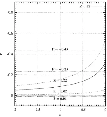
FIG. 2. The plot of P vs zlis shown by employing the ALEPH

ratio R⫽1.12⫾0.10. The experimental polarization P⫽

⫺0.23⫺0.20⫹0.24is also shown to indicate the allowed range of zl.

TABLE I. The values of the⌳bpolarization are predicted from the quark model, the parton model, the

modified quark model, and the modified parton model by employing the ALEPH and DELPHI experiments. The ALEPH and DELPHI experimental results are also shown for comparison.

PQM PPM PMQM PMPM PEXP R Experiment

⫺0.23⫺0.17⫹0.19 ⫺0.23⫺0.17⫹0.19 ⫺0.24⫺0.17⫹0.20 ⫺0.24⫺0.17⫹0.20 ⫺0.23⫺0.20⫹0.24 1.12⫾0.1 ALEPH

P⫽3共1⫺R兲 R⫺3zl

. 共86兲

Theoretically, the zlrange would be model dependent. By varying the value of t, we can easily change zl. This is because the suppressions from the contributions of intrinsic transverse momentum are modeled by parameter t. Consid-ering MQM and MPM and plotting the zl⫺t relation in Fig. 1, we can find that there is an upper bound for z_l as z_l⭐ ⫺0.05 with t⬃0.3, and a lower bound for zl as zl⭓⫺0.18 with t⬃2. The reason for existing the upper and lower bounds for zl is as follows. The fluctuations from the Bessel function in the differential decay rates would prevent the suppression of t from becoming large and small. In the end, there exist upper and lower bounds for zl. We also hope that t should be less than unity and close to zero to make the perturbative calculation reliable. Thus the z_lbound should be ⫺0.12⭐zl⭐⫺0.05 with the corresponding bound for t,0 ⭐t⭐0.3. Since, in the zl⫺t plot, the differences between the MPM and MQM are very small, we shall not distinguish tMQMand tMPM.

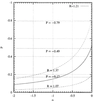
We now discuss the extraction of z_lfrom experiments. We first plot the behaviors of P with respect to zl for RALEPH

⫽1.12⫾0.10 共ALEPH兲 and RDELPHI_⫽1.21

⫺0.14

⫹0.16_{共DELPHI兲 in}

Figs. 2 and 3, respectively. By applying the experimental bounds for P, we can extract from Fig. 2 the z_l range of ⫺⬁⭐zl⭐⫺0.105 for ALEPH and from Fig. 3 the range of ⫺1.75⭐zl⭐⫺0.02 for DELPHI. We now discuss that the possible constraint over zl can be obtained from the OPAL experiment. The OPAL Collaboration employed a compari-son between the measured y 3⫽E_␯¯/E_l and the Monte Carlo simulated y₃MC to determine the polarization P⫽ ⫺0.56_⫺0.13⫹0.20_{(stat). Applying the OPAL P to the DELPHI and}

ALEPH experiments, we obtain ⫺0.6⭐z_l⭐⫺0.1 for DEL-PHI and ⫺0.55⭐zl⭐⫺0.105 for ALEPH. We summarize the above discussions for the determination of the zlin Table II. In the models we are considering, the lower bound for zl cannot be smaller than⫺0.12. We then assume that the range of zl can be obtained by combining the experimental and theoretical bounds. We thus have the zl range of⫺0.12⭐zl ⭐⫺0.105, and the corresponding t range of 0⭐t⭐0.05.

As a consistent check, we can write R in terms of P and zl as

R⫽3共1⫹Pzl兲

共3⫹P兲 . 共87兲

TABLE II. The bounds of zlare obtained from the ALEPH, DELPHI, and OPAL experiments, and from the theory. OPAL1 represents the combination of the OPAL and the ALEPH experiments, and OPAL2 the combination of the OPAL and the DELPHI experiments.

ALEPH DELPHI OPAL1 OPAL2 THEORY

⫺⬁⭐zl⭐⫺0.105 ⫺1.75⭐zl⭐⫺0.02 ⫺0.55⭐zl⭐⫺0.105 ⫺0.6⭐zl⭐⫺0.1 ⫺0.12⭐zl⭐⫺0.05

FIG. 3. The plot of P vs zlis shown by employing the DELPHI

ratio R⫽1.21_⫺0.14⫹0.16. The experimental polarization P⫽⫺0.49_⫺0.30⫹0.32is also shown to indicate the allowed range of zl.

FIG. 4. Plot of R vs P. The ALEPH and DELPHI Monte Carlo simulations共solid line兲 and the theoretical prediction 共band line兲 are shown.

By this equation, we can parametrize the Monte Carlo simu-lation ratios RMC( P)’s of ALEPH and DELPHI. We find that the value of zl⬃⫺0.075 can be used for both experiments in a good approximation within 5% –10%. In Fig. 4 we com-pare the R⫺P plots for zl⬃⫺0.075 and for ⫺0.12⭐zl⭐ ⫺0.105. The experimental bounds for ratio R can give con-straints over P. The combination of ALEPH and DELPHI experiments gives the range of P as ⫺0.79⭐P⭐⫺0.05, while our analysis results in⫺0.73⭐P⭐⫺0.05. The differ-ence between these two bounds of P can be reduced by in-cluding higher order corrections for the theory, such as the mass corrections, etc.

V. CONCLUSION

In this paper we have constructed four models based on the PQCD factorization formula for ⌳b→Xcl¯ . We used␯ these models to investigate the physics implied by the

ALEPH, OPAL, and DELPHI experiments. We found that these experiments can be understood from theoretical mod-els, the modified quark model and modified parton model. These two models contain intrinsic transverse momenta for partons, which are nonperturbative and parametrized by an exponential form with a parameter t. The parameter t relates to the variable zl⫽

具

Pl*( P⫽⫺1)

典

/

具

El*

典

with

具

Pl*( P⫽ ⫺1)

典

and

具

E_l*

典

the average momentum and energy of charge lepton in the rest frame of ⌳bbaryon. We found that the ratio R⫽y(P)/y(0) can be approximately expressed in terms of P and zl. Using experimental results, we then de-termined the ranges of zl and t.

ACKNOWLEDGMENTS

This work was supported in part by the National Science Council of R.O.C. under Grant No. NSC89-2811-M-009-0024.

关1兴 ALEPH Collaboration, D. Buskulic et al., Phys. Lett. B 365,

437共1996兲.

关2兴 OPAL Collaboration, G. Abbiendi et al., Phys. Lett. B 444,

539共1998兲.

关3兴 DELPHI Collaboration, Phys. Lett. B 474, 205 共2000兲. 关4兴 F.E. Close, J.G. Ko¨ner, R.J.N. Philips, and D.J. Summers, J.

Phys. G 8, 1719共1992兲.

关5兴 T. Mannel and G.A. Schular, Phys. Lett. B 279, 194 共1992兲. 关6兴 J.G. Ko¨rner, A. Pilaftsis, and M. Tung, Z. Phys. C 63, 575

共1994兲.

关7兴 J.H. Ku¨hn, A. Reiter, and P.M. Zerwas, Nucl. Phys. B272, 560 共1986兲.

关8兴 S. Jadach and Z. Was, Acta Phys. Pol. B 15, 1151 共1984兲. 关9兴 A.F. Falk and M.E. Peskin, Phys. Rev. D 49, 3320 共1994兲. 关10兴 J.G. Korner, Nucl. Phys. B 共Proc. Suppl.兲 50, 130 共1996兲. 关11兴 G. Bonvicini and L. Randall, Phys. Rev. Lett. 73, 392 共1994兲. 关12兴 H-n. Li and H.L. Yu, Phys. Rev. D 53, 4970 共1996兲.

关13兴 A.H. Mueller, Nucl. Phys. B250, 327 共1985兲.

关14兴 M. Beneke and V.I. Zakharov, Phys. Lett. B 312, 340 共1993兲. 关15兴 V.I. Zakharov, Nucl. Phys. B385, 452 共1992兲.

关16兴 G.P. Korchemsky and G. Sterman, Phys. Lett. B 340, 96 共1994兲.