STANDARDIZED CATCH PER UNIT EFFORT OF BIGEYE TUNA (THUNNUS OBESUS) FOR THE TAIWANESE LONGLINE FISHERY IN THE ATLANTIC OCEAN BY GENERAL ADDITIVE MODEL

(1)

SCRS/2007/063 Collect. Vol. Sci. Pap. ICCAT, 62(2): 372-396 (2008)

STANDARDIZED CATCH PER UNIT EFFORT OF BIGEYE TUNA (THUNNUS

OBESUS) FOR THE TAIWANESE LONGLINE FISHERY IN THE ATLANTIC

OCEAN BY GENERAL ADDITIVE MODEL

Chien-Chung Hsu1

SUMMARY

Abundance index of bigeye tuna (Thunnus obesus) in the Atlantic Ocean from Taiwanese longline fishery are presented for the period 1981-2006 by general additive model. The index (number caught per 1,000 hooks) was generated from numbers of bigeye tuna caught and reported in the logbooks submitted by commercial fishermen since 1981. Variables used in standardization are year, area, season, targets that are represented as quantiles of ratios of albacore and yellowfin tuna in total catches of these three species and their interactions. Thus, a step-wise regression procedure was used to select the set of systematic factors and interactions that significantly explained the observed variability, and deviance analysis was used to select the most appropriate factors in the standardization for the proportion positive observations and the deviance for the positive catch rates. Final selection of explanatory factors was conditioned to the significance of chi-square test and the relative percentages of deviance explained by adding the factor in evaluation and normally, factors that explained more than 5 were selected. Consequently, factors of year, area, target on albacore, target on yellowfin tuna and year-area interaction were used in both models. The results of abundance index were obtained from multiplying positive catch rate, which was generated from a general linear mixed model (GLMM) with delta-lognormal error structure, and proportion of positive catch sets, which was obtained by GLMM with binomial error structure. Then two data sets were applied and the result obtained from monthly aggregated data by vessels and by 5-degree square are more reasonable. Different results obtained by different regions were also presented in the report. However, since the quarter factor is not significant, the quarterly standardized catch-per- unit-effort for regions were not available.

RÉSUMÉ

Ce document présente l’indice d’abondance du thon obèse (Thunnus obesus) de la pêcherie palangrière du Taïpei chinois dans l’Océan Atlantique pour la période 1981-2006, réalisé par modèle additif généralisé. Cet indice (nombre capturé par 1.000 hameçons) a été généré d’après le nombre de thons obèses capturés et déclarés dans les livres de bord soumis par les pêcheurs commerciaux depuis 1981. Les variables utilisées dans la standardisation sont l’année, la saison, les cibles, qui sont présentées comme quantiles des ratios du germon et de l’albacore en prises totales de ces trois espèces et leurs interactions. Une procédure de régression pas à pas a donc été utilisée pour sélectionner le jeu de facteurs systématiques et les interactions qui expliquent largement la variabilité observée. Une analyse de déviance a été utilisée pour sélectionner les facteurs les plus appropriés dans la standardisation pour la proportion des observations positives et la déviance pour les taux de capture positifs. La sélection finale des facteurs explicatifs dépendait de l’importance du test du chi-deux et des pourcentages relatifs de déviance, expliqués en rajoutant le facteur dans l’évaluation ; les facteurs qui en expliquaient plus de cinq ont généralement été sélectionnés. On a donc utilisé, dans les deux modèles, les facteurs année, zone, ciblage du germon, ciblage de l’albacore, et l’interaction année-zone. Les résultats de l’indice d’abondance ont été obtenus en multipliant le taux de capture positif, qui a été généré d’après un modèle linéaire généralisé mixte (GLMM) avec une structure d’erreur delta-lognormale et une proportion d’opérations de pêche positives, obtenues par GLMM avec une structure d’erreur binomiale. Deux jeux de données ont alors été appliqués et le résultat obtenu des données regroupées par mois et par carrés de 5 degrés est plus raisonnable. Le présent rapport inclut aussi différents résultats obtenus par différentes régions. Toutefois, étant donné que le facteur trimestre n’est pas important, la capture par unité d’effort standardisée par trimestre pour ces régions n’était pas disponible.

1

(2)

RESUMEN

Se presentan los índices de abundancia de patudo (Thunnus obesus) en el océano Atlántico para la pesquería palangrera de Taipei Chino durante el periodo 1981-2006, mediante un modelo generalizado aditivo. Se obtuvo el índice (número capturado por 1.000 anzuelos) a partir del número de ejemplares de patudo capturados y comunicados en los cuadernos de pesca presentados por los pescadores comerciales desde 1981. Las variables utilizadas en la estandarización fueron año, zona, temporada, especie objetivo, representada como cuantiles de ratios de atún blanco y rabil en las capturas totales de estas tres especies, y sus interacciones. Por tanto, se utilizó un procedimiento de regresión gradual para seleccionar un conjunto de interacciones y factores sistemáticos que explicaban en gran medida la variabilidad observada. Se utilizó el análisis de devianza para seleccionar los factores más apropiados en la estandarización para la proporción de observaciones positivas y la devianza para las tasas de captura positivas. La selección final de factores explicativos estuvo condicionada por la importancia de la prueba de chi cuadrado y los porcentajes relativos de devianza que se explicaban al añadir el factor a la evaluación y se seleccionaron los factores que explicaban más de 5. Por consiguiente, los factores año, zona, estrategia de pesca dirigida al atún blanco, estrategia de pesca dirigida al rabil e interacción zona-año se utilizaron en ambos modelos. Los resultados del índice de abundancia se obtuvieron multiplicando la tasa de captura positiva, que se generó a partir de un modelo lineal mixto generalizado (GLMM) con una estructura de error delta-lognormal, y la proporción de lances de captura positivos, que se obtuvo mediante un GLMM con una estructura de error binomial. A continuación se aplicaron dos conjuntos de datos y los resultados obtenidos de los datos agregados mensualmente por buques y por cuadrículas de 5º fueron más razonables. En este documento se presentan también los diferentes resultados obtenidos para las diferentes regiones. Sin embargo, dado que el factor trimestre no es significativo, la captura por unidad de esfuerzo estandarizada trimestralmente no estaba disponible.

KEYWORDS

Bigeye tuna (Thunnus obesus), abundance index, GLMM, longline,

delta lognormal distribution, binomial distribution, deep longline fishing pattern, logbook

1. Introduction

Bigeye tuna (Thunnus obesus), is the most valuable and cosmopolitan scombridae, distributing in the tropical and temperate waters between 45°N and 45°S (Collette and Nauen, 1983). In the Atlantic Ocean, the species has been targeting by many fisheries including Taiwanese longline fishery mainly since 1990, although significant catches before 1989 were also reported previously (Hsu and Chen, 1996) as non-targeted. The annual production by all fleets in the entire Atlantic bigeye tuna stock has exceeded 100,000 tons since 1995, and Taiwanese catches have been limited to 16,500 tons since 1998.

The stock status was first evaluated in 1997 using only the standardized catch per unit effort of the Japanese longline fishery (Satoh et al. 2003). The results obtained indicated that the stock was fully exploited, especially the spawning stock biomass, which has declined since the early 1990s (Anon., 2003). The previous standardized catch per unit effort for Taiwanese series (Hsu, 1999; Hsu and Lee, 2003) showed a great variation from year to year and stratified sub-area, because of the non homogeneous distribution of logbook recovery in the early 1990s in space and time.

Information on the relative abundance is always necessary to tuna stock assessment models. Catch per unit effort (CPUE) from commercial fisheries has been used to derive indices of relative abundance or to estimate fishing effort for many world fisheries (Gulland, 1956; Robson, 1996; Large, 1992; Stefansson, 1996; Griffin et al., 1997; Goni et al., 1999). However, the use of catch rates in constructing abundance indices requires standardization to take into account changes in the ability to catch fish, fleet composition, and to adjust catch rate estimates for other factors that may affect the catch rates such as year, month, boat type, or abundance of other target species in the catch (Hilborn and Walters, 1992). The generalized additive modeling (GAM) technique with general linear mixed models (GLMM) and delta log-normal distribution for the positive catch rate and binomial distribution for the proportion of positive bigeye tuna catch, respectively, is used because (1) GLMM extends from generalized linear model (GLM) which allows identification of the factors that influence catch rates as well as computation of standardized catch rates, represented by the year effect factor. The factor levels in GLMM are considered as randomly selected from a population of all possible factor levels and the model does

(3)

not allow only one source of randomness from error structure; and (2) the delta log-normal distribution avoids problems with contagion by zero data and treats zero and nonzero data separately (Lo et al., 1992).

This study is an attempt to address the above two issues in standardizing catch rates of bigeye tuna: (1) to identify factors that have significant effects on catch rates of this species; and (2) to produce a time series of standardized catch rate estimates that can be used for stock assessments.

2. Materials and methods 2.1 Data used

Two data sets were used in the present analysis. First, the 5x5 squared catch-effort data for bigeye tuna were compiled from logbooks of Taiwanese longline fishery in the Atlantic Ocean for the period 1981 to 2006. And second, the aggregated data set from pooling daily records of logbooks, i.e. the logbook data were pooled vessel by vessel for monthly 5x5 square data. The second dataset was very similar to TASKII without raising to TASK I. For convenience, the new dataset was called “TASKII” hereinafter.

There were many changes either in the fishery or in the statistical system during the previous two decades for Taiwanese longline fishery. Those changes may provide different information on the interpretation of standardized abundance index, which include: first, the fishery has been starting to target bigeye tuna since 1990 (about 12,000 t). The catch was found notable from 1994 (about 20,000 t) with historical high level appeared in 1996 (about 22,000 t), but has then declined significantly in 1998 due the catch limit of 16,500 t annually set specifically to the fishery, and an abrupt quota reduction to 4,500 t in 2006. Those quotas had been shared to both bigeye vessels (mainly) and albacore vessels (partially), so some of the albacore vessels may have reported a significant bigeye tuna catch which the information may be involved in the analysis of the bigeye tuna abundance index.

Second, the responsible organization for logbook compilation has changed in 1995 on the logbook data from 1994 onwards, from Institute of Oceanography, National Taiwan University (IONTU) to Oversea Fisheries Development Council (OFDC). Logbook of 1991-1993 has been revised after that time in the consideration to increase very low logbook coverage (originally less than 5%). But even with such revision, the coverage of 1991-93 is still low comparing to the current coverage level of 40-60%.

2.2 Stratification of sub-area

Sub-area defined for bigeye tuna (Figure 1) used in this study is assigned as in the “Bigeye tuna work plan: year 2002,” which is stratified the bigeye tuna fishing area in the Atlantic Ocean into 12 strata. Each area is assumed to approximately have homogeneous species density with the investigation of nominal catch per unit effort by 5x5 squared area catch records and those stratified sub-areas were used in the following standardized process as the area factor. Also a larger sub-area was stratified as in Figure 1 for trying to develop a new abundance index for MULTIFAN-CL analysis.

2.3 Model used for standardization

Relative indices of abundance for bigeye tuna were generated by Generalized Linear Mixed Model (GLMM) approach assuming a delta-lognormal error distribution for the positive catch rates. The delta model fits separately the proportion of positive sets assuming a binomial error distribution and the mean catch rate of sets if at least one fish was caught assuming a lognormal error distribution. The standardized index is the product of these two independent model-estimated components. The estimated proportion of successful sets per stratum is assumed to be the result of

r

positive sets of a total

n

number of sets, and each one is an independent Bernoulli-type realization. The estimated proportion is a linear function of fixed effects and interactions. The logit function was used as a link between linear factor components and binomial errors. For positive observations, which were defined as at least one bigeye tuna caught, the estimated CPUE rate was assumed to follow a lognormal error distribution (lnCPUE-nominal) of a linear function of fixed factors and random effect interactions, particularly when the

year

effect was within the interaction.

A step-wise regression procedure was used to determine the set of systematic factors and interactions that significantly explained the observed variability. Then the Chi-square (

χ

2) distribution was used to test the difference of deviance between two consecutive models, that is, this statistic was used to test significance of an additional factor in the model and the number of additional parameters associated with the added factor minus

(4)

one corresponds to the number of degree of freedom in the

χ

2 test (McCullagh and Nelder, 1989). Deviance analysis tables are presented for both data series, each table includes the deviance for the proportion of positive observations (i.e. positive sets/total sets), and the deviance for the positive catch rates. Final selection of explanatory factors was conditional to (1) the relative percentage of deviance explained by adding the factor in evaluation (normally factors that explained more than 5 to 10 % were selected); (2) significance of the

χ

2 test; and (3) the type III test of significance within the final specified model.

Once a set of fixed factors was specified, possible interactions were evaluated, in particular interactions between the

year

effect and other factors. Relative indices for the delta model formulation were calculated as the product of the year effect least square means (LSMeans) from the binomial and the lognormal model components. The LSMeans estimates use a weighted factor of the proportional observed margins in the input data to account for the un-balanced characteristics of the data. All models using the stepwise approach were fitted with the SAS GEBNOD procedure, whereas the final model was run with the SAS GLIMMIX and MIXED procedures (SAS Inst. Inc.). The detail of GLMM statistical algorithm of standardization for catch per unit effort was described in Lo et al. (1992).. For the model, the average positive catch rate was for instance; a logarithmic transformation of observed positive catch rate is represented by factors of year, sub-area, targets and their interaction as:

(

_y_,_a_,_f

)

=

₀

+

_y

+

_a

+

_f

+

_y_,_a

+

_f_,_a

+

_y_,_f

+

z

log

μ

α

(1) And the probability that at least catch one fish is a log-normal density:

(

2

)

, , , , , ,a ft

~

ya f

,

a f y

LogNorm

u

z

σ

(2) Further, the proportion of positive catch can be expressed as:

w

f y a f a y f a y f a y f a y

₌

₊

⎟

⎠

⎞

⎜

⎝

⎛

−

0 , , , , , , ,

1 log

β

ρ

(3)

with a binomial density:

(

ya f ya f

)

f a

y

Bin

n

w

_, _,

~

_, _,

,

ρ

_, _, (4) The computation was pursued by SAS version 8.2.

3. Results

3.1 Nominal catch per unit effort

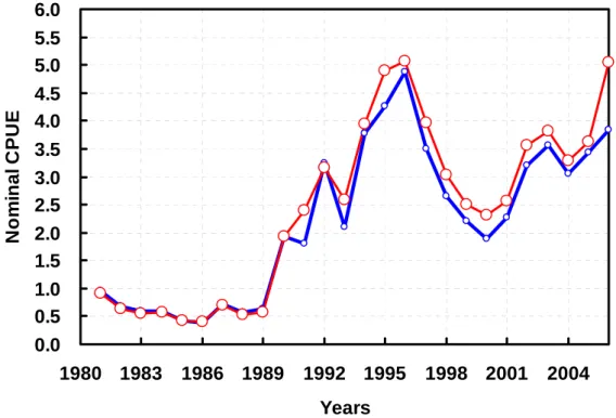
Nominal catch per unit effort series (number of fish per 1,000 hooks) of bigeye tuna caught by the Taiwanese longline fleets was estimated by the total number of catch divided the total number of hooks summing up from daily logbooks and from the TASKII data sets, and is illustrated in Figure 2. The nominal catch per unit depicts that a flat trend till 1989, an increasing trend from 1990 to 1996, then a sharp decline to 2000, and a slight increasing trend since then with a little drop in 2004. The nominal series obtained from TASKII dataset was coincident with the series obtained from daily logbooks. Both series almost have the same value before 1990; however, the TASKII series has significantly lower values than the logbook series.

3.2 Standardization of catch per unit effort

3.2.1 Logbook databases

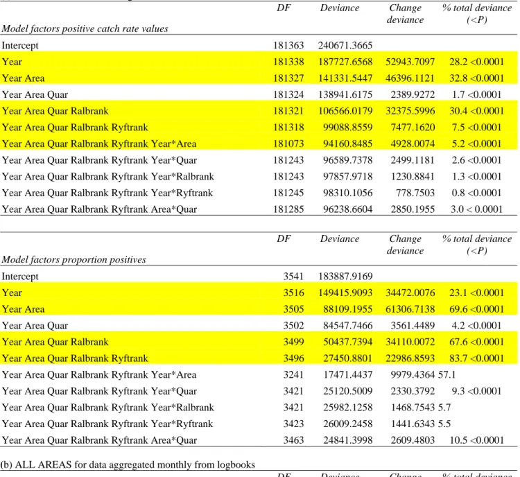
As shown in Table 1, the analysis of deviance explains that factors of year, sub-area, catch of albacore, catch of yellowfin tuna and year-sub-area interaction are significant for Chi-square test (

p

<0.0001) and percentage of deviance on standardizing positive catch rate; and factors of year, sub-area, catch of albacore and yellowfin tuna are significant for Chi-square test (

p

<0.0001) and percentage of deviance for proportion positive sets. Then,

(5)

these mentioned factors were selected in GLMM model to standardize catch per unit effort of bigeye tuna caught by Taiwanese longline fishery in the Atlantic from 1981 to 2006. The quarter factor was not significant for both of positive catch rate and positive proportion analyses.

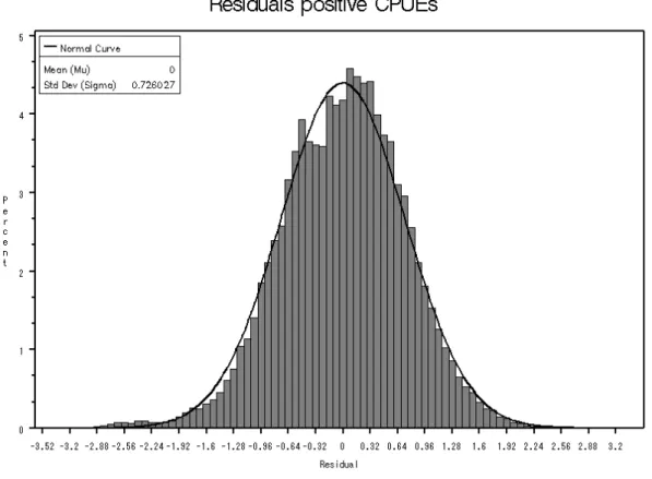
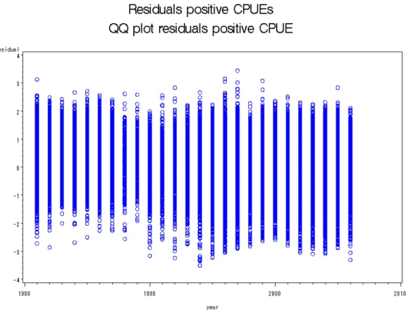
Thus, for logbook dataset the standardized positive catch rate, standardized proportion of positive catch and the standardized catch per unit effort were shown in Figures 3, 4 and 5, respectively. For validating the standardization, a normal residual frequency distribution, QQ plot to detect the relation between residuals and normal quantiles, residual distribution with year and residuals of the binomial distribution for the proportion of positive sets by years was illustrated in Figures 6, 7 and 8, respectively. All the error structures were investigated and followed the lognormal distribution for standardizing positive catch rate and following binomial distribution for the proportion of positive catch. Therefore, the standardization of catch per unit effort of bigeye tuna for Taiwanese longline fishery using daily logbook data and applying to GAM is validated.

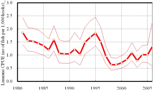
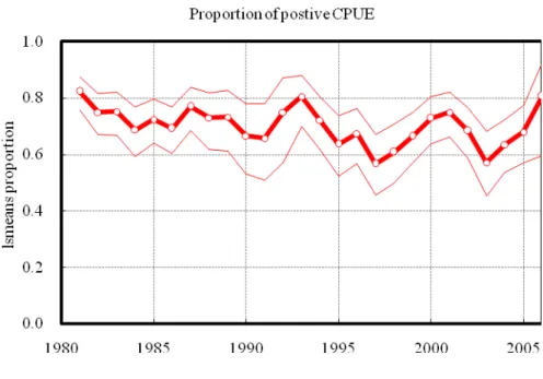
The standardized positive catch rate shows decreasing trend from 1981 to1992, abrupt increase to 1994, then declined continuously to 2001, then increased to about 1990’ level in 2001 and maintained fluctuated in this level (Figure 3). The proportion of positive catch was maintained in 0.5-0.6 level before 1995, and dropped to below 0.4 in 1998, then increased to the 0.5-06 level then after (Figure 4). And the integrate standardization of abundance index (Figure 5) shows decreasing trend from 1981 to 1992, and increases to the highest level for the series in 1995, then declines to the lowest level in 1998 and 1999, and increased again to the level of 1990’s.

3.2.2 Task II dataset

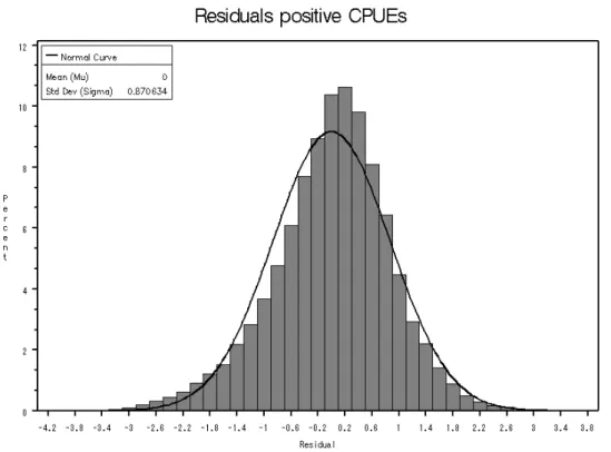
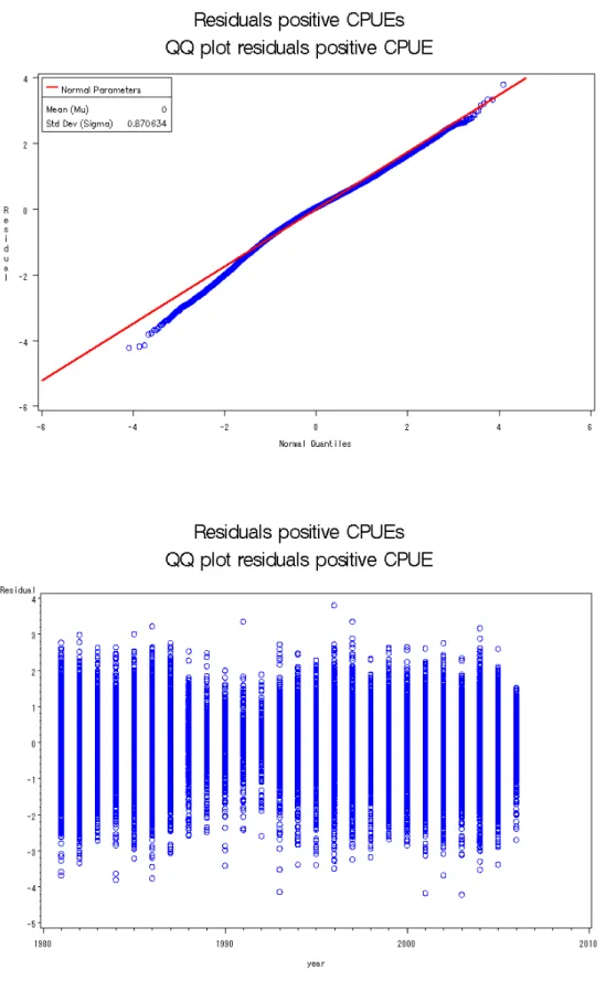
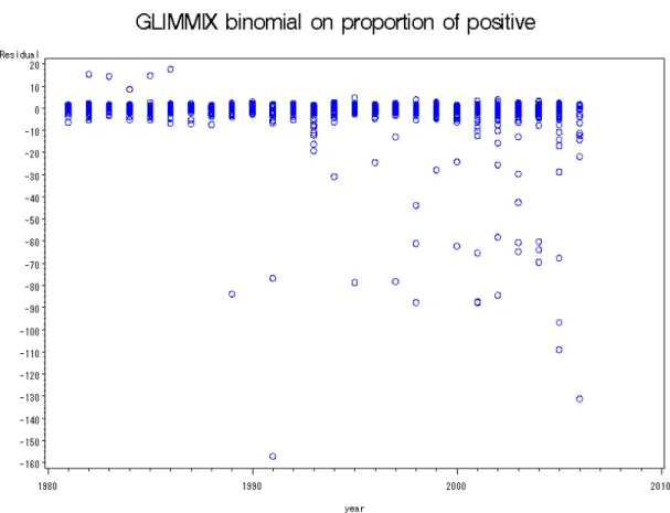
For Task II dataset the standardized positive catch rate, standardized proportion of positive catch and the standardized catch per unit effort were shown in Figures 9, 10 and 11, respectively. For validating the standardization, a normal residual frequency distribution, QQ plot to detect the relation between residuals and normal quantiles, residual distribution with year and residuals of the binomial distribution for the proportion of positive sets by years was illustrated in Figures 12, 13 and 14, respectively. All the error structures were investigated and followed the lognormal distribution for standardizing positive catch rate and following binomial distribution for the proportion of positive catch. Therefore, the standardization of catch per unit effort of bigeye tuna for Taiwanese longline fishery using aggregated daily logbook data (Task II) and applying to GAM is validated.

The standardized positive catch rate shows decreasing trend from 1981 to1988 with great fluctuation, kept flat to 1991 and slightly decreased in 1992, increased to 1994, then declined slightly to 1996 and continuously and abruptly to 1998, then increased slightly in a historical low level to 2001 and slightly increased and maintained fluctuated in this level (Figure 9) then after. The proportion of positive catch was maintained in 0.6-0.8 level for the entire series (Figure 10). And the integrate standardization of abundance index (Figure 11) shows slight fluctuation with decreasing trend from 1981 to 1992 with a incident peak in 1987, and increases to 1994, then declines to the lowest level in 1998, and increased again to 2002, decreases in 2003 and increases further to 2006 with the level of mid-1990s.

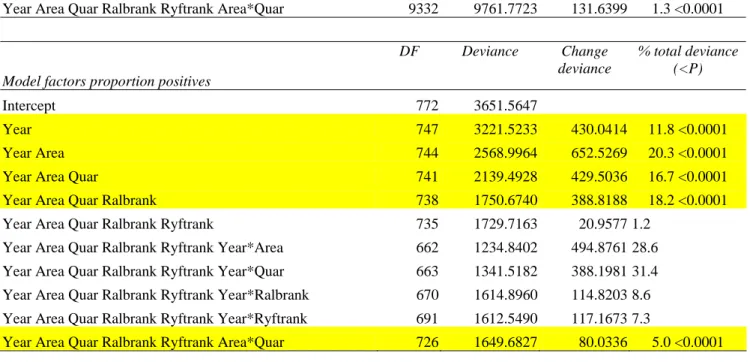
3.2.3 Regional standardized catch per unit effort using Task II dataset

The region stratification was mapped in Figure 2. Since the factors examined by step-wise regression and deviance analysis showed different factors significant in different regions (Table 1b), a different factors was used in standardization for different regions. The validation using examination of error structure assumption was presented. For region I, QQ plot to detect the relation between residuals and normal quantiles, a normal residual frequency distribution, residual distribution with year was illustrated in Figures 15, 16 and 17, respectively. And residuals of the binomial distribution for the proportion of positive sets by years were not available, since none of the examined was significant (Table 1b).

For region II, QQ plot to detect the relation between residuals and normal quantiles, a normal residual frequency distribution, and residual distribution with year and residuals of the binomial distribution for the proportion of positive sets by years was illustrated in Figures 18, 19 and 20, respectively.

For region III, QQ plot to detect the relation between residuals and normal quantiles, a normal residual frequency distribution, and residual distribution with year and residuals of the binomial distribution for the proportion of positive sets by years was illustrated in Figures 21, 22 and 23, respectively.

(6)

Consequently, the time series of abundance index for bigeye tuna estimated by entire Atlantic with logbook and TASKII data sets and by regions by TASKII data set shows in Figure 24. Standardized catch per unit effort of region II shows much fluctuated and of region III shows decreasing trend from 2005.

4. Discussion

There were several trials (e.g., Hsu 1999; Hsu and Liu 2000; 2001; Hsu and Lee 2002) to standardize bigeye tuna abundance index using Taiwanese longline catch and effort data from Atlantic Ocean. However, those trials need to be verified for their fitness to the fishery, and the results are uncertain due to the possible effects from the changes that have been mentioned in the Material and Methods section, in particular, the change of target species in early 1990s (Hsu and Lin 1996), the change of logbook compilation system and the setting of catch limit since 1998. Further investigations will be needed for deriving more reliable abundance index.

Further, information of a number of hooks per basket (between two floats, NHPB) was added in the logbooks for all Taiwanese distant waters longline vessels from 1995 onward, however, the percentages of returned logbooks with NHPB information were still very low. So the information seemed not useful in standardization. Lin (1998), Yeh et al. (2001) and Lee et al. (2004) have attempted to use a learning data set, which is built from the returned logbooks with NHPB, to separate the daily set in the returned logbooks without NHPB into either deep or regular longline pattern. The separation result was said about 67.7% being classified correctly in according to Lee-Nishida. method (Lee et al. 2004). However, if we do this so by Lin method (Lin 1998) and by Yeh method (Yeh et al. 2001), which almost look like Lee-Nishda method (Lee et al. 2004), the result was still not satisfactory (Hsu and Lee 2002). Consequently, the separation of fishing patterns seems not helpful on the standardization of bigeye tuna for Taiwanese longline fishery in the Atlantic. As the result, a general additive model (GAM) was used in the present study to avoid separating fishing patterns. Thus, the proportion of positive catch and positive catch rate were applied to daily sets collected from logbooks of Taiwanese longline fishery and their aggregated by vessel and by 5-degree block (TASKII data set) for GAM. And GAM may solve the problem of fishing patterns, particularly for the TASKII data set.

However, due to unbalance allocation of collection of logbooks, which were from deep longline vessels or regular longline vessels, the estimation of proportion positive catch (a probability to catch at least one bigeye tuna) may be biased. The obvious condition was occurred as in 2006, which almost all return logbooks are from deep longline vessels because followed ICCAT recommendation (05-01).

During the analysis, some daily sets were collected from small-scaled longline fishery. And the analysis was incorporated with those small-scaled longline fishery data without expelling those data out, because it is not possible to separate those data out at this moment. But this needs to be done in future study.

5. References

ANON. 1999. Bigeye tuna – 1998 Detailed Report. International Commission for the Conservation of Atlantic Tunas, Collect. Vol. Sci. Pap. ICCAT, 49(3): 1-93.

ANON. 2004. Bigeye tuna – 2003 Detailed Report. International Commission for the Conservation of Atlantic Tunas, Collect. Vol. Sci. Pap. ICCAT, 56(2): 282-352.

BERRY, D.A. 1987. Logarithmic transformations in ANOVA. Biometrics. 43: 439-456.

COLLETTE, B.B. and C.E. Nauen. 1983. FAO Species Catalogue. Vol. 2. Scombrids of the world. FAO

Fisheries Synopsis No. 125 (2): 1-137.

FOX, D.S. and R.M. Starr. 1996. Comparison of commercial fishery and research catch data. Can. J. Aquat. Sci. 53: 2681-2694.

GONI, R., F. Alvarez, and S. Adlerstein. 1999. Application of generalized linear modeling to catch rate analysis of western Mediterranean fisheries: the Castellon trawl fleet as a case study. Fish. Res. 42: 291-302.

GRIFFIN, W.L., A.K. Shah, and J.M. Nance. 1997. Estimation of standardized effort in the heterogeneous Gulf of Mexico shrimp fleet. Mar. Fish. Rev. 59(3): 23-33.

GULLAND, J.A. 1956. On the fishing effort in English demersal fisheries. Fish. Invest., London Ser. 2(20): 1-41.

(7)

HILBORN, R., and C.J. Walters. 1992. Quantitative Fisheries Stock Assessment, Choice, Dynamics and

Uncertainty. Chapman & Hall, London.

HSU, C.C. 1999. Standardized abundance index of Taiwanese longline fishery for bigeye tuna in the Atlantic. Collect. Vol. Sci. Pap. ICCAT, 49(3): 459-465.

HSU, C.C. and Y.C. Chen. 1996. Recent Taiwanese longline fisheries in the Atlantic. Collect. Vol. Sci. Pap. ICCAT, 45(2): 62-67.

HSU, C.C. and H.H. Lee. 2003. General linear mixed model analysis for standardization of Taiwanese longline CPUE for bigeye tuna in the Atlantic Ocean. Collect. Vol. Sci. Pap. ICCAT, 55(5): 1892-1915.

HSU, C.C. and M.C. Lin. 1996. The recent catch estimation procedure of Taiwanese longline fishery. Collect. Vol. Sci. Pap. ICCAT, 43:171-178.

HSU, C.C. and H.C. Liu. 2000. The updated catch per unit effort of bigeye tuna for Taiwanese longline fishery in the Atlantic. Collect. Vol. Sci. Pap. ICCAT, 51:635-650.

HSU, C.C. and H.C. Liu. 2001. Verificatin of bigeye tuna length and catch data consistency for Taiwanese longline fishery in the Atlantic. Collect. Vol. Sci. Pap. ICCAT, 54(1):172-190.

ICCAT. 1997. Report for Biennial Period, 1996-1997, Part I (1996), Vol. 1 and 2. Madrid, Spain.

LARGE, P.A. 1992. Use of a multiplicative model to estimate relative abundance from commercial CPUE data.

ICES J. Mar. Sci. 49: 253-261.

LEE, Y.C., T. Nishida and M. Mohri. 2004. Separation of the Taiwanese regular and deep tuna longliners in the Indian Ocean using bigeye tuna catch rations. (Manuscript).

LIN, C.J. 1998. The relationship between Taiwanese longline fishing patterns and catch compositions in the Indian Ocean. M.S. Thesis, Institute of Oceanography, National Taiwan University, Taipei. 57pp.

LO, N.C., L.D. Jacobson, and J.L. Squire. 1992. Indices of relative abundance from fish spotter data based on delta-lognormal models. Can. J. Fish. Aquat. Sci. 49: 2515-2526.

MA, C.T. and C.C. Hsu. 1997. Standardization of CPUE for yellowfin tuna caught by Taiwanese longline fishery in the Atlantic. Collect. Vol. Sci. Pap. ICCAT, 46(4): 197-204.

MCCULLAGH, P. and J.A. Nelder. 1989. Generalized Linear Models 2nd edition. Chapman & Hall.

SATOH, K., H. Okamoto and N. Miyabe. 2003. Abundance indices of Atlantic bigeye caught by the Japanese longline fishery and related information updated as of 2002. Collect. Vol. Sci. Pap. ICCAT, 55(5): 2004-2027.

STEFANSSON, G. 1996. Analysis of groundfish survey abundance data: combining the GLM and delta approaches. ICES J. Mar. Sci. 53: 577-588.

YEH, Y. M., C.C. Hsu, H.H. Lee and H.C. Liu. 2001. A new method for categorizing Taiwanese longline catch and effort data to improve abundance index standardization. (Manuscript).

(8)

Table 1. Deviance analysis table of explanatory variables in the delta lognormal model for bigeye tuna catch rates (in number per 1,000 hooks) for Taiwanese longline fishery from 1981 to 2004. Percentages of total deviance refer to the deviance explained by the full model, and p values indicate the 5% Chi-square probability between consecutive models.

(a) ALL AREAS for data of logbooks

Model factors positive catch rate values

DF Deviance Change deviance % total deviance (<P) Intercept 181363 240671.3665 Year 181338 187727.6568 52943.7097 28.2 <0.0001 Year Area 181327 141331.5447 46396.1121 32.8 <0.0001

Year Area Quar 181324 138941.6175 2389.9272 1.7 <0.0001

Year Area Quar Ralbrank 181321 106566.0179 32375.5996 30.4 <0.0001 Year Area Quar Ralbrank Ryftrank 181318 99088.8559 7477.1620 7.5 <0.0001 Year Area Quar Ralbrank Ryftrank Year*Area 181073 94160.8485 4928.0074 5.2 <0.0001 Year Area Quar Ralbrank Ryftrank Year*Quar 181243 96589.7378 2499.1181 2.6 <0.0001 Year Area Quar Ralbrank Ryftrank Year*Ralbrank 181243 97857.9718 1230.8841 1.3 <0.0001 Year Area Quar Ralbrank Ryftrank Year*Ryftrank 181245 98310.1056 778.7503 0.8 <0.0001 Year Area Quar Ralbrank Ryftrank Area*Quar 181285 96238.6604 2850.1955 3.0 < 0.0001

Model factors proportion positives

Year Area Quar 3502 84547.7466 3561.4489 4.2 <0.0001

Year Area Quar Ralbrank 3499 50437.7394 34110.0072 67.6 <0.0001

Year Area Quar Ralbrank Ryftrank 3496 27450.8801 22986.8593 83.7 <0.0001 Year Area Quar Ralbrank Ryftrank Year*Area 3241 17471.4437 9979.4364 57.1

Year Area Quar Ralbrank Ryftrank Year*Quar 3421 25120.5009 2330.3792 9.3 <0.0001 Year Area Quar Ralbrank Ryftrank Year*Ralbrank 3421 25982.1258 1468.7543 5.7

Year Area Quar Ralbrank Ryftrank Year*Ryftrank 3423 26009.2458 1441.6343 5.5

Year Area Quar Ralbrank Ryftrank Area*Quar 3463 24841.3998 2609.4803 10.5 <0.0001

(b) ALL AREAS for data aggregated monthly from logbooks

DF Deviance Change deviance % total deviance (<P) Intercept 29363 71809.2684 Year 29338 55762.5459 16046.7225 22.3 <0.0001 Year Area 29327 37677.7116 18084.8343 32.4<0.0001

Year Area Quar 29324 37245.8906 431.8210 1.1 <0.0001

Year Area Quar Ralbrank Ryftrank 29318 24054.4142 1388.5771 5.5 <0.0001 Year Area Quar Ralbrank Ryftrank Year*Area 29072 22044.1227 2010.2915 8.4 <0.0001 Year Area Quar Ralbrank Ryftrank Year*Quar 29243 23063.9174 990.4968 4.5 <0.0001 Year Area Quar Ralbrank Ryftrank Year*Ralbrank 29244 23583.5659 470.8483 2.0 <0.0001

(9)

Year Area Quar Ralbrank Ryftrank Year*Ryftrank 29250 23795.2109 259.2033 1.1 <0.0001 Year Area Quar Ralbrank Ryftrank Area*Quar 29285 22973.5003 1080.9139 4.5 <0.0001

DF Deviance Change deviance % total deviance (<P) Intercept 2369 14878.8903 Year 2344 13494.1874 1384.7029 9.3 <0.0001 Year Area 2333 8347.3994 5146.7880 38.1<0.0001

Year Area Quar 2330 8006.1635 341.2359 4.1 <0.0001

Year Area Quar Ralbrank Ryftrank Year*Quar 2249 4357.8093 409.9672 13.6<0.0001 Year Area Quar Ralbrank Ryftrank Year*Ralbrank 2250 4467.7254 300.0511 6.9

Year Area Quar Ralbrank Ryftrank Year*Ryftrank 2255 4485.2486 282.5279 6.3

Region 1

Year Area Quar 2864 2907.9125 10.4504 0.4 0.0157

Year Area Quar Ralbrank Ryftrank 2858 2733.7303 5.2882 0.2 0.01336 Year Area Quar Ralbrank Ryftrank Year*Area 2839 2635.6065 98.1238 3.6 <0.0001 Year Area Quar Ralbrank Ryftrank Year*Quar 2806 2585.3672 148.3631 5.6 <0.0001 Year Area Quar Ralbrank Ryftrank Year*Ralbrank 2837 2625.6401 108.0902 4.2 <0.0001 Year Area Quar Ralbrank Ryftrank Year*Ryftrank 2851 2687.6236 46.1067 1.8 <0.0001 Year Area Quar Ralbrank Ryftrank Area*Quar 2855 2650.1563 83.5740 3.1 <0.0001

DF Deviance Change deviance % total deviance (<P) Intercept 177 592.4833 Year 152 286.1474 306.3359 51.7 Year Area 151 282.0012 4.1462 1.4

Year Area Quar 148 275.3409 6.6603 2.4

Year Area Quar Ralbrank 145 267.9128 7.4281 2.7

Year Area Quar Ralbrank Ryftrank 142 259.7279 8.1849 3.1

Year Area Quar Ralbrank Ryftrank Year*Area 123 212.3077 47.4202 18.3

Year Area Quar Ralbrank Ryftrank Year*Quar 80 120.4929 139.2350 65.6 Year Area Quar Ralbrank Ryftrank Year*Ralbrank 118 210.3203 49.4076 41.0 Year Area Quar Ralbrank Ryftrank Year*Ryftrank 133 232.0885 27.6394 13.1

(10)

Year Area Quar Ralbrank Ryftrank Area*Quar 139 256.7889 2.9390 1.3

Region 2

DF Deviance Change deviance % total deviance Intercept 17094 32518.3483 Year 17069 21275.6327 11242.7156 34.6 <0.0001 Year Area 17064 18053.1495 3222.4832 15.1 <0.0001

Year Area Quar 17061 17613.1283 440.0212 2.4 <0.0001

Year Area Quar Ralbrank Ryftrank 17055 10010.7448 1156.9230 10.4<0.0001 Year Area Quar Ralbrank Ryftrank Year*Area 16946 9504.1208 506.6240 5.1 <0.0001 Year Area Quar Ralbrank Ryftrank Year*Quar 16984 9555.0781 455.6667 4.8 <0.0001 Year Area Quar Ralbrank Ryftrank Year*Ralbrank 16990 9655.4809 355.2639 3.7 <0.0001 Year Area Quar Ralbrank Ryftrank Year*Ryftrank 16990 9842.0716 168.6732 1.7 <0.0001 Year Area Quar Ralbrank Ryftrank Area*Quar 17040 9844.9520 165.7928 1.7 <0.0001

Year Area Quar 1385 4787.6613 105.5698 2.2 <0.0001

Year Area Quar Ralbrank Ryftrank Year*Quar 1304 1425.1868 306.6896 24.0 Year Area Quar Ralbrank Ryftrank Year*Ralbrank 1313 1470.0782 261.7982 18.4 Year Area Quar Ralbrank Ryftrank Year*Ryftrank 1313 1533.7799 198.0965 13.5

Region 3

Year Area Quar 9347 12994.9489 551.5835 4.1 <0.0001

Year Area Quar Ralbrank Ryftrank 9341 9893.4122 217.6709 2.2 <0.0001 Year Area Quar Ralbrank Ryftrank Year*Area 9269 9161.0803 732.3319 7.4 <0.0001 Year Area Quar Ralbrank Ryftrank Year*Quar 9270 9403.1266 490.2856 5.4 <0.0001 Year Area Quar Ralbrank Ryftrank Year*Ralbrank 9277 9635.5172 257.8950 2.7 <0.0001 Year Area Quar Ralbrank Ryftrank Year*Ryftrank 9302 9759.6057 133.8065 1.4 <0.0001

(11)

Year Area Quar 741 2139.4928 429.5036 16.7 <0.0001

Year Area Quar Ralbrank Ryftrank 735 1729.7163 20.9577 1.2

Year Area Quar Ralbrank Ryftrank Year*Area 662 1234.8402 494.8761 28.6 Year Area Quar Ralbrank Ryftrank Year*Quar 663 1341.5182 388.1981 31.4 Year Area Quar Ralbrank Ryftrank Year*Ralbrank 670 1614.8960 114.8203 8.6 Year Area Quar Ralbrank Ryftrank Year*Ryftrank 691 1612.5490 117.1673 7.3

Figure 1. Area stratification of Atlantic for standardizing bigeye tuna catch per unit effort.

I

II

(12)

0.0

0.5

1.0

1.5

2.0

2.5

3.0

3.5

4.0

4.5

5.0

5.5

6.0 1980

1983

1986

1989

1992

1995

1998

2001

2004

Years

No

m

in

a

l CP

UE

Figure 2. Nominal CPUE of bigeye tuna for Taiwanese longline fishery in the Atlantic from 1981 to 2006, estimated from logbooks (red curve) and monthly aggregated data (blue curve) for positive catch.

Figure 3. Standardized CPUE of bigeye tuna for Taiwanese longline fishery in the Atlantic from 1981 to 2006, estimated from logbooks for positive catch.

(13)

Figure 4. Observed probability of positive sets to catch bigeye tuna for Taiwanese longline fishery in the Atlantic, estimated from daily records of logbooks from 1981 to 2006.

Figure 5. Standardized CPUE of bigeye tuna for Taiwanese longline fishery in the Atlantic from 1981 to 2006, estimated from daily logbooks.

(14)

Figure 6. Residual frequency distribution of positive catch rate sets with delta lognormal errors for bigeye tuna caught by Taiwanese longline fleets in the Atlantic from 1981 to 2006.

Figure 7. The Q-Q plot for the residuals of using general linear mixed model with delta log-normal error structure to standardize observed positive catch rate of bigeye tuna caught by Taiwanese longline fishery in the Atlantic from 1981 to 2006.

(15)

Figure 8. Diagnostic plot: Chi-square residuals of the residuals of the lognormal assumed error distribution for the positive sets (upper), and binomial assumed error distribution for the proportion of positive sets of bigeye tuna (lower).

(16)

Figure 9. Standardized CPUE of bigeye tuna for Taiwanese longline fishery in the Atlantic from 1981 to 2006, estimated from monthly aggregated data of logbooks for positive catch.

Figure 10. Observed probability of positive sets for Taiwanese longline fishery in the Atlantic, estimated from monthly aggregated data of daily records of logbooks from 1981 to 2006.

(17)

Figure 11. Standardized CPUE of bigeye tuna for Taiwanese longline fishery in the Atlantic from 1981 to 2006, estimated from monthly aggregated data of logbooks.

Figure 12. Residual frequency distribution of positive catch rate sets with delta lognormal errors for bigeye tuna caught by Taiwanese longline fleets in the Atlantic from 1981 to 2006.

(18)

Figure 13. The Q-Q plot for the residuals of using general linear mixed model with delta log-normal error structure to standardize observed positive catch rate of bigeye tuna caught by Taiwanese longline fishery in the Atlantic from 1981 to 2006.

(19)

Figure 14. Diagnostic plot: Chi-square residuals of the binomial assumed error distribution for the proportion of positive sets of bigeye tuna (upper), and residuals of the lognormal assumed error distribution for the positive sets (lower).

Figure 15. The Q-Q plot for the residuals of using general linear mixed model with delta log-normal error structure to standardize observed positive catch rate of bigeye tuna caught by Taiwanese longline fishery in the Atlantic from 1981 to 2006 for region I.

(20)

Figure 16. Residual frequency distribution of positive catch rate sets with delta lognormal errors for bigeye tuna caught by Taiwanese longline fleets in the Atlantic from 1981 to 2006 for region I.

Figure 17. Diagnostic plot: Chi-square residuals of the residuals of the lognormal assumed error distribution for the positive sets (upper), and binomial assumed error distribution for the proportion of positive sets of bigeye tuna (lower) for Region I..

(21)

Figure 18. The Q-Q plot for the residuals of using general linear mixed model with delta log-normal error structure to standardize observed positive catch rate of bigeye tuna caught by Taiwanese longline fishery in the Atlantic from 1981 to 2006 for region II.

Figure 19. Residual frequency distribution of positive catch rate sets with delta lognormal errors for bigeye tuna caught by Taiwanese longline fleets in the Atlantic from 1981 to 2006 for region II.

(22)

Figure 20. Diagnostic plot: Chi-square residuals of the residuals of the lognormal assumed error distribution for the positive sets (upper), and binomial assumed error distribution for the proportion of positive sets of bigeye tuna (lower) for Region II.

(23)

Figure 21. The Q-Q plot for the residuals of using general linear mixed model with delta log-normal error structure to standardize observed positive catch rate of bigeye tuna caught by Taiwanese longline fishery in the Atlantic from 1981 to 2006 for region III.

Figure 22. Residual frequency distribution of positive catch rate sets with delta lognormal errors for bigeye tuna caught by Taiwanese longline fleets in the Atlantic from 1981 to 2006 for region III.

(24)

Figure 23. Diagnostic plot: Chi-square residuals of the residuals of the lognormal assumed error distribution for the positive sets (upper), and binomial assumed error distribution for the proportion of positive sets of bigeye tuna (lower) for Region III.

(25)

Figure 24. Time series of standardized abundance indices of bigeye tuna by Taiwanese longline fishery, estimated by integrating the results from the binomial and lognormal error models for Taiwanese longline fishery from 1981 to 2006 for the entire Atlantic by different data sets and by regions.