在巨量資料上的平行多核心線性分類算法

全文

(1)國立臺灣大學電機資訊學院資訊工程學系學士班學生論文 Department of Computer Science and Information Engineering College of Electrical Engineering and Computer Science. National Taiwan University Bachelor Degree Thesis. 在巨量資料上的平行多核心線性分類算法 Parallel Large-scale Linear Classification in Multi-core Environments. 江韋霖 Wei-Lin Chiang. 指導教授：林智仁博士 Advisor: Chih-Jen Lin, Ph.D.. 中華民國 106 年 4 月 April, 2017.

(2) 國立臺灣大學學士班學生論文. 口試委員會審定書在巨量資料上的平行多核心線性分類算法 Parallel Large-scale Linear Classification in Multi-core Environments 本論文係江韋霖君（學號 B02902056）在國立臺灣大學資訊工程學系完成之學士班學生論文，於民國 106 年 4 月 28 日承下列考試委員審查通過及口試及格，特此證明. 口試委員：（簽名）（指導教授）. 系主任.

(3) 摘要. 在機器學習領域裡，線性分類模型如線性支持向量機、邏輯回歸，是一類被廣泛使用的分類算法，然而在處理大規模資料的問題時，模型的訓練仍需耗費大量時間完成，因此本文旨在利用多核心處理器的優勢來加速巨量資料上的線性模型的訓練，首先我們考慮以矩陣運算為瓶頸的優化算法做加速，並特別針對牛頓法深入研究，結果顯示在合適的實作下，牛頓法能獲得非常優異的加速效果。此外我們也針對另一類重要算法—對偶座標下降法做分析，並提出一套架構使得平行加速可以有效的應用至此，且保證其理論收斂性，透過實驗多方比較，我們展示了該算法在多核心環境下優異的效率及穩定性。. 關鍵字：大規模線性分類、牛頓法、對偶座標下降法、平行運算. ii.

(4) Abstract. Linear classification such as linear SVM and logistic regression is one of the most used machine learning methods. However, the training process for large-scale data can still be slow. In this work, we focus on utilizing the power of multi-core CPUs for parallelizing linear classification optimization methods. First, we consider methods that can take the advantage of parallel matrix operations and particularly investigate a Newton method for large-scale logistic regression. Results indicate that under suitable settings excellent speedup can be achieved. Then we analyze parallel dual-based methods, which are another important methods to train large-scale linear classifiers. We propose a theoretically sound framework for parallelizing dual methods and demonstrate through experiments that the new framework is robust and efficient in a multi-core environment.. Keywords: large-scale linear classification, Newton methods, dual coordinate descent, parallel computation. iii.

(5) Contents 口試委員會審定書 . . . . . . . . . . . . . . . . . . . . . . . . . . . . . . . . . .. i. 摘要 . . . . . . . . . . . . . . . . . . . . . . . . . . . . . . . . . . . . . . . . . .. ii. Abstract . . . . . . . . . . . . . . . . . . . . . . . . . . . . . . . . . . . . . . . .. iii. Contents . . . . . . . . . . . . . . . . . . . . . . . . . . . . . . . . . . . . . . . .. iv. List of Figures . . . . . . . . . . . . . . . . . . . . . . . . . . . . . . . . . . . . .. vii. List of Tables . . . . . . . . . . . . . . . . . . . . . . . . . . . . . . . . . . . . . viii 1. Introduction . . . . . . . . . . . . . . . . . . . . . . . . . . . . . . . . . . . .. 1. 2. Fast Matrix-vector Multiplications in Newton Method . . . . . . . . . . . . . .. 4. 2.1. 2.2. Sparse Matrix-vector Multiplications in Newton Methods for Logistic Regression . . . . . . . . . . . . . . . . . . . . . . . . . . . . . . . . . . .. 5. 2.1.1. Baseline: Single-core Implementation in LIBLINEAR . . . . . . .. 6. 2.1.2. Parallel Matrix-vector Multiplication by OpenMP . . . . . . . . .. 7. 2.1.3. Combining Matrix-vector Operations . . . . . . . . . . . . . . .. 8. 2.1.4. Sparse Matrix-vector Multiplications by Intel MKL . . . . . . . .. 9. 2.1.5. Sparse Matrix-vector Multiplications with the Recursive Sparse Blocks Format . . . . . . . . . . . . . . . . . . . . . . . . . . .. 10. Experiments . . . . . . . . . . . . . . . . . . . . . . . . . . . . . . . . .. 12. 2.2.1. Data Sets and Experimental Settings . . . . . . . . . . . . . . . .. 12. 2.2.2. Running Time of Sparse Matrix-vector Multiplications in Newton Methods. . . . . . . . . . . . . . . . . . . . . . . . . . . . . . .. iv. 13.

(6) 3. 2.2.3. Comparison on Matrix-vector Multiplications . . . . . . . . . . .. 14. 2.2.4. Detailed Analysis on Implementations using OpenMP . . . . . .. 15. 2.2.5. Results on Newton Methods for Solving (2.1) . . . . . . . . . . .. 16. 2.2.6. Summary of Experiments . . . . . . . . . . . . . . . . . . . . .. 17. Parallel Dual Coordinate Descent Method . . . . . . . . . . . . . . . . . . . .. 18. 3.1. Dual Coordinate Descent and Difficulties of Its Parallelization . . . . . .. 19. 3.1.1. Linear Classification and Dual CD Methods . . . . . . . . . . . .. 19. 3.1.2. Difficulties in Parallelizing Dual CD . . . . . . . . . . . . . . . .. 22. A Framework for Parallel Dual CD . . . . . . . . . . . . . . . . . . . . .. 26. 3.2.1. Our Idea for Parallelization . . . . . . . . . . . . . . . . . . . . .. 27. 3.2.2. A General Framework for Parallel Dual CD . . . . . . . . . . . .. 30. 3.2.3. Relation with Decomposition Methods for Kernel SVM . . . . .. 32. Theoretical Properties and Implementation Issues . . . . . . . . . . . . .. 35. 3.3.1. Shrinking . . . . . . . . . . . . . . . . . . . . . . . . . . . . . .. 36. 3.3.2. ¯ . . . . . . . . . . . . . . . . . . . . . . . . . . . The Size of |B|. 36. 3.3.3. Adaptive Condition in Choosing B . . . . . . . . . . . . . . . .. 37. Experiments . . . . . . . . . . . . . . . . . . . . . . . . . . . . . . . . .. 38. 3.4.1. Analysis of Algorithm 4 . . . . . . . . . . . . . . . . . . . . . .. 39. 3.4.2. Comparison of Algorithms 4 and 6 . . . . . . . . . . . . . . . . .. 41. 3.4.3. Comparison of Parallel Dual CD Methods . . . . . . . . . . . . .. 42. Discussion and Conclusions . . . . . . . . . . . . . . . . . . . . . . . .. 44. 3.2. 3.3. 3.4. 3.5. 3.5.1. Multi-CPU Environments and the Comparison with Parallel Newton Methods . . . . . . . . . . . . . . . . . . . . . . . . . . . .. 44. 3.5.2. Using ∇P f (α) or α − P [α − ∇f (α)] . . . . . . . . . . . . . .. 45. 3.5.3. Conclusions . . . . . . . . . . . . . . . . . . . . . . . . . . . . .. 46. v.

(7) 4. Conclusions . . . . . . . . . . . . . . . . . . . . . . . . . . . . . . . . . . . .. 47. A Appendix . . . . . . . . . . . . . . . . . . . . . . . . . . . . . . . . . . . . .. 48. A.1 Matrix-vector Multiplications in Newton Methods for Logistic Regression. 48. A.1.1 Newton and Truncated Newton Methods . . . . . . . . . . . . .. 48. A.1.2 Line Search Procedure . . . . . . . . . . . . . . . . . . . . . . .. 50. A.1.3 Trust Region Methods . . . . . . . . . . . . . . . . . . . . . . .. 51. A.1.4 Computational Cost . . . . . . . . . . . . . . . . . . . . . . . .. 52. A.2 Detailed Analysis on Implementation using OpenMP . . . . . . . . . . .. 52. A.2.1 Relations with Asynchronous Coordinate Descent Methods . . . .. 54. Bibliography . . . . . . . . . . . . . . . . . . . . . . . . . . . . . . . . . . . . .. 58. vi.

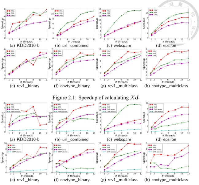
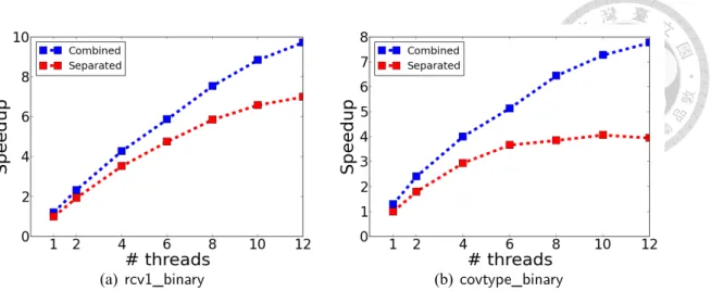
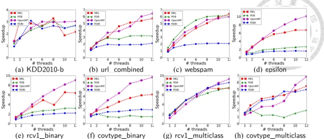
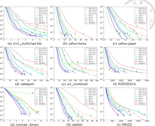
(8) List of Figures 2.1. Speedup of calculating Xd . . . . . . . . . . . . . . . . . . . . . . . . .. 10. 2.2. Speedup of calculating X T u, where u = DXd. . . . . . . . . . . . . . .. 10. 2.3. Speedup of calculating Xd and X T u separately and together . . . . . . .. 13. 2.4. Speedup of the Newton method for training logistic regression . . . . . .. 14. 3.1. A comparison of two multi-core dual CD methods: asynchronous CD and Algorithm 4, and one single-core implementation: LIBLINEAR. We present the relation between training time in seconds (x-axis) and the relative difference to the optimal objective value (y-axis, log-scaled). The l1. 3.2. loss is used. . . . . . . . . . . . . . . . . . . . . . . . . . . . . . . . . .. 40. The same comparison as in Figure 3.1 except that the l2 loss is used. . . .. 41. vii.

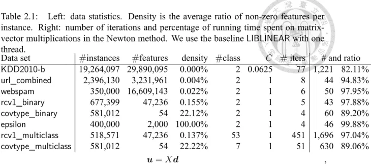
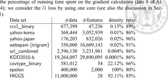
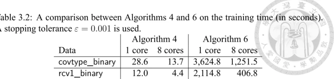
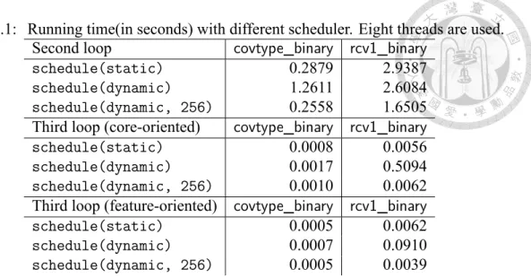
(9) List of Tables 2.1. Left: data statistics. Density is the average ratio of non-zero features per instance. Right: number of iterations and percentage of running time spent on matrix-vector multiplications in the Newton method. We use the baseline LIBLINEAR with one thread. . . . . . . . . . . . . . . . . . . . . . .. 3.1. 7. Data statistics: Density is the average ratio of non-zero features per instance. Ratio is the percentage of running time spent on the gradient calculation (line 8 of Algorithm 4); we consider the l1 loss by using one core (see also the discussion in Section 3.4.1). . . . . . . . . . . . . . . . . .. 3.2. 39. A comparison between Algorithms 4 and 6 on the training time (in seconds). A stopping tolerance ε = 0.001 is used. . . . . . . . . . . . . . . .. 42. A.1 Running time(in seconds) with different scheduler. Eight threads are used.. 54. viii.

(10) 1. Introduction Linear classification such as linear SVM and logistic regression is one of the most. widely used machine learning methods, but training large-scale data remains a time-consuming process. To reduce the training time, many parallel classification algorithms have been proposed for shared-memory or distributed environments. In this work, we target at shared-memory systems because nowadays a typical server possesses enough memory to store reasonably large data and multi-core CPUs are widely used. A high performance code in a multi-core shared-memory system should possess the following properties. 1. Synchronization between threads should be avoided. Then one thread does not need to wait for results of another. 2. The communication between CPUs or cores should be minimized. Although the memory is shared, some recent systems (e.g., Intel Xeon) have the NUMA (nonuniform memory access) architecture, so each CPU has its own cache. A processor can access data in its own local cache faster than those in another. 3. The access time of moving data from lower-level memory (e.g., main memory) to upper-level memory (e.g., cache) should be minimized. Indeed the first and the second issues are also encountered by parallel algorithms in distributed environments, although the second issue becomes more serious because of the expensive communication between nodes. In contrast, the third issue on memory access. 1.

(11) is sometimes the major concern in shared-memory systems. To be focused here, we restrict our discussion to methods that are suitable for multi-core shared-memory systems. Therefore, some methods that are mainly applicable in distributed environments are out of our interests. Existing optimization methods for linear classification can be roughly categorized to the following two types: 1. Low-order optimization methods such as stochastic gradient (SG) or coordinate descent (CD) methods. By using only the gradient information, this type of methods runs many cheap iterations. 2. High-order optimization methods such as quasi Newton or Newton methods. By using, for example, second-order information, each iteration is expensive but fewer iterations are needed to approach the final solution. These methods, useful in different circumstances, have been parallelized in some past works, for example, [2, 15, 17, 23, 37, 39]. Some target at distributed environments, but some others are for shared-memory systems. These algorithms are often designed by extending existing machine learning algorithms to parallel settings. For example, stochastic gradient (SG) and coordinate descent (CD) methods are efficient methods for data classification [1, 14], but they process one data instance at a time. The algorithm is inherently sequential because the next iteration relies on the result of the current one. For parallelization, researchers have proposed modifications so that each node or thread independently conducts SG or CD iterations on a subset of data. To avoid synchronization between threads, the machine learning model may be updated by one thread without considering the progress in others [15, 31]. An issue of asynchronous updates is that convergence must be proved and analyzed following the modification from the original setting. Because asynchronous settings may have convergence issues, we consider methods in a serial setting and speed up every single iteration. The first approach is to check if 2.

(12) parallel linear algebra modules can be applied to some machine learning algorithms. For example, if Newton methods are used to train logistic regression for large-scale document data, the data matrix is sparse and sparse matrix-vector multiplications are the main computational bottleneck [20, 26]. If we can apply fast implementations of matrix operations, then machine learning algorithms can be parallelized without any modification. In Chapter 2, we investigate various implementations of fast matrix-vector multiplications when they are applied to the Newton method for large-scale linear classification. Experiments show that we can achieve significant speedup on a typical server. In particular, a carefully designed implementation using OpenMP [6] is simple and efficient. The second approach is to discuss parallel approaches on low-order optimization methods which do not have expensive matrix operations in each iteration. For low-order methods, we are particularly interested in the CD method to solve the dual optimization problem as it has become one of the most efficient methods for large-scale linear classification after the recent introduction [14]. Further, in contrast to primal-based methods (e.g., Newton or primal CD) that often require the differentiability of loss functions, a dual-based method can handle some non-differentiable losses such as the l1 hinge loss (i.e., linear SVM). In Chapter 3, we detailedly discuss existing approaches for parallel dual CD methods, and demonstrate why they may be inefficient or unstable under some situations. Then we propose a framework that can effectively take the advantage of multi-core computations and theoretical properties of convergence are also provided. Finally, through experiments and comparisons we show that our proposed method is robust and efficient. This bachelor thesis is based on the two published works [5, 24]. Based on results in this thesis, we develop a multi-core extension of LIBLINEAR including several parallelization methods. It is available at http://www.csie.ntu.edu.tw/~cjlin/libsvmtools/ multicore-liblinear. According to users’ feedback, this multi-core extension has been used for improving the training speed of some real-world applications. 3.

(13) 2. Fast Matrix-vector Multiplications in Newton Method Although our goal is to employ fast sparse matrix operations for machine learning. algorithms, we must admit that unlike dense matrix operations, the development has not been as successful. It is known that sparse matrix operations may be memory bound [3, 4, 28]. That is, CPU waits for data being read from lower-level to upper-level memory. The same situation has appeared for dense matrix operations, but optimized implementations have been well studied by the numerical analysis community. The result is the successful optimized BLAS in the past several decades. BLAS (Basic Linear Algebra Subprograms) is a standard set of functions defined for vector and dense matrix operations [7, 8, 22]. By carefully designing the algorithm to reduce cache/memory accesses, an optimized matrixmatrix or matrix-vector multiplication can be much faster than a naive implementation. However, because of the complication on the quantity and positions of non-zero values, such huge success has not applied to sparse matrices. Fortunately, intensive research has been conducted recently so some tools for fast sparse matrix-vector multiplications are available (e.g., [3, 28]). With the recent progress on the fast implementation of matrix-vector multiplications, it is time to investigate if applying them to some machine learning algorithms can reduce the running time. In compared with the many existing works on parallel machine learning, an. 4.

(14) obvious advantage is that no new algorithms must be developed. The existing convergence still holds and the same model is obtained as before. In this chapter, we focus on Newton methods for large-scale logistic regression. In Section 2.1, we point out that the computational bottleneck of Newton methods for logistic regression is on matrix-vector multiplications. We then investigate several state-of-theart strategies for sparse matrix-vector multiplications. Through experiments are in Section 2.2 to illustrate how we achieve good speedup. Some materials including the connection to [15] can be found in Appendix.. 2.1. Sparse Matrix-vector Multiplications in Newton Methods for Logistic Regression. Logistic regression is widely used for classification. Given training instances {(yi , xi )}li=1 with label yi = ±1 and feature vector xi ∈ Rn , logistic regression solves the following convex optimization problem to obtain a model vector w.. min w. ∑l 1 T f (w) ≡ wT w + C i=1 log(1 + e−yi w xi ), 2. (2.1). where C > 0 is the regularization parameter, l is the number of instances, n is the number of features. Many optimization methods have been proposed for training large-scale logistic regression. Among them, Newton methods are reliable approaches [20, 21, 26]. Assume the data matrix is [. ]T. X = x1 , . . . , xl. 5. ∈ Rl×n ..

(15) It is known that at each Newton iteration the main computational task is on a sequence of Hessian-vector products.. ∇2 f (w)d = (I + CX T DX)d,. (2.2). where ∇2 f (w) is the Hessian, I is the identity matrix, D is a diagonal matrix associated with the current w, and d is an intermediate vector. The detailed derivations are left in Appendix. Our focus in this work is thus on how to speedup the calculation of (2.2). From (2.2), the Hessian-vector multiplication involves. Xd,. D(Xd),. X T (DXd). The second step takes only O(l) because D is diagonal. Subsequently we investigate efficient methods for the first and the third steps.. 2.1.1. Baseline: Single-core Implementation in LIBLINEAR. By the nature of data classification, currently LIBLINEAR implements an instancebased storage so that non-zero entries in each xi can be easily accessed. Specifically, xi is an array of nodes and each node contains feature index and value: xi →. index1. index2. index4. index4. value1. value2. value4. value4. .... Note that we modify a figure in [27] here. This type of row-based storage is common for sparse matrices, where the most used one is the CSR (Compressed Sparse Row) format [35]. However, we note that the CSR format separately saves feature indices (i.e., column indices of X) and feature values in two arrays, so it is slightly different from the above implementation in LIBLINEAR. For the matrix-vector multiplication, 6.

(16) Table 2.1: Left: data statistics. Density is the average ratio of non-zero features per instance. Right: number of iterations and percentage of running time spent on matrixvector multiplications in the Newton method. We use the baseline LIBLINEAR with one thread. #instances #features # and ratio Data set density #class C # iters KDD2010-b 19,264,097 29,890,095 0.000% 2 0.0625 77 1,221 82.11% 2,396,130 3,231,961 0.004% 44 94.83% url_combined 2 1 8 webspam 350,000 16,609,143 0.022% 2 1 6 50 97.95% rcv1_binary 677,399 47,236 0.155% 2 1 5 43 97.88% covtype_binary 2 1 4 581,012 54 22.12% 60 89.20% 2,000 100.00% 1 epsilon 400,000 2 4 46 99.88% rcv1_multiclass 518,571 47,236 0.137% 53 1 451 1,696 97.04% 581,012 54 22.22% 630 89.06% covtype_multiclass 7 1 51 u = Xd , LIBLINEAR implements the following simple loop 1: for i = 1, . . . , l do. ui = xTi d. 2:. For the other matrix-vector multiplication ¯ = X T u, where u = DXd, u we can use the following loop 1: for i = 1, . . . , l do. ¯ ←u ¯ + ui xi u. 2:. ¯ = u1 x1 + · · · + ul xl . By this setting there is no need to calculate and store X T . because u. 2.1.2. Parallel Matrix-vector Multiplication by OpenMP. We aim at parallelizing the two loops in Section 2.1.1 by OpenMP [6], which is simple and common in shared-memory systems. For the first loop, because xTi d, ∀i are independent, we can easily parallelize it by 1: for i = 1, . . . , l in parallel do 2:. ui = xTi d It is known [3] that parallelizing the second loop is more difficult because threads 7.

(17) ¯ at the same time. A common solution is that, after ui (xi )s is calculated, cannot update u we update u¯s by an atomic operation that avoids other threads to write u¯s at the same time. Specifically, we have the following loop. 1: for i = 1, . . . , l in parallel do. for (xi )s ̸= 0 do. 2:. atomic: u¯s ← u¯s + ui (xi )s. 3:. This loop of calculating X T u by atomic operations is related to the recent asynchronous parallel coordinate descent methods for linear classification [15]. In Appendix, we discuss the relationship between our results and theirs. An alternative approach to calculate X T u without using atomic operations is to store ˆp = u. ∑. {ui xi | i run by thread p}. during the computation, and sum up these vectors in the end. This approach essentially simulates a reduction operation in parallel computation: each thread has a local copy of the results and these local copies are combined for the final result. Currently, OpenMP supports reduction for scalars rather than arrays for C/C++, so we must handle these local arrays by ourself. The extra storage is in general not a concern because if the data set is ˆ p , ∀p is not extremely sparse and the number of cores is not super high, then the size of u ˆ p , ∀p should relatively smaller than the data size. Similarly, the extra cost for summing u be minor, but we will show in Section 2.2.4 that appropriate settings are needed to ensure fast computation.. 2.1.3. Combining Matrix-vector Operations. Although in Section 2.1.2 we have two separate loops for Xd and X T (DXd), from. X T DXd =. ∑l i=1. 8. xi Dii xTi d,. (2.3).

(18) the two loops can be combined together. For example, if we take the approach of temˆ p , p = 1, . . . , P , where P is the total number of threads, then the porarily storing arrays u implementation becomes 1: for i = 1, . . . , l in parallel do 2:. ui = Dii xTi d. 3:. ˆp = u ˆ p + ui xi , where p is the thread ID u. Although the number of operations is the same, because of accessing x1 , . . . , xl only once rather than twice, this approach should be better than the two-loop setting in Section 2.1.2. However, currently this is not what implemented in LIBLINEAR. Regarding the implementation efforts and the availability, this approach can be easily implemented by OpenMP. However, for existing sparse matrix packages such as those we will discuss in Sections 2.1.4 and 2.1.5, currently they do not support X T Xd type of operations. Therefore, the two operations involving X and X T must be separately conducted. The formulation (2.3) is the foundation of distributed Newton methods in [27, 39], where data are split to disjoint blocks, each node considers its local block and calculates ˆp = u. ∑. {ui xi | i run by node p}. ˆ p up to get u ¯ . In a shared-memory system, a core and then a reduce operation sums all u does not have its local subset, but we show in Section 2.2.5 that letting each thread work on a block of instances is very essential to achieve better speedup.. 2.1.4. Sparse Matrix-vector Multiplications by Intel MKL. Intel Math Kernel Library (MKL) is a commercial library including optimized routines for linear algebra. It supports fast matrix-vector multiplications for different sparse formats. We consider the commonly used CSR format to store X. Note that MKL provides. 9.

(19) (a) KDD2010-b. (b) url_combined. (c) webspam. (d) epsilon. (e) rcv1_binary. (f) covtype_binary. (g) rcv1_multiclass. (h) covtype_multiclass. Figure 2.1: Speedup of calculating Xd. (a) KDD2010-b. (b) url_combined. (c) webspam. (d) epsilon. (e) rcv1_binary. (f) covtype_binary. (g) rcv1_multiclass. (h) covtype_multiclass. Figure 2.2: Speedup of calculating X T u, where u = DXd. subroutines for X T u with X as the input.. 2.1.5. Sparse Matrix-vector Multiplications with the Recursive Sparse Blocks Format. Following the concept of splitting the matrix to blocks for dense BLAS implementations, [28] applies a similar idea for multiplications.  For example,   sparse matrix-vector  X1,1 d1 + X1,2 d2  X1,1 X1,2      .  ⇒ u = Xd =  X=     X2,1 d1 + X2,2 d2 X2,1 X2,2 This setting possesses the following advantages. First, X1,1 d1 and X1,2 d2 are indepen-. dent to each other, so two threads can be used to compute them simultaneously. Second, Each sub-matrix is smaller, so it occupies a smaller part of the higher-level memory (e.g., 10.

(20) cache). Then the chance that u and d are thrown out of cache during the computation becomes smaller. We illustrate this point by an extreme example. Suppose the cache is not enough to store xi and d together. In calculating xT1 d, we sequentially load elements in x1 and d to cache. By the time the inner product is done, d’s first several entries have been removed from the cache. Then for xT2 d, the vector d must be loaded again. In contrast, by using blocks, each time only part of xi and d are used, so the above situation may not occur. In any program, if data are accessed from a lower-level memory frequently, then CPUs must wait until they are available. While the concept of using blocks is the same as that for dense matrices, the design as well as the implementation for sparse matrices are more sophisticated. Recently, RSB (Recursive Sparse Blocks) format [30] has been proposed as an effective format for fast sparse matrix-vector multiplications. It recursively partitions a matrix in quadrants. In the end a tree structure with sub-matrices in the leaves is generated. The recursive partition terminates according to some conditions on the sub-matrix (e.g., number of non-zeros). The following figure shows an example of an 8 × 8 matrix in the RSB format.. An important concern for using the RSB format is the cost of initial construction, where details are in [29]. Practically, it is observed in [28] that when single thread is used for initial construction as well as matrix-vector multiplication, the construction cost is about 20 to 30 multiplications. This cost is not negligible, but for Newton methods which need quite a few multiplications, we will check in Section 2.2 if using RSB is cost-effective. Like MKL, the package librsb that we will use includes X T u subroutines by taking X as the input. We do not compare with another block-based approach CSB [3] because [28] has shown that RSB is often competitive with CSB.. 11.

(21) 2.2. Experiments. We compare various implementations of sparse matrix-vector multiplications when they are used in a Newton method.. 2.2.1. Data Sets and Experimental Settings. We carefully choose data sets to cover different density and different relationships between numbers of instances and features. All data sets listed in Table 2.1 are available at the LIBSVM data set page. Note that we use the tri-gram version of webspam in our experiments. Besides two-class data sets, we consider several multi-class problems. In LIBLINEAR, a K-class problem is decomposed to K two-class problems by the one-versus-the-rest strategy. Because each two-class problem treats one class as positive and the rest as negative, all the K problems share the same x1 , . . . , xl . Their matrix-vector multiplications involve the same X and X T . We are interested in such cases because approaches like RSB need the initial construction only once. We choose C = 1 as the regularization parameter in (2.1). An exception is C = 0.0625 for KDD2010-b for shorter training time. Our code is based on LIBLINEAR [9], which implements a trust region Newton method [26]. We compare the following approaches to conduct matrix-vector multiplications in the Newton method. • Baseline: The one-core implementation in LIBLINEAR (Section 2.1.1) serves as the baseline in our investigation of the speedup. We use version 1.96. • OpenMP: We employ OpenMP to parallelize the loops for matrix-vector multiplications. The scheduling we used is schedule(dynamic,256), where details will be discussed in Section 2.2.4. For X T u we have two settings OpenMP-atomic and OpenMP-array.. 12.

(22) (a) rcv1_binary. (b) covtype_binary. Figure 2.3: Speedup of calculating Xd and X T u separately and together The first one considers atomic operations, while the second stores results of each thread to an array; see Section 2.1.2. • MKL: We use Intel MKL version 11.2; see Section 2.1.4. • RSB: the approach described in Section 2.1.5 by using the recursive sparse block format. We use version 1.2.0 of the package librsb at http://librsb.sourceforge.net. Experiments are conducted on machines with 12 cores of Intel Xeon E5-2620 CPUs which has 32K L1-cache, 256K L2-cache and 15360K shared L3-cache. Because past comparisons (e.g., [28]) involving MKL often use the Intel icc compiler, we use it for all our programs with the option -O3 -xAVX -fPIC -openmp. Our experiment uses 1, 2, 4, 6, 8, 10, 12 threads because the machine we used has up to 12 cores.. 2.2.2. Running Time of Sparse Matrix-vector Multiplications in Newton Methods. Although past works have pointed out the importance of sparse matrix-vector multiplications in Newton methods for data classification, no numerical results have been reported to show their cost in the entire optimization procedure. In Table 2.1, we show the percentage of running time spent on matrix-vector multiplications. Clearly matrix-vector. 13.

(23) (a) KDD2010-b. (b) url_combined. (c) webspam. (d) epsilon. (e) rcv1_binary. (f) covtype_binary. (g) rcv1_multiclass. (h) covtype_multiclass. Figure 2.4: Speedup of the Newton method for training logistic regression multiplications are the computational bottleneck because for almost all problems, more than 90% of the running time is spent on them. Therefore, it is very essential to parallelize the sparse matrix-vector multiplications in a Newton method.. 2.2.3. Comparison on Matrix-vector Multiplications. Although past works from numerical analysis and parallel processing communities have compared different strategies for matrix-vector multiplications, they did not use matrices from machine learning problems. It is interesting to see if our results are consistent with theirs. We present the result of. speedup =. running time of LIBLINEAR running time of the compared approach. versus the number of threads. Note that the speedup may be bigger than the number of threads because of the storage and algorithmic differences from the baseline. The speedup for Xd and X T (DXd) may be different, so we separately present results in Figures 2.1 and 2.2. Results indicate that all approaches give excellent speedup for calculating Xd. For some problems, the speedup is so good that it is much higher than the number of threads.. 14.

(24) For example, using eight threads, RSB achieves speedup higher than 12. This result is possible because while the baseline uses a row-based storage, RSB applies a block storage for better data locality. Between RSB and MKL there is no clear winner. This observation is slightly different from [28], which shows that RSB is better than MKL. One reason might be that [28] experimented with matrices close to squared ones, but ours here are not. Although OpenMP’s implementation is the simplest, it enjoys good speedup. For X T u with u = DXd, in general the speedup becomes worse than that for Xd. For a few cases the difference is significant (e.g., RSB for covtype_binary). Like the situation for Xd, there is no clear winner between RSB and MKL. For the two OpenMP implementations for X T u, OpenMP-atomic completely fails to gain any speedup. Although we pointed out in Section 2.1.2 the possible delay of using atomic operations, such poor results are not what we expected. In contrast, OpenMP-array gives good speedup and is sometimes even better than RSB or MKL. From this experiment we see that even for the simple implementation by OpenMP, a careful design of algorithms for the loops can make significant differences.. 2.2.4. Detailed Analysis on Implementations using OpenMP. Following the dramatic difference between OpenMP-atomic and OpenMP-array for X T (DXd), we learned that having a suitable implementation by OpenMP is non-trivial. Therefore, we devote this subsection to thoroughly investigate some implementation issues. First we discuss the two implementations of computing Xd and X T (DXd) separately (Section 2.1.2) and together by (Section 2.1.3). Note that OpenMP-array is used here because of the much better speedup than OpenMP-atomic. Figure 2.3 presents the speedup of the two settings. The approach of using (2.3) in Section 2.1.3 is better because data. 15.

(25) instances x1 , . . . , xl are accessed once rather than twice. We already see improvement in the one-core situation, so (2.3) is what should have been implemented in LIBLINEAR. Interestingly, the gap between the two approaches widens as the number of threads increases. An explanation is that the doubled number of data accesses cause problems when more threads are accessing data at the same time. Based on this experiment, from now on when we refer to the OpenMP implementation, we mean (2.3) with the OpenMP-array setting. Next we investigate the implementation of OpenMP-array. We show in Appendix that without suitable settings (in particular, the scheduling of OpenMP loops), speedup can be poor.. 2.2.5. Results on Newton Methods for Solving (2.1). Figure 2.4 presents the speedup of the Newton method using various implementations for matrix-vector multiplications. Note that we consider end-to-end running time after excluding the initial data loading and the final model writing. Therefore, the construction time for transforming the row-based format to RSB is now included. This transformation does not occur for other approaches. For RSB, results in Section 2.2.3 indicate that its speedup for Xd is excellent, but is poor for X T u. Therefore, we consider a variant RSBt that generates and stores the RSB format of X T in the beginning. Although more memory is used, we hope that the speedup for X T u can be as good as that for Xd. Results in Figure 2.4 show that OpenMP (the version presented in Section 2.1.3) is the best for almost all cases, while MKL comes the second. RSB is worse than MKL mainly because of the following reasons. First, from Figure 2.2, RSB is mostly worse than MKL for X T u. Second, the construction time is not entirely negligible. Regarding. 16.

(26) RSBt, although we see better speedup for X T u, where details are not shown because of space limitation, the overall speed is worse than RSB for two-class problems. The reason is because that the construction time is doubled. However, for multi-class problems, RSBt may become better than RSB. Because several binary problems on the same data instances are solved, the construction time for the RSB format of X T has less impact on the total training time. The speedup for KDD2010-b is worse than others because it has the lowest percentage of running time on matrix-vector multiplications (see Table 2.1). We must point out that one factor to the superiority of OpenMP over others is that it implements (2.3) by considering Xd and X T u together. In this regard, future development and support of XX T (·) type of operations in sparse matrix packages is a important direction.. 2.2.6. Summary of Experiments. 1. It is more difficult to gain speedup for X T u than Xd. Improving the speedup of X T u should be a focus for the future development of programs for sparse matrix-vector multiplications. 2. With settings discussed in Section 2.2.4, simple implementations by OpenMP can achieve excellent speedup and beat existing state-of-the-art packages.. 17.

(27) 3. Parallel Dual Coordinate Descent Method For Newton methods, in Chapter 2 we have shown that with careful implementations,. excellent speedup can be achieved in a multi-core environment. Its success relies on parallelizable operations that involve all data together. As mentioned in Chapter 1, we are also interested in another important class of optimization methods, coordinate descent method, which is an effective approach for large-scale linear classification. However, its sequential design make the parallelization difficult. In this chapter, we target at the parallelization in multi-core environments and study parallel dual coordinate descent methods. Some details such as theoretical proofs and other experimental results can be found in the Supplementary of [5] on our website: https://www.csie.ntu.edu.tw/~cjlin/libsvmtools/ multicore-liblinear/. Several works have proposed parallel extensions of dual CD methods (e.g., [15, 23, 34, 36, 37]), in which [15, 34, 36] focus more on multi-core environments. We can further categorize them to two types: 1. Mini-batch CD [34]. Each time a batch of instances are selected and CD updates are parallelly applied to them. 2. Asynchronous CD [15][36]. Threads independently update different coordinates in parallel. The convergence is often faster than synchronous algorithms, but sometimes the algorithm fails to converge. In Section 3.1, we detailedly discuss the above approaches for parallel dual CD, and ex-. 18.

(28) plain why they may be either inefficient or not robust. In Section 3.2, we propose a new and simple framework that can effectively take the advantage of multi-core computation. Theoretical properties such as asymptotic convergence and finite termination under given stopping tolerances are provided in Section 3.3. In Section 3.4, we conduct through experiments and comparisons. Results show that our proposed method is robust and efficient.. 3.1. Dual Coordinate Descent and Difficulties of Its Parallelization. In this section, we begin with introducing optimization problems for linear classification and the basic concepts of dual CD methods. Then we discuss difficulties of the parallelization in multi-core environments.. 3.1.1. Linear Classification and Dual CD Methods. Assume the classification task involves a training set of instance-label pairs (xi , yi ), i = 1, . . . , l, xi ∈ Rn , yi ∈ {−1, +1}, a linear classifier obtains its model vector w by solving the following optimization problem.. min w. ∑l 1 T w w + C i=1 ξ(w; xi , yi ), 2. 19. (3.1).

(29) where ξ(w; xi , yi ) is a loss function, and C > 0 is a penalty parameter. Commonly used loss functions include. ξ(w; x, y) ≡.       max(0, 1 − ywT x)      . max(0, 1 − yw x)         T   log(1 + e−yw x ) T. l1 loss, 2. l2 loss, logistic (LR) loss.. In this work, we focus on l1 and l2 losses (i.e., linear SVM), though results can be easily applied to logistic regression. Following the notation in [14], if (3.1) is referred to as the primal problem, then a dual CD method solves the following dual problem:. min α subject to. 1 ¯ − eT α f (α) = αT Qα 2 0 ≤ αi ≤ U, ∀i,. (3.2). ¯ = Q + D, D is a diagonal matrix, and Qij = yi yj xT xj . For the l1 loss, U = C where Q i and Dii = 0, ∀i, while for the l2 loss, U = ∞ and Dii = 1/(2C), ∀i. Notice that l1 loss is not differentiable, so solving the dual problem is generally easier than the primal. We briefly review dual CD methods by following the description in [14]. Each time a variable αi is updated while others are fixed. Specifically, if the current α is feasible for (3.2), we solve the following one-variable sub-problem:. min f (α + dei ) subject to 0 ≤ αi + d ≤ U, d. (3.3). where ei = [0, . . . , 0, 1, 0, . . . , 0]T . Clearly, |. {z. }. i−1. 1¯ 2 f (α + dei ) = Q ii d + ∇i f (α)d + constant, 2. 20. (3.4).

(30) where ¯ i−1= ∇i f (α) = (Qα). ∑l j=1. ¯ ij αj − 1. Q. ¯ ii > 0,1 the solution of (3.3) can be easily seen as If Q (. (. ). ). ∇i f (α) d = min max αi − ¯ ii , 0 , U − αi . Q. (3.5). The main computation in (3.5) is on calculating ∇i f (α). One crucial observation in [14] is that ∑l. ∑l. ¯ α − 1 = yi ( Q j=1 ij j. j=1. yj αj xj )T xi − 1 + Dii αi .. If w≡. ∑l j=1. yj αj xj. (3.6). is maintained, then ∇i f (α) can be easily calculated by. ∇i f (α) = yi wT xi − 1 + Dii αi .. (3.7). Note that we slightly abuse the notation by using the same symbol w of the primal variable in (3.1). The reason is that w in (3.6) will become the primal optimum if α converges to a dual optimal solution. We can then update α and maintain the weighted sum in (3.6) by αi ← αi + d and w ← w + dyi xi .. (3.8). This is much cheaper than calculating the sum of l vectors in (3.6). The simple CD procedure of cyclically updating αi , i = 1, . . . , l is presented in Algorithm 1. We call each iteration of the while loop as an outer iteration. Thus each outer iteration contains l inner 1 ¯ ii = 0 occurs only when xi = 0 and the l1 loss is used. Then It has been pointed out in [14] that Q ¯ Qij = 0, ∀j and the optimal αi = C. This variable can thus be easily removed before running CD.. 21.

(31) Algorithm 1 A dual CD method for linear SVM ∑ 1: Specify a feasible α and calculate w = j yj αj xj 2: while α is not optimal do 3: for i = 1, . . . , l do 4: G ← yi wT xi − 1 + Dii αi ¯ ii , 0), U ) − αi 5: d ← min(max(αi − G/Q 6: αi ← αi + d 7: w ← w + dyi xi Algorithm 2 Mini-batch dual CD in [34] 1: Specify α = 0, batch size b, and a value βb > 1. 2: while α is not optimal do 3: Get a set B with |B| = b under uniform distribution ∑ 4: w = j y j αj x j 5: for all i ∈ B do in parallel 6: G = yi wT xi − 1 + Dii αi ¯ ii ), 0), U ) 7: αi ← min(max(αi − G/(βb × Q iterations to sequentially update all α’s components. Further, the main computation at each inner iteration includes two O(n) operations in (3.7) and (3.8). The above O(n) operations are by assuming that the data set is dense. For sparse data, any O(n) term in the complexity discussion in this work should be replaced by O(¯ n), where n ¯ is the average number of non-zero feature values per instance.. 3.1.2. Difficulties in Parallelizing Dual CD. We point out difficulties to parallelize dual CD methods by discussing two types of existing approaches.. Mini-batch Dual CD Algorithm 1 is inherently sequential. Further, it contains many cheap inner iterations, each of which cost O(n) operations. Some [34] thus propose applying CD updates on a batch of data simultaneously. Their procedure is summarized in Algorithm 2 Algorithms 1 and 2 differ in several places. First, in Algorithm 2 we must select a set B. In [34], this set is randomly selected under a distribution, so the algorithm is a 22.

(32) stochastic dual CD. If we would like a cyclic setting similar to that in Algorithm 1, a simple way is to split all data {x1 , . . . , xl } to blocks and then update variables associated with each block in parallel. The second and also the main difference from Algorithm 1 is that (3.5) cannot be used to update αi , ∀i ∈ B. The reason is that we no longer have the property that all but one variable are fixed. To update all αi , i ∈ B in parallel but maintain the convergence, the change on each coordinate must be conservative. Therefore, they ¯ ii in (3.4) consider an approximation of the one-variable problem (3.3) by replacing Q ¯ ii ; see line 7 of Algorithm 2. By choosing a suitable βb that with a larger value βb × Q is data dependent, [34] proved the expected convergence. One disadvantage of using conservative steps is the slower convergence. Therefore, asynchronous CD methods that will be discussed later aim to address this problem by still using the sub-problem (3.3). An important practical issue not discussed in [34] is the calculation of w. In Algorithm 2, we can see that they re-calculate w at every iteration. This operation becomes the bottleneck because it is much more time-consuming than the update of αi , ∀i ∈ B. Following the setting in Algorithm 1, what we should do is to maintain w according to the change of α. Therefore, lines 5-7 in Algorithm 2 can be changed to 1: for all i ∈ B do in parallel 2:. G ← yi wT xi − 1 + Dii αi. 3:. ¯ ii ), 0), U ) − αi di ← min(max(αi − G/(βb × Q. 4:. α i ← α i + di. 5: w ← w +. ∑ j:j∈B. y j dj x j. We notice that both the for loop (line 1) and the update of w (line 5) take O(|B| n) operations. Thus parallelizing the for loop can at best half the running time. Updating w in parallel is possible, but we explain that it is much more difficult than the parallel calculation of di , ∀i ∈ B. The main issue is that two threads may want to update the same. 23.

(33) component of w simultaneously. The following example shows that one thread for xi and another thread for xj both would like to update ws :. ws ← ws + yi di (xi )s and ws ← ws + yj dj (xj )s .. The recent work [24] has detailedly studied this issue. One way to avoid the race condition is by atomic operations, so each ws is updated by only one thread at a time: 1: for all i ∈ B do in parallel 2:. Calculate G, obtain di and update αi. 3:. for (xi )s ̸= 0 do. 4:. atomic: ws ← ws + yi di (xi )s. Unfortunately, in some situations (e.g., number of features is small) atomic operations cause significant waiting time so that no speedup is observed [24]. Instead, for calculating the sum of some vectors u1 x1 + · · · + ul xl , the study in [24] shows better speedup by storing temporary results of each thread in the following vector ˆp = u. ∑. {ui xi | xi handled by thread p}. (3.9). and parallelly summing these vectors in the end. This approach essentially implements a reduce operation in parallel computation. However, it is only effective when enough ˆ p vectors leads vectors are summed because otherwise the overhead of maintaining all u to no speedup. Unfortunately, B is now a small set, so this approach of implementing a reduce operation may not be useful. In summary, through the discussion we point out that the update of w may be a bottleneck in parallelzing dual CD. 24.

(34) Asynchronous Dual CD To address the conservative updates in parallel mini-batch CD, a recent direction is by asynchronous updates [15], [36]. Under a stochastic setting to choose variables, each thread independently updates an αi by the rule in (3.5): 1: while α is not optimal do 2:. Select a set B. 3:. for all i ∈ B do in parallel. 4:. G ← yi wT xi − 1 + Dii αi. 5:. ¯ ii , 0), U ) − αi di ← min(max(αi − G/Q. 6:. α i ← α i + di. 7:. for (xi )s ̸= 0 do. 8:. atomic: ws ← ws + di yi (xi )s. To avoid the conflicts in updating w, they consider atomic operations. From the discussion in Section 3.1.2, one may worry that such operations cause serious waiting time, but [15], [36] report good speedup. A detailed analysis on the use of atomic operations here was in Appendix, where we point out that practically each thread updates w (line 8 of the above algorithm) by the following setting: 1: if di ̸= 0 then 2: 3:. for (xi )s ̸= 0 do atomic: ws ← ws + di yi (xi )s. For linear SVM, some α elements may quickly reach bounds (0 or C for l1 loss and 0 for l2 loss) and remain the same. The corresponding di = 0 so the atomic operation is not needed after calculating G = ∇i f (α). Therefore, the atomic operations that may cause troubles occupy a relatively small portion of the total computation. However, for dense problems because most xi ’s elements are non-zero, the race situation more frequently 25.

(35) occurs. Hence experiments in Section 3.4 show worse scalability. The major issue of using an asynchronous setting is that the convergence may not hold. Both works [15], [36] assume that the lag between the start (i.e., reading xi ) and the end (i.e., updating w) of one CD step is bounded. Specifically, if we denote the update by a thread as an iteration and order these iterations according to their finished time, then the resulting sequence {αk } should satisfy that. k ≤ k¯ + τ,. where k¯ is the iteration index when iteration k starts, and τ is a positive constant. Both works require τ to satisfy some conditions for the convergence analysis. Unfortunately, as indicated in Figure 2 of [36], these conditions may not always hold, so the asynchronous dual CD method may not converge. In our experiment, this situation easily occurs for dense data (i.e., most feature values are non-zeros) if more cores are used. To avoid the divergence situation, [36] further proposes a semi-asynchronous dual CD method by having a separate thread to calculate (3.6) once after a fixed number of CD updates. However, they do not prove the convergence under such a semi-asynchronous setting.. 3.2. A Framework for Parallel Dual CD. Based on the discussion in Section 3.1, we set the following design goals for a new framework. 1. To ensure the convergence in all circumstances, we do not consider asynchronous updates. 2. Because of the difficulty to parallelly update w (see Section 3.1.2), we run this. 26.

(36) Algorithm 3 A practical implementation of Algorithm 1 considered by LIBLINEAR, where new statements are marked by “▹ new” ∑ 1: Specify a feasible α and calculate w = j yj αj xj 2: while true do 3: M ← −∞ 4: for i = 1, . . . , l do 5: G ← yi wT xi − 1 + Dii αi 6: Calculate P G by (3.11) {new} 7: M ← max(M, |P G|) {new} 8: if |P G| ≥ 10−12 then {new} ¯ ii , 0), U ) − αi 9: d ← min(max(αi − G/Q 10: αi ← αi + d 11: w ← w + dyi xi 12: if M < ε then {new} 13: break operation only in a serial setting. Instead, we design the algorithm so that this w update takes a small portion of the total computation. Further, we ensure that the most computationally intensive part is parallelizable.. 3.2.1. Our Idea for Parallelization. To begin, we present Algorithm 3, which is the practical version of Algorithm 1 implemented in the popular linear classifier LIBLINEAR [9]. A difference is that a stopping condition is introduced. If we assume that one outer iteration contains the following inner iterates, αk,1 , αk,2 , . . . , αk,l , then the stopping condition2 is. max |∇Pi f (αk,i )| < ε, i. (3.10). 2 Note that LIBLINEAR actually uses maxi ∇f (αk,i ) − mini ∇f (αk,i ) < ε, though for simplicity in this work we consider (3.10).. 27.

(37) where ε is a given tolerance and ∇Pi f (α) is the projected gradient defined as       ∇i f (α)      . if 0 < αi < U ,. ∇Pi f (α) = min(0, ∇i f (α)) .         max(0, ∇i f (α)). (3.11). if αi = 0, if αi = U .. Notice that for problem (3.2), α is optimal if and only if. ∇P f (α) = 0.. Another important change made in Algorithm 3 is that at line 8, we check whether ∇i f P (α) ≈ 0 to see if the current αi is close to the optimum of the single-variable optimization problem (3.3). If that is the case, then we update neither αi nor w. Note that updating αi is cheap, but the check at line 8 may significantly save the O(n) cost to update w. Therefore, in practice we may have the following situation. ′. ′. αk,1 , . . . , αk,s−1 , αk,s , αk,s+1 , . . . , αk,s −1 , αk,s , . . . |. {z. }. |. {z. unchanged. }. (3.12). unchanged. Clearly, the calculation of. ∇P1 f (αk,1 ), . . . , ∇Ps−1 f (αk,s−1 ). is wasted. However, we know these values are close to zero only if we have calculated them. The above discussion shows that between any two updated α components, several unchanged elements may exist. In fact we may deliberately have more unchanged elements.. 28.

(38) For example, if at line 8 of Algorithm 3 we instead use the following condition. ∇Pi f (αk,i ) ≥ δε, where δ ∈ (0, 1) and δε ≫ 10−12 ,. then many elements may be unchanged between two updated ones. Note that ε is typically larger than 0.001 (0.1 is the default stopping tolerance used in LIBLINEAR) and δ ∈ (0, 1) can be chosen not too small (e.g., 0.5).3 A crucial observation from (3.12) is that because. αk,1 = · · · = αk,s−1 ,. we can calculate their projected gradient values in parallel. Unfortunately, the number s is not known in advance. One solution is to conjecture an interval {1, . . . , I} so we parallely calculate all corresponding gradient values,. ∇i f (αk ), i = 1, . . . , I.. This approach ends up with the following situation selected ↓. ∇1 f (α ), . . . , ∇s f (αk ), ∇s+1 f (αk ), . . . , ∇I f (αk ) k. |. {z. } |. checked. {z. }. (3.13). unchecked & wasted. After αsk is updated, gradient values become different and hence the calculation for ∇i f (αk ), i = s + 1, . . . , I is wasted. Because guessing the size of the interval is extremely difficult, we propose a two-stage approach. We still calculate gradient values of I elements, but select a subset of candidates rather than one single element for CD updates: Stage 1: We calculate ∇i f (αk ), i = 1, . . . , I in parallel and then select some elements for 3 Note that we need δ ∈ (0, 1) to ensure from the stopping condition (3.10) that at each outer iteration at least one αi is updated.. 29.

(39) update. The following example shows that after checking all I elements, three of them, {s1 , s2 , s3 }, are selected; see the difference from (3.13). ↓. ↓. ↓. α1k , . . . , αsk1 , . . . , αsk2 , . . . , αsk3 , . . . , αIk. |. {z. }. all checked. Stage 2: We sequentially update selected elements (e.g., αs1 , αs2 , and αs3 in the above example) by regular CD updates. The standard CD greedily uses the latest ∇i f (α) to check if αi should be updated. In contrast, our setting here relies on the current ∇i f (α), i = 1, . . . , I to check if the next I elements should be updated. When α is close to the optimum and is not changed much, the selection should be as good as the standard CD. Algorithm 4 shows the details of our approach. Like the cyclic setting in Algorithm 1, here we split {1, . . . , l} to several blocks. ¯ and then select a subset Each time we parallely calculate ∇i f (α) of elements in a block B ¯ for sequential CD updates. Note that line 14 is similar to line 8 in Algorithm 3 for B⊂B checking if the change of αi is too small and w needs not be updated. A practical issue in Algorithm 4 is that the selection of B depends on the given ε. That is, the stopping tolerance specified by users may affect the behavior of the algorithm. We resolve this issue in Section 3.3 for discussing practical implementations.. 3.2.2. A General Framework for Parallel Dual CD. The idea in Section 3.2.1 motivates us to have a general framework for parallel dual CD in Algorithm 5, where Algorithm 4 is a special case. The key properties of this framework are: ¯ and calculate the corresponding gradient values in parallel. 1. We select a set B ¯ and update αB . 2. We then get a much smaller set B ⊂ B. 30.

(40) Algorithm 4 A parallel dual CD method ∑ 1: Specify a feasible α and calculate w = j yj αj xj 2: Specify a tolerance ε and a small value 0 < ε¯ ≪ ε 3: while true do 4: M ← −∞ ¯1 , . . . , B ¯T 5: Split {1, . . . , l} to B 6: t¯ ← 0 ¯ in B ¯1 , . . . , B ¯T do 7: for B 8: Calculate ∇fB¯ (α) in parallel 9: M ← max(M, maxi∈B¯ |∇Pi f (α)|) ¯ |∇Pi f (α)| ≥ δε} 10: B ← {i | i ∈ B, 11: for i ∈ B do 12: G ← yi wT xi − 1 + Dii αi ¯ ii , 0), U ) − αi 13: d ← min(max(αi − G/Q 14: if |d| ≥ ε¯ then 15: αi ← αi + d 16: w ← w + dyi xi 17: t¯ ← t¯ + 1 18: if M ≤ ε or t¯ = 0 then 19: break Algorithm 5 A framework of parallel dual CD methods, where Algorithms 4 and 6 are special cases 1: Specify a feasible α 2: while true do ¯ 3: Select a set B 4: Calculate ∇B¯ f (α) in parallel ¯ with |B| ≪ |B| ¯ 5: Select B ⊂ B 6: Update αi , i ∈ B Assume that updating αB costs O(|B|n) operations as in Algorithm 4. Then the complexity of Algorithm 5 is. (. ). ¯ |B|n O + |B|n × #iterations, P ¯ we can see that parallel computation can where P is the number of threads. If |B| ≪ |B|, significantly reduce the running time. One may argue that Algorithm 5 is no more than a typical block CD method and ques¯ tion why we come a long way to get it. A common block CD method selects a set B at a time and solve a sub-problem of the variable αB¯ . If we consider Algorithm 5 as a block CD method, then it has a very special setting in solving the sub-problem of αB¯ :. 31.

(41) Algorithm 5 spends most efforts on further selecting a much smaller subset B and then (approximately or accurately) solving a smaller sub-problem of αB . Therefore, we can say that Algorithm 5 is a specially tweaked block CD that aims for multi-core environments.. 3.2.3. Relation with Decomposition Methods for Kernel SVM. In Algorithm 4, while the second stage is to cyclically update elements in the set B, the ¯ Interestingly, cyclic and first stage is a gradient-based selection of B from a larger set B. gradient-based settings are the two major ways in CD to select variables for update. The use of gradient motivates us to link to the popular decomposition methods for kernel SVM (e.g., [10, 18, 32]), which calculate the gradient and select a small subset of variables for update. It has been explained in [14, Section 4] why a gradient-based rather than a cyclic variable selection is useful for kernel classifiers, so we do not repeat the discussion here. Instead, we would like to discuss the BSVM package [16] that has recognized the importance of maintaining w for the linear kernel;4 see also [19, Section 4]. After calculating ∇f (α), BSVM selects a small set B (by default |B| = 10) by the following procedure. Let r be the number of α’s free components (i.e., 0 < αi < C), |B| be the number of elements to be selected, and v = −∇P f (α). The set B includes the following indices. 1. The largest min(|B|/2, r) elements in v that correspond to α’s free elements. 2. The smallest (|B| − min(|B|/2, r)) elements in v. 4. Maintaining w is not possible in the kernel case because it is too high dimensional to be stored.. 32.

(42) Algorithm 6 A parallel implementation of the BSVM algorithm [16] for linear classification ∑ 1: Specify a feasible α and calculate w = j yj αj xj 2: while true do 3: Calculate ∇i f (α), ∀i = 1, . . . , l in parallel 4: if α is close to an optimum then 5: break 6: Select B by the procedure in Section 3.2.3 7: Find dB by solving (3.14) 8: for i ∈ B do 9: if |di | ≥ ε¯ then 10: αi ← αi + di 11: w ← w + di yi xi BSVM then updates αB by fixing all other elements and solving the following sub-problem.. min dB. subject to. f ([ ααNB ] +. [. dB 0. ]. ). (3.14). −αi ≤ di ≤ C − αi , ∀i ∈ B di = 0, ∀i ∈ / B,. where N = {1, . . . , l} \ B and. f ([ ααNB ] +. [. dB 0. ]. 1 ¯ BB dB + ∇B f (α)T dB + constant. ) = dTB Q 2. ¯ BB is a sub-matrix of the matrix Q. ¯ If |B| = 1, (3.14) is reduced to the Note that Q single-variable sub-problem in (3.3). We present a parallel implementation of the BSVM algorithm in Algorithm 6, which is the same as the current BSVM implementation except the parallel calculation of ∇f (α) at line 3. Clearly, Algorithm 6 is a special case of the ¯ = {1, . . . , l}. framework in Algorithm 5 with B While both Algorithms 4 and 6 are realizations of Algorithm 5, they significantly differ in how to update αB after selecting the working set B (line 6 of Algorithm 5). In [19], the. 33.

(43) sub-problem (3.14) is accurately solved by an optimization algorithm that costs. O(|B|2 n + |B|3 ). ¯ BB and |B|3 is for factorizing operations, where |B|2 n is for constructing the matrix Q ¯ BB several times. In contrast, from line 11 to line 17 in Algorithm 4, we very loosely Q solve the sub-problem (3.3) by conducting |B| number of CD updates. As a result, we can see the following difference on the two algorithms’ complexity:. Algorithm 4: O( PlnT + |B|n) × #inner iterations, Algorithm 6:. O( ln P. +. (|B|2 n+|B|3 ) ) P. (3.15). × #iterations.. ¯ of B ¯1 , . . . , B ¯T . We let Here an inner iteration in Algorithm 4 means to handle one block B it be compared to an iteration in Algorithm 6 because they both update elements in a set B eventually. Note that in (3.15) we slightly favor Algorithm 6 by assuming that solving the sub-problem (3.14) can be fully parallelized. The complexity comparison in (3.15) explains why in the serial setting the cyclic CD [14] is much more widely used than the BSVM implementation [16]. When a single thread is used, Algorithm 4 is reduced to Algorithm 1 with P = 1, T = l and |B| = 1. Then (3.15) becomes. Algorithm 1: O(n + n) × #inner iterations, Algorithm 6 (serial): O(ln + (|B|2 n + |B|3 )) × #iterations. Clearly the ln term causes each iteration of Algorithm 6 to be extremely expensive. Thus unless the number of iterations is significantly less, the total time of Algorithm 6 is more than that of Algorithm 1. Now for the multi-core environment, Algorithm 4 parallelizes ¯ = l/T gradient components, and to use the latest gradient informathe evaluation of |B| 34.

(44) ¯ cannot be too large (we used several hundreds or thousands in our experiments; tion, |B| see Section 3.3 for details.). In contrast, Algorithm 6 parallelizes the evaluation of all l components. Because the scalability is often better for the situation of a higher computational demand, we expect that Algorithm 6 benefits more from multi-core computation. Therefore, it is interesting to see if Algorithm 6 becomes practically viable. Unfortunately, in Section 3.4.2 we see that even with better scalability, Algorithm 6 is still slower than Algorithm 4.. 3.3. Theoretical Properties and Implementation Issues. In this section we investigate theoretical properties and implementation issues of Algorithm 4, which will be used for subsequent comparisons with existing approaches. First we show the finite termination. Theorem 1 Under any given stopping tolerance ε > 0, Algorithm 4 terminates after a finite number of iterations. We leave the proof in Section I of [5]. Besides the finite termination under a tolerance ε, we hope that as ε → 0, the resulting solution can approach an optimum. Then the asymptotic convergence is established. Note that Algorithm 4 has another parameter ε¯ ≪ ε, so we also need ε¯ → 0 as well. Now assume that αε,¯ε is the solution after running Algorithm 4 under ε and ε¯, and. wε,¯ε =. ∑. yj αjε,¯ε xj .. The following theorem gives the asymptotic convergence.. 35.

(45) Theorem 2 Consider a sequence {εk , ε¯k } with. lim εk , ε¯k = 0, 0.. k→∞. (3.16). If w∗ is the optimum of (3.1), then we have. lim wεk ,¯εk = w∗ .. k→∞. Next we discuss several implementation issues.. 3.3.1. Shrinking. An effective technique demonstrated in [14] to improve the efficiency of dual CD methods is shrinking. This technique, originated from training kernel classifiers, aims to remove some elements that are likely bounded (i.e., αi = 0 or U ) in the end. For the proposed Algorithm 4, the shrinking technique can be easily adapted. Once ∇B¯ f (α) is ¯ After calculated, we can apply conditions used in [14] to remove some elements in B. the stopping condition is satisfied on the remaining elements, we check if the whole set satisfies the same condition as well. A detailed pseudo code is given in Algorithm I of [5].. 3.3.2. ¯ The Size of |B|. ¯ is important because we parallelize the calculation of ∇B¯ f (α) In Algorithm 4, the set B ¯ for CD updates. Currently we cyclically get B ¯ after splitand then select a set B ⊂ B ¯ needs to be decided. We list the following ting {1, . . . , l} to T blocks, but the size of B considerations. ¯ cannot be too small because first the overhead in parallelizing the calculation of - |B| ¯ may be empty. ∇B¯ f (α) becomes significant, and second the set B selected from B. 36.

(46) ¯ cannot be too large because the algorithm uses the current solution to select too - |B| many elements at a time for CD updates. Without using the latest gradient information, the convergence may be slower. ¯ is set to be a few Fortunately, we find that the training time is about the same when |B| ¯ is not too difficult; see exhundreds or a few thousands. Therefore, the selection of |B| perimental results in Section 3.4.1. To avoid that |B| = 0 happens frequently, we further design a simple rule to adjust the ¯ size of |B|: if |B| = 0 then ¯ ¯ ← min(|B| ¯ × 1.5, maxB) |B| ¯ then else if |B| ≥ initB ¯ ← |B|/2 ¯ |B| ¯ needs to be adjusted: If |B| = 0, to The idea is to check the size of B for deciding if |B| ¯ In contrast, if too many get some elements in B for CD updates, we should enlarge B. ¯ is the initial ¯ Here initB elements are included in B, we should reduce the size of B. ¯ is the upper bound. In our experiments, we set initB ¯ = 256 and ¯ while maxB size of B, ¯ = 4, 096. Because in general 0 < |B| < initB, ¯ |B| ¯ is seldom changed in practice. maxB Hence our rule mainly serves as a safeguard.. 3.3.3. Adaptive Condition in Choosing B. Algorithm 4 is ε-dependent because of the condition. |∇Pi f (α)| ≥ δε. to select the set B. This property is undesired because if users pick a very small ε, then ¯ are included in B. To make in the beginning of the algorithm almost all elements in B 37.

(47) Algorithm 4 independent of the stopping tolerance, we have a separate parameter ε1 , that starts with a constant not too close to zero and gradually decreases to zero. Specifically we make the following changes: 1. ε1 = 0.1 in the beginning. 2. The set B is selected by. ¯ |∇P f (α)| ≥ δε1 }. B ← {i | i ∈ B, i. 3. The stopping condition is changed to if M < ε1 or t¯ = 0 then if ε1 ≤ ε then break else ε1 ← max(ε, ε1 /10) Therefore, the algorithm relies on a fixed sequence of ε1 values rather than a single value ε specified by users.. 3.4. Experiments. We consider nine data sets, each of which has a large number of instances.5 Six of them are sparse sets with many features, while the others are dense sets with few features. Details are in Table 3.1. In all experiments, the regularization parameter C = 1 is used. We have also considered the best C value selected by cross-validation. Results, presented in supplementary materials of [5], are similar. All implementations, including the one in [14], are extended 5. All sets except yahoo-japan and yahoo-korea are available at http://www.csie.ntu.edu.tw/ ~cjlin/libsvmtools/datasets/. For covtype_binary, both scaled and original versions are available; we use the scaled one.. 38.

(48) Table 3.1: Data statistics: Density is the average ratio of non-zero features per instance. Ratio is the percentage of running time spent on the gradient calculation (line 8 of Algorithm 4); we consider the l1 loss by using one core (see also the discussion in Section 3.4.1). Data set #data #features density ratio rcv1_binary 677,399 47,236 0.15% 89% yahoo-korea 368,444 3,052,939 0.01% 86% 176,203 yahoo-japan 832,026 0.02% 96% 350,000 16,609,143 webspam (trigram) 0.02% 91% url_combined 2,396,130 3,231,961 0.004% 86% KDD2010-b 19,264,097 29,890,095 0.0001% 86% covtype_binary 581,012 54 22.12% 66% epsilon 2,000 100% 80% 400,000 HIGGS 11,000,000 28 92.11% 85% from the package LIBLINEAR version 2.1 [9] by using OpenMP [6], so the comparison is fair. The initial α = 0 is used in all algorithms. In Algorithm 4, we set ε¯ = 10−15 , δ = 0.1, ¯ = 256. Experiments are conducted on Amazon EC2 m4.4xlarge maand the initial |B| chines, each of which is equivalent to 8 cores of an Intel Xeon E5-2676 v3 CPU.. 3.4.1. Analysis of Algorithm 4. We investigate various aspects of Algorithm 4. Some more results are in supplementary materials of [5].. Percentage of Parallelizable Operations Our idea in Algorithm 4 is to make the gradient calculation the most computationally expensive yet parallelizable step of the procedure. In Table 3.1, we check the percentage of total training time spent on this operation by using a single core and the stopping tolerance ε = 0.1.6 The l1 loss is considered. Results indicate that in general more than 80% of time is used for calculating the gradient. Hence the running time can be effectively reduced in a multi-core environment. 6. The value 0.1 is the default stopping tolerance used in LIBLINEAR.. 39.

(49) (a) rcv1_multiclass bin. (b) yahoo-korea. (c) yahoo-japan. (d) webspam. (e) url_combined. (f) KDD2010-b. (g) covtype_binary. (h) epsilon. (i) HIGGS. Figure 3.1: A comparison of two multi-core dual CD methods: asynchronous CD and Algorithm 4, and one single-core implementation: LIBLINEAR. We present the relation between training time in seconds (x-axis) and the relative difference to the optimal objective value (y-axis, log-scaled). The l1 loss is used. ¯ Size of the Set B ¯ see An important parameter to be decided in Algorithm 4 is the size of the set B; ¯ affects the running time, in the discussion in Section 3.3.2. To see how the set size |B| ¯ = 64, 256, 1024. Note Figures I and II of [5], we compare the running time of using |B| that we do not apply the adaptive rule in Section 3.3.2 in order to see the effect of different ¯ sizes. |B| ¯ ¯ = 64 is slightly worse than 256 and 1, 024. For a too small |B|, Results show that |B| the parallelization of ∇B¯ f (α) is less effective because the overhead to conduct parallel ¯ = 256 and 1,024 operations becomes significant. On the other hand, results of using |B| ¯ is not difficult in practice. are rather similar, so the selection of |B| 40.

(50) (a) rcv1_multiclass bin. (b) yahoo-korea. (c) yahoo-japan. (d) webspam. (e) url_combined. (f) KDD2010-b. (g) covtype_binary (Async-CD-8 fails). (h) epsilon. (i) HIGGS. Figure 3.2: The same comparison as in Figure 3.1 except that the l2 loss is used.. 3.4.2. Comparison of Algorithms 4 and 6. We briefly compare Algorithms 4 and 6 because they are two different realizations of the framework in Algorithm 5. We mentioned in Section 3.2.3 that Algorithm 6 use all gradient elements to greedily select a subset B, but Algorithm 4 is closer to the cyclic CD. In Table 3.2, we compare them by using two sets. The subset size |B| = 10 is considered in Algorithm 6, while for Algorithm 4, the initial |B| = 256 is used for the adaptive rule in Section 3.3.2. A stopping tolerance ε = 0.001 is used for both algorithms, although in all cases Algorithm 4 reaches a smaller final objective value. Clearly, Table 3.2 indicates that increasing the number of cores from 1 to 8 leads to more significant improvement on Algorithm 6. However, the overall computational time is still much more than that of Algorithm 4. This result is consistent with our analysis in Section 3.2.3. Because 41.

(51) Table 3.2: A comparison between Algorithms 4 and 6 on the training time (in seconds). A stopping tolerance ε = 0.001 is used. Algorithm 4 Algorithm 6 Data 1 core 8 cores 1 core 8 cores covtype_binary 28.6 13.7 3,624.8 1,251.5 rcv1_binary 12.0 4.4 2,114.8 406.8 Algorithm 4 is superior, subsequently we use it for other experiments.. 3.4.3. Comparison of Parallel Dual CD Methods. We compare the following approaches. - Mini-batch CD [34]: See Section 3.1.2 for details. - Asynchronous CD [15]: We directly use the implementation in [15]. See details in Section 3.1.2. - Algorithm 4: the proposed multi-core dual CD algorithm in this study. - LIBLINEAR [9]: It implements Algorithm 1 with the shrinking technique [14]. This serial code serves as a reference to compare with the above multi-core algorithms. To see how the algorithm behaves as training time increases, we carefully consider nonstop settings for these approaches; see details in Section VII of [5]. We check the relation between running time and the relative difference to the optimal objective value: |f (α) − f (α∗ )|/|f (α∗ )|, where f (α) is the objective function of (3.2). Because α∗ is not available, we obtain an approximate optimal f (α∗ ) by running LIBLINEAR with a small tolerance ε = 10−6 . Before presenting the main comparisons, by some experiments we rule out mini-batch CD because it is less efficient in compared with other methods. Details are left in Section III of [5]. We present the main results of using l1 and l2 losses in Figures 3.1 and 3.2, respec-. 42.