基本3D 繪圖引擎使用-Z 排序演算法Basic 3D Graphics Engin-Using the Z-Sort Algorithm

全文

(1)逢甲大學資訊工程學系專題報告基本 3D 繪圖引擎使用 Z 排序演算法 Basic 3D Graphics Engine Using the Z-Sort Algorithm 學. 生：. 指導老師：. 沈令闓（四丙）林國貴. 中華民國九十二年十二月.

(2) 基本3D繪圖引擎使用Z排序演算法. Contents Abstract …………………………………………………………………….5 Chapter 1. Introduction ............................................................................ 6. 1.1 Motivation............................................................................................ 6 1.2 Objectives ............................................................................................ 7 Chapter 2. Engine Structure ..................................................................... 8. 2.1 Introduction.......................................................................................... 8 2.2 Tools used for this project.................................................................. 10 2.3 Main program steps ........................................................................... 11 Chapter 3. Fundamentals and principles ................................................ 14. 3.1 Introduction........................................................................................ 14 3.2 How to read .ASC files...................................................................... 15 3.3 .ASC file structure and organization ................................................. 16 3.4 Why choose .ASC files? .................................................................... 17 Chapter 4. Rendering.............................................................................. 19. 4.1 Introduction........................................................................................ 19 4.2 XFORMS subroutine ......................................................................... 19 4.3 DRAWPOLY subroutine.................................................................... 22 Chapter 5. Visible Surface Determination ............................................. 25. 5.1 Introduction........................................................................................ 25 5.2 Sorting................................................................................................ 26 5.3 Projection ........................................................................................... 27 5.4 Painter's algorithm or Z-Sort ............................................................. 31 逢甲大學 e-Paper (92學年度).

(3) 基本3D繪圖引擎使用Z排序演算法. Chapter 6. Engine testing and results..................................................... 35. 6.1 Testing the Engine ............................................................................. 35 6.2 Result Evaluation............................................................................... 44 Conclusion................................................................................................... 46 Bibliography................................................................................................ 48. 3 逢甲大學 e-Paper (92學年度).

(4) 基本3D繪圖引擎使用Z排序演算法. Figure Contents Figure 1 Architectural flowchart of engine structure.................................... 8 Figure 2 3D Engine file structure.................................................................. 9 Figure 3 Flowchart of DRAWPOLY procedure.......................................... 23 Figure 4 Using Visible Surface Determination ........................................... 25 Figure 5 Left handed system. VRP = Vertex Reference Point.................... 28 Figure 6 Right handed system. VRP = Vector Reference Point.................. 29 Figure 7 Orthographic projection from back-face culling .......................... 29 Figure 8 Easy and Difficult cases for the Painter's algorithm..................... 31 Figure 9 THING.ASC Polyhedron in wireframe ........................................ 37 Figure 10 THING.ASC Polyhedron in solid render.................................... 38 Figure 11 BALL.ASC Sphere in wireframe ............................................... 41 Figure 12 BALL.ASC Sphere in solid render............................................. 41 Figure 13 TORUS.ASC in wireframe ......................................................... 42 Figure 14 TORUS.ASC in solid render ...................................................... 42 Figure 15 DUCK.ASC Duck in wireframe................................................. 43 Figure 16 DUCK.ASC Duck in solid render .............................................. 43 Figure 17 FACE.ASC Face in wireframe ................................................... 44 Figure 18 FACE.ASC Face in solid render................................................. 44. 4 逢甲大學 e-Paper (92學年度).

(5) 基本3D繪圖引擎使用Z排序演算法. Abstract The object of this project is to create and test a simple graphics engine. What this engine does is read a 3D ASCII model description file, and given the provided information render the model onto the screen, and also provide simple transformation options. At the heart of this graphics engine is the Z-Sort algorithm, which takes care of the order in which the polygons and drawing lines appear on the screen. During the making of this engine there are a lot of computer graphics fundamentals and techniques that we can learn from here. So, basically this engine demonstrates the usage of a few of these basic principles. My project is divided into six parts: Chapter 1. Discuss my motivation and goals for this project. Chapter 2. Introduce the overall architecture and structure of the graphics engine.. Chapter 3. Discuss the .ASC (ASCII 3D model description) file and its underlying composition.. Chapter 4. Discuss vertex and matrix operations required for polygon transformation.. Chapter 5. Discuss Visible Surface Determination.. Chapter 6. Testing the engine and various results.. 5 逢甲大學 e-Paper (92學年度).

(6) 基本3D繪圖引擎使用Z排序演算法. Chapter 1. Introduction. 1.1 Motivation Like every other kid of my age, I believe, I have always been fascinated by the power of computers ever since I played with one in my middle-school years. This was the beginning of the nineties, and it was a time of color displays, graphical user interfaces and, best of all, state-of-the-art computer games. It was the computer game that drew my interest into the computer graphics area. Today, we see the effect of computer graphics (or CG) everywhere. Whether it is on television, or the movies, or simply browsing the internet, we can see how far CG has advanced over these years, and how much we have left to go. Perhaps the most important new movement in graphics is the increasing concern for modeling objects, not just for creating their pictures. Furthermore, interest is growing in describing the time-varying geometry and behavior of 3D objects. Thus graphics is increasingly concerned with simulation, animation, and a “back to physics” movement in both modeling and rendering in order to create objects that look and behave as realistically as possible. As the tools and capabilities available become more and more 6 逢甲大學 e-Paper (92學年度).

(7) 基本3D繪圖引擎使用Z排序演算法. sophisticated and complex, we need to be able to apply them effectively. Rendering is no longer the bottleneck. The only future limit is imagination.. 1.2 Objectives My main objective is to learn the fundamental techniques used for rendering a 3D image onto the screen. The techniques I have used in this report are very simple compared to modern methods. They will also be inefficient for large models, as will be demonstrated below, but for the examples I use, they will be enough. I believe computer graphics has progressed extremely fast these last years, and will continue to do so. This has become one of the most exciting fields in the computer industry. I think in the near future, digital entertainment and science will propel the way we visualize objects on the screen to the next level.. 7 逢甲大學 e-Paper (92學年度).

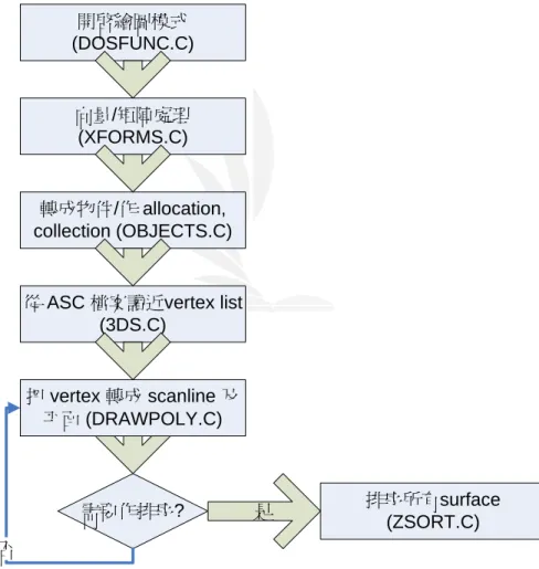
(8) 基本3D繪圖引擎使用Z排序演算法. Chapter 2. Engine Structure. 2.1 Introduction Basically, my engine relies upon the Z-Sort algorithm to draw a model onto the screen. Below is an architectural and file structure view of the engine. 開啟繪圖模式 (DOSFUNC.C). 向量/矩陣處理 (XFORMS.C). 轉成物件/作 allocation, collection (OBJECTS.C). 從 ASC 檔案讀近vertex list (3DS.C). 把 vertex 轉成 scanline 及平面 (DRAWPOLY.C). 需要作排序?. 是. 排序所有surface (ZSORT.C). 否. Figure 1 Architectural flowchart of engine structure. 8 逢甲大學 e-Paper (92學年度).

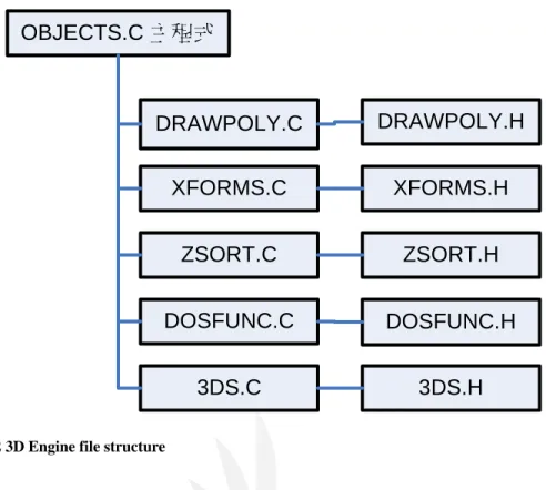
(9) 基本3D繪圖引擎使用Z排序演算法. OBJECTS.C 主程式. DRAWPOLY.C. DRAWPOLY.H. XFORMS.C. XFORMS.H. ZSORT.C. ZSORT.H. DOSFUNC.C. DOSFUNC.H. 3DS.C. 3DS.H. Figure 2 3D Engine file structure. As we can see, from a file-point-of-view, that the engine can be theoretically divided into five components, with each component taking care of a specific part of the rendering process. Here’s a brief summary of each component: OBJECTS.C: This is basically the main part of the engine. It handles management of objects, as well as the allocation and deallocation of resources used by said resources. DRAWPOLY.C:. This is where the almost everything is drawn. It. depends on having the edges initialized and sorted, and it takes care by pushing the priority surfaces to the front.. 9 逢甲大學 e-Paper (92學年度).

(10) 基本3D繪圖引擎使用Z排序演算法. XFORMS.C: This is where most of the vector math and projections are here. All data taken from a model file must undergo position and normal calculations. ZSORT.C:. This depth-sorting function determines which surfaces. or vertices need to be displayed. The algorithm uses radix sort to put the surfaces in order, and depending on the situation it puts the surfaces that need to be displayed on the front. DOSFUNC.C: Maintains some OS dependent functions. Since this engine runs on DOS, this is necessary. Because I have used neither DirectX nor OpenGL, the graphics calls must go through this procedure.. 2.2 Tools used for this project Here is a summary of the tools I have used for this project: Engine API: The basic skeleton structure of the engine, including the math functions was referenced from the Zed3D engine by Sebastien Loisel. 3D models: All of the 3D models I have used come from the internet. There are websites that provide 3D models of any kind free for download, such as http://www.3dcafe.com 10 逢甲大學 e-Paper (92學年度).

(11) 基本3D繪圖引擎使用Z排序演算法. Discreet 3D STUDIO MAX: I have only used this modeling program to convert from the .MAX binary format to the older .ASC ASCII format. Other than that, I have not used any of this programs’ functions. Microsoft Visual C++ 6.0: I used this to write my engine, which is pure C code. Zortech C++ compiler: I used this compiler because my graphics engine runs primarily on DOS and needed several privileged DOS system calls which the Visual C++ compiler could not provide.. 2.3 Main program steps The main program simply does the following: 1) Initialize memory 2) Allocate structure 3) Read data from file 4) Save data into structure 5) Loop until all data is stored into structure 6) Shutdown. Here are some of the more important data structures used for the main routine:. 11 逢甲大學 e-Paper (92學年度).

(12) 基本3D繪圖引擎使用Z排序演算法. void main(void) { o=read_3ds_file(“INPUTFILE",1); if(!o) { puts("Error reading file"); return; } A=B=C=0; for(a=0;a<o->pts_data->numpoints;a++) { A+=realtofloat(o->pts_data->vertex[a].location[0]); B+=realtofloat(o->pts_data->vertex[a].location[1]); C+=realtofloat(o->pts_data->vertex[a].location[2]); } A/=o->pts_data->numpoints; B/=o->pts_data->numpoints; C/=o->pts_data->numpoints; for(a=0;a<o->pts_data->numpoints;a++) { o->pts_data->vertex[a].location[0]-=floattoreal(A); o->pts_data->vertex[a].location[1]-=floattoreal(B); o->pts_data->vertex[a].location[2]-=floattoreal(C); } /* 分配空間給記憶體 pipeline */ pip=alloc_pipeline(300,700,2100); if(!pip) { puts("Memory allocation error"); return; } initmatrix(camera.m, 1,0,0, 0,1,0, 0,0,1); initvector(camera.v,0,0,3000); /* 分配空間給 buffer */ buf=init256(); if(!buf) { totxt(); puts("Memory allocation error"); return; } /* 一開始 polycount 設為 0 */ polycount=0; time0=clock(); do. 12 逢甲大學 e-Paper (92學年度).

(13) 基本3D繪圖引擎使用Z排序演算法. { reset_pipeline(pip); /* 記憶體 pipeline 清楚 */ cull_object(o,pip,&camera); /* 設 camera 成投影物件 */ sort_pipeline(pip); /* 把記憶體上物件作排序動作 */ memset(buf->buffer,1,buf->width*buf->height); for(a=pip->fptr-1;a>=0;a--) { f=pip->fbase+pip->index1[a]; pol.edgetable=edg; pol.color=realtofloat(mul(f->normal[2],floattoreal(30)))+70; for(b=0;b<3;b++) { p=&pip->pbase[f->index[b]]; edg[b].x1=realtofloat(p->scr_X)*500.0; edg[b].y1=realtofloat(p->scr_Y)*500.0; } pol.numedges=3; if(drawing) drawpolygon(&pol,buf); } blit(buf); mat_orthonormalize(camera.m); polycount+=o->face_data->numfaces; } while(!do_rotation(camera.m)); time1=clock(); /* 放出使用的記憶體 */ free256(buf); total_time=(time1-time0)/CLK_TCK; printf("Total time elapsed: %f seconds\nTotal # of polygon blitted: %li\nPolygons per second: %f\n\n", total_time,polycount,polycount/total_time); }. 13 逢甲大學 e-Paper (92學年度).

(14) 基本3D繪圖引擎使用Z排序演算法. Chapter 3 principles. Fundamentals and. 3.1 Introduction My engine uses the ASC export files as input. ASC files are ASCII description files for 3D models, and are used by the 3D Studio program. This is the first step in the engine process. I have used the 3D STUDIO ASCII file format for the 3D models. In case you were wondering, why didn’t I choose a more popular format like 3D STUDIO MAX or MAYA? Well below are the reasons: - ASCII file format is easier to understand than binary format. - It’s easier to learn the method by which triangles and polygons are generated. - It’s easier to write function that can read ASCII format. But it also has disadvantages as well, with speed and security being two of them.. 14 逢甲大學 e-Paper (92學年度).

(15) 基本3D繪圖引擎使用Z排序演算法. 3.2 How to read .ASC files The ASC file format requires several key fields: - Name object - Vertices - Faces - Vertex list - Position 3DS.C and 3DS.H take care of all model input. The underlying code shows how to read the vertex list and put it into a data structure. The data structure contains an index to the pointer array, the number of points and the vector normal.. struct face_struct { long *index; /* index 指到 pointer array */ long numpoints; vector normal; REAL D; /* Ax+By+Cz=D */ };. Below is the code for reading the vertex list. The resulting data is put into pts_data->vertex[i]->location[j]. if(read_line(s,f)) { free_object(o); return 0; } if(print_progress) { printf("Now reading file %s, %li vertices and %li faces.\n", filename,x,y); }. 15 逢甲大學 e-Paper (92學年度).

(16) 基本3D繪圖引擎使用Z排序演算法. for(a=0;a<x;a++) { if(read_line(s,f)) { free_object(o); return 0; } if(memcmp(s,"Vertex",6)) { a--; continue; } b=atol(s+7); if(print_progress) { if(!(a&127)) { printf("Vertex #%li\n",b); } } if(a!=b) { if(print_progress) puts("Vertex discrepancy"); free_object(o); return 0; } for(c=0;s[c]!='X';c++) {} A=strtod(s+c+2,0); for(;s[c]!='Y';c++) {} B=strtod(s+c+2,0); for(;s[c]!='Z';c++) {} C=strtod(s+c+2,0); o->pts_data->vertex[b].location[0]=floattoreal(A); o->pts_data->vertex[b].location[1]=floattoreal(B); o->pts_data->vertex[b].location[2]=floattoreal(C); }. 3.3 .ASC file structure and organization The file contents themselves are pretty straightforward. Here’s a section of a 3D model called DUCK.ASC.. 16 逢甲大學 e-Paper (92學年度).

(17) 基本3D繪圖引擎使用Z排序演算法. Ambient light color: Red=0.3 Green=0.3 Blue=0.3 Named object: "Object03" Tri-mesh, Vertices: 270 Faces: 516 Vertex list: Vertex 0: X: -28.091742 Y: -1166.367065 Z: -1902.944458 Vertex 1: X: 50.858582 Y: -1058.602417 Z: -1908.559204 Vertex 2: X: 103.18132 Y: -911.628906 Z: -1914.481323 Vertex 3: X: 122.565582 Y: -743.09613 Z: -1918.81897 Vertex 4: X: 106.673386 Y: -573.352966 Z: -1920.545776 Vertex 5: X: 57.421661 Y: -422.955139 Z: -1919.865356 Vertex 6: X: -19.249247 Y: -310.11795 Z: -1917.99231 Vertex 7: X: -114.091805 Y: -248.4814 Z: -1916.476685 Vertex 8: X: -124.147148 Y: -1222.063599 Z: -1899.620728 Vertex 9: X: 96.618271 Y: -1527.198608 Z: -1750.835693 Vertex 10: X: 244.996277 Y: -1328.9198 Z: -1767.286499. Description: Ambient light color: Here is the RGB values for ambient lighting. My engine does not read this value. It only assigns generic lighting. Background color: Here is the RGB values for the background color. My engine does not read this value. Named object: The object name. Can be any string value. Tri-mesh: Indicates model type. Vertices: The total number of vertices for this model Faces: The total number of triangle faces for this model Vertex list: Below is the list of X, Y, and Z coordinates relative to the center of the screen.. 3.4 Why choose .ASC files?. 17 逢甲大學 e-Paper (92學年度).

(18) 基本3D繪圖引擎使用Z排序演算法. The primary reason I chose ASC files is obviously because its contents can be easily read by a user. Today, many software packages prefer using the binary format over ASCII due to several reasons. 1) Binary format is faster than ASC format, especially when dealing with textures. 2) Binary format is much smaller than an equivalent ASC format. The number of vertex required for ASC format is great because there must specify X, Y, Z for every vertex. Binary format need only store the difference. 3) Binary format is the standard format used by many popular graphics APIs today, such as DirectX and OpenGL.. 18 逢甲大學 e-Paper (92學年度).

(19) 基本3D繪圖引擎使用Z排序演算法. Chapter 4. Rendering. 4.1 Introduction Rendering is the phase where we do the actual drawing. There is a general tendency to download this particular task to a slave graphics processor and leave the CPU to do better things. However, it will always be useful for everyone to have a general understanding of how things work. And also likely is the fact that we're going to need software renderers for a while more. And one last fact is that people have to write the software for the slave processor. We will first study the drawing of a point, which will be used to draw other primitives. Then we will study lines and polygons. Curved surfaces can also be supported but will not be discussed. The curved primitive that tend to be faster in drawing are conics and polynomials. However, some other forms of curved primitives definitions are often preferred, mainly splines.. 4.2 XFORMS subroutine. 19 逢甲大學 e-Paper (92學年度).

(20) 基本3D繪圖引擎使用Z排序演算法. XFORMS calculates all the vector and matrix mathematics. It contains the basic linear algebra operations (add, substract, multiply) for vectors and matrices, and it also adds normalization and orthonormalization. The following functions: Matrix addition void mat_add(matrix r, matrix a, matrix b) { int x,y; for(x=0;x<3;x++) for(y=0;y<3;y++) r[x][y]=add(a[x][y],b[x][y]); }. Matrix substraction oid mat_sub(matrix r, matrix a, matrix b) { int x,y; for(x=0;x<3;x++) for(y=0;y<3;y++) r[x][y]=sub(a[x][y],b[x][y]); }. Matrix multiplication void mat_mul(matrix r, matrix a, matrix b) { int x,y,z; for(x=0;x<3;x++) for(y=0;y<3;y++) { r[y][x]=floattoreal(0.0); for(z=0;z<3;z++) r[y][x]=add(r[y][x],mul(a[z][x],b[y][z])); } }. 20 逢甲大學 e-Paper (92學年度).

(21) 基本3D繪圖引擎使用Z排序演算法. Vector addition oid vec_add(vector r, vector a, vector b) { int x; for(x=0;x<3;x++) r[x]=add(a[x],b[x]); }. Vector substraction void vec_sub(vector r, vector a, vector b) { int x; for(x=0;x<3;x++) r[x]=sub(a[x],b[x]); }. Vector multiplication REAL vec_dot(vector a, vector b) { /* a * b = a[0]*b[0]+a[1]*b[1]+a[2]*b[2] */ REAL dot; int x; dot=floattoreal(0.0); for(x=0;x<3;x++) dot=add(dot,mul(a[x],b[x])); return dot; }. Vector normalization void vec_normalize(vector a) { REAL length; int x; #ifdef use_fixed do { #endif length=floattoreal(0.0); for(x=0;x<3;x++) length=add(length,mul(a[x],a[x])); length=SQRT(length); /* 取根號 */ #ifdef use_fixed. 21 逢甲大學 e-Paper (92學年度).

(22) 基本3D繪圖引擎使用Z排序演算法. if(length<=floattoreal(0.001)) vec_mul_scl(a,a,floattoreal(1000)); } while(length<=floattoreal(0.001)); #endif /* second divide each component of the vector by the length of the vector */ for(x=0;x<3;x++) a[x]=div(a[x],length); }. Matrix orthonormalization: void mat_orthonormalize(matrix a) { vector temp; /* 第一個向量作 normalize */ vec_normalize(a[0]); /* 使第二與第一項兩相正交 */ vec_mul_scl(temp, a[0], vec_dot(a[1],a[0]) ); vec_sub(a[1], a[1], temp ); /* 第二個向量作 normalize */ vec_normalize(a[1]); /* 第三項兩 = 第一 * 第二 */ vec_crs(a[2],a[0],a[1]); }. 4.3 DRAWPOLY subroutine The DRAWPOLY subroutine draws all the sorted edges onto the screen.. 22 逢甲大學 e-Paper (92學年度).

(23) 基本3D繪圖引擎使用Z排序演算法. Figure 3 Flowchart of DRAWPOLY procedure. void drawpolygon(polygon *poly, outbuffer *out) { long scanline,delta,mode,a;. init_edges(poly,out); sort_edges(poly,out);. if(poly->inactive.next) { /* 把 polygon scanline 轉成第一個 scanline */ scanline=poly->inactive.next->y1; /* 計算 scanline 的 delta 值 */ delta=mulwidth(scanline+out->maxy); poly->active.next=0;. /* 作回圈動作一直到結束為止 */. 23 逢甲大學 e-Paper (92學年度).

(24) 基本3D繪圖引擎使用Z排序演算法. update_lists(poly,scanline); while(poly->active.next) { update_intercept(poly); draw_spans(poly,out,delta); /* go to next scanline */ scanline++; delta+=out->width; update_lists(poly,scanline); } } }. 24 逢甲大學 e-Paper (92學年度).

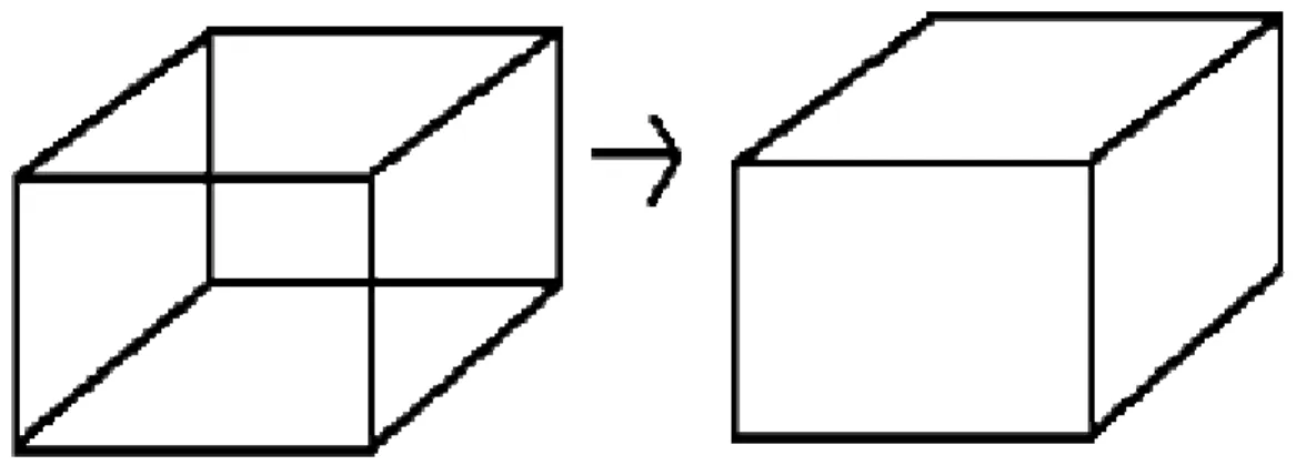
(25) 基本3D繪圖引擎使用Z排序演算法. Chapter 5 Visible Surface Determination 5.1 Introduction One of the problems we have yet to address, when several objects project to the same area on screen, how do you decide which gets displayed. Intuitively, the closest object should be the one to be displayed. Unfortunately, this definition is very hard to handle. We will usually say that the object to be displayed will be the one with the smallest z value in eye space, which is a bit easier to work with. A corollary of this is that objects with the largest 1/z value get displayed; this latter observation has applications which will be explained later.. Figure 4 Using Visible Surface Determination. 25 逢甲大學 e-Paper (92學年度).

(26) 基本3D繪圖引擎使用Z排序演算法. Visible surface determination can be done in a number of ways; each has its advantages, disadvantages and applications. Hidden line removal is used when wire frames are generated. This might be useful for a vector display, but will not be covered in here. When dealing with filled primitives, there are several classes of visible surface determination. There is also the question of object precision, device precision, and more, these topics will not be discussed here. Perhaps the most intuitive visible surface determination algorithm is the so-called "painter's algorithm", which works the same way a painter does. Namely, it draws objects that are further away first, and then draws objects that are closer. The advantage of this is it's simple. The disadvantages are that it writes several times to some areas of the display device, and also that some objects cannot be ordered correctly. The painter's algorithm can be generalized into the depth-sorting algorithm, which sort the primitives from back to front and then draw. The depth sorting algorithm also resolves cases that painter's algorithm does not.. 5.2 Sorting. 26 逢甲大學 e-Paper (92學年度).

(27) 基本3D繪圖引擎使用Z排序演算法. With the painter's algorithm, one has to assign a z-value to all primitives. Then, the primitives are sorted according these values of z, and the resulting image is drawn back-to-front. Several sorting algorithms can be used for this purpose, and even though basic algorithms are not the subject of this document, we will discuss two simple sorting schemes now. As can be seen, the algorithm is exceedingly simple. For small values of n (say, n<10), this algorithm can be used and will be close to optimal. However, if the list is very badly ordered initially, the sort could take up to n2 iterations before finishing. Small improvements can be made to the algorithm. For one thing, instead of always scanning in the same direction (from the first element to the last), one alternates directions, sorting an already close to sorted list is very efficient. The loop will execute roughly n times (actually, it would execute k times n, where k is some small constant). In the worse case though, it still executes in n2 iterations.. 5.3 Projection. 27 逢甲大學 e-Paper (92學年度).

(28) 基本3D繪圖引擎使用Z排序演算法. The projection technique I introduce here is back-face culling. Back-face culling exploits the observation that a face in a closed polyhedron always has two sides. One faces inside, and can never be seen by an observer outside the polyhedron (rather obviously since the polyhedron is closed), the other faces outside and can be seen. However, if it is determined that the side facing the eye is the inside of the face, that face will assuredly not be seen, because it is impossible to see a face from the inside.. Figure 5 Back-face culling from a left-handed system. VRP = Vertex Reference Point. Vector N = sum of three different vector in different coordinates of reference. The side that faces the eye can be determined easily with dot product. Take a vector V from the eye to any point within the polygon (for example, from the eye to a vertex). Let A be the normal of the polygon, assuming that A points outwards of the polyhedron. Then, compute V•A. If it is positive, the inside of the face is towards the camera, do not display or transform the face. If it is negative, the face is facing the camera and might be seen (though this is not guaranteed).. 28 逢甲大學 e-Paper (92學年度).

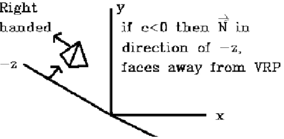
(29) 基本3D繪圖引擎使用Z排序演算法. Figure 6 Back-face culling from a right-handed system. VRP = Vector Reference Point. Back-face culling is generally not sufficient for visible surface determination. It is merely used to remove faces that assuredly cannot be seen. However, it will do nothing for faces that are only obscured by faces that are closer. Also, back-face removal assumes that the objects are closed polyhedra, and that faces are opaque. If this is not the case, back-face culling can not be applied.. Figure 7 Orthographic projection from back-face culling. 29 逢甲大學 e-Paper (92學年度).

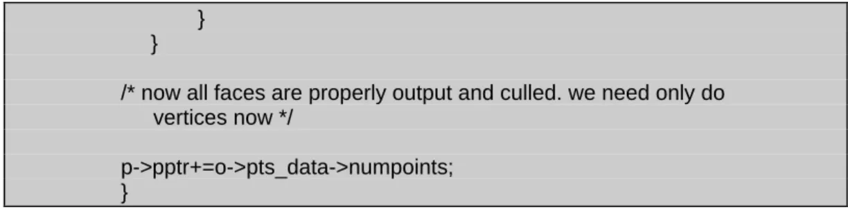
(30) 基本3D繪圖引擎使用Z排序演算法. Note that if the only thing displayed is a convex object, back-face culling is sufficient for visible surface determination (it will only leave the faces that are actually visible). void cull_object(object *o, pipeline *p, affine *xform) { long a,b,c,x,y,z; face *f,*g; pipe_point *pt; vector u; REAL D; pt=p->pbase+p->pptr; xform_pointcollection(o->pts_data,xform,pt); for(a=0;a<o->pts_data->numpoints;a++) { pt[a].point.clipping= o->pts_data->vertex[a].clipping; } f=o->face_data->face; for(a=0;a<o->face_data->numfaces;a++,f++) { /* backface cull. dot product of vector from eye to a point in face with normal vector of face */ mat_mul_vec(u,xform->m,f->normal); D=vec_dot(u, pt[*f->index].point.location); if(D>=floattoreal(0.0)) { /* clip */ for(b=0;b<f->numpoints;b++) pt[f->index[b]].point.clipping--; } else { /* output face to pipeline */ g=p->fbase+p->fptr;. g->index=p->ibase+p->iptr; g->numpoints=f->numpoints; copyvector(g->normal,u); g->D=D; for(b=0;b<f->numpoints;b++) g->index[b]=f->index[b]+p->pptr; /* update pointers */ p->iptr+=f->numpoints; p->fptr++;. 30 逢甲大學 e-Paper (92學年度).

(31) 基本3D繪圖引擎使用Z排序演算法. } } /* now all faces are properly output and culled. we need only do vertices now */ p->pptr+=o->pts_data->numpoints; }. 5.4 Painter's algorithm or Z-Sort As was previously mentioned, painter's algorithm assigns a z value to each primitive, then sorts them, then draws them from back to front. Objects that lie behind are then written over by objects that lie in front of them. Note that, no matter the scheme used to select the z value for an object, primitives that have overlap in z may be incorrectly ordered. But there is worse.. Figure 8 Easy and Difficult cases for the Painter's algorithm. 31 逢甲大學 e-Paper (92學年度).

(32) 基本3D繪圖引擎使用Z排序演算法. In this case, it is necessary to cut one triangle into two parts and sort the parts individually. Here is the pipeline sort procedure: long *sort_pipeline(pipeline *p) { long a,b,c; REAL A,B; face *f; pipe_point *pt; f=p->fbase; pt=p->pbase; for(a=0;a<p->fptr;a++,f++) { A=pt[f->index[0]].point.location[2]; B=A; for(b=1;b<f->numpoints;b++) { c=f->index[b]; if(pt[c].point.location[2]<A) A=pt[c].point.location[2]; else if(pt[c].point.location[2]>B) B=pt[c].point.location[2]; } p->index1[a]=a; p->minZ[a]=realtofixed(A); p->maxZ[a]=realtofixed(B); } bytesort(p->maxZ,p->index1,p->index2,p->fptr,0); bytesort(p->maxZ,p->index2,p->index1,p->fptr,1); bytesort(p->maxZ,p->index1,p->index2,p->fptr,2); bytesort(p->maxZ,p->index2,p->index1,p->fptr,3); return p->index1; }. Another sort that I have used is the byte_sort. #define getbyte(x,bitshift) (((x)>>(bitshift))&0xff) void bytesort(long *data, long *indexin, long *indexout, long itemcount, int bytenumber) { long count[257]; long a,b,c;. 32 逢甲大學 e-Paper (92學年度).

(33) 基本3D繪圖引擎使用Z排序演算法. for(a=0;a<=256;a++) count[a]=0; bytenumber*=8; for(a=0;a<itemcount;a++) { b=getbyte(data[indexin[a]],bytenumber); count[b+1]++; } for(a=1;a<256;a++) count[a]+=count[a-1]; for(a=0;a<itemcount;a++) { b=getbyte(data[indexin[a]],bytenumber); indexout[count[b]]=indexin[a]; count[b]++; } }. A way of handling all cases is as follows. Assign a z value to all polygons equal to the vertex belonging to the polygon that has the largest z coordinate value in eye space. Then sort as per painter's algorithm. Before actually drawing, we need to do a post sort stage to make sure the ordering is correct for polygons that have z overlap. Assuming we sorted in increasing values of z, it means that we need only to compare the last polygon with the consecutive previous polygons for which the furthest point is in the last polygon's z span. Once the last polygon is processed, we will not touch it anymore (unless the last polygon is moved to some other position in the list). Thus, we just consider the list to be one element shorter and recurse the algorithm. 33 逢甲大學 e-Paper (92學年度).

(34) 基本3D繪圖引擎使用Z排序演算法. Once a polygon has been moved in the list, mark it so that it is not moved again. If one of the above steps would say that a polygon that has already been moved in the list should be moved again, then you will have to use the last resort, clipping. Cutting up the triangle into pieces (clipping) will be described later. Of course, one needs not to perform all these tests if they are deemed to be more expensive than clipping. For instance, the only tests one could do is test for overlap in z, then x and y on screen, then check for step 2 and if it is still unresolved, simply clip the polygons and put the pieces where they belong. When polygon ordering can not be resolved, pick one of the two polygons for clipping plane and clip the other polygon with it. Then, insert the two pieces at the appropriate positions in the list. A very nice way of doing all these tests is as follows. Calculate bounding boxes for z value in 3d, and u,v in 2d (screen space, after perspective transform) of the polygon. Then, sort the bounding boxes in x, u and v. This can be done in linear time using the radix sort algorithm (or by exploiting coherence in a comparison sort algorithm). Then, only the polygons for which the bounding boxes overlap in all three axes need to be checked further. 34 逢甲大學 e-Paper (92學年度).

(35) 基本3D繪圖引擎使用Z排序演算法. Chapter 6 results. Engine testing and. 6.1 Testing the Engine I tested my engine against different 3D models of various sizes. They are listed below: Model file. Number of triangles. Number of vertices. THING.ASC. 48. 26. BALL.ASC. 68. 34. TORUS. 192. 96. DUCK.ASC. 516. 270. FACE.ASC. 1234. 656. Here is the sample result of executing program:. My test machine: CPU: AMD Athlon XP 2500+ Memory: 512 MB OS: Windows XP (To save space unnecessary space, I will only include the file contents for the first two model files) 35 逢甲大學 e-Paper (92學年度).

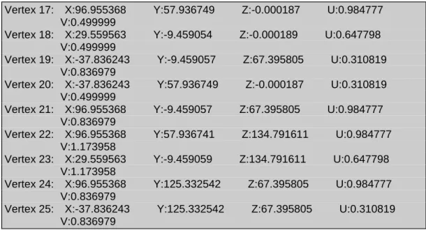
(36) 基本3D繪圖引擎使用Z排序演算法. THING.ASC Contents: Ambient light color: Red=0.078431 Green=0.078431 Blue=0.078431 Solid background color: Red=0 Green=0.001172 Blue=0.013162 Named object: "Light01" Direct light Position: X:56.75436 Y:-174.99263 Z:189.181213 Light color: Red=1 Green=1 Blue=1 Named object: "Camera01" Camera (48.235291mm) Position: X:421.18631 Y:-136.981934 Z:304.881714 Target: X:40.672749 Y:58.539715 Z:78.467651 Bank angle: 0 degrees Near 0 Far 1000 Named object: "B" Tri-mesh, Vertices: 26 Faces: 48 Mapped Vertex list: Vertex 0: X:-4.13834 Y:24.238838 Z:101.093712 U:0.479308 V:1.005469 Vertex 1: X:63.257465 Y:24.238838 Z:101.093704 U:0.816287 V:1.005468 Vertex 2: X:63.257462 Y:91.634834 Z:101.093704 U:0.816287 V:1.005468 Vertex 3: X:-4.138344 Y:91.634834 Z:101.093712 U:0.479308 V:1.005469 Vertex 4: X:-4.13834 Y:24.238842 Z:33.697807 U:0.479308 V:0.668489 Vertex 5: X:63.257465 Y:24.238842 Z:33.697807 U:0.816287 V:0.668489 Vertex 6: X:63.257462 Y:91.634644 Z:33.697811 U:0.816287 V:0.668489 Vertex 7: X:-4.138344 Y:91.634644 Z:33.697811 U:0.479308 V:0.668489 Vertex 8: X:29.559563 Y:57.936741 Z:134.791611 U:0.647798 V:1.173958 Vertex 9: X:29.559563 Y:-9.459057 Z:67.395805 U:0.647798 V:0.836979 Vertex 10: X:96.955368 Y:57.936745 Z:67.395805 U:0.984777 V:0.836979 Vertex 11: X:29.559563 Y:57.936749 Z:-0.000187 U:0.647798 V:0.499999 Vertex 12: X:29.559563 Y:125.332542 Z:67.395805 U:0.647798 V:0.836979 Vertex 13: X:-37.836243 Y:57.936745 Z:67.395805 U:0.310819 V:0.836979 Vertex 14: X:-37.836243 Y:57.936741 Z:134.791611 U:0.310819 V:1.173958 Vertex 15: X:29.559563 Y:125.332733 Z:134.791611 U:0.647798 V:1.173958 Vertex 16: X:29.559563 Y:125.332741 Z:-0.000184 U:0.647798 V:0.499999. 36 逢甲大學 e-Paper (92學年度).

(37) 基本3D繪圖引擎使用Z排序演算法. Vertex 17: Vertex 18: Vertex 19: Vertex 20: Vertex 21: Vertex 22: Vertex 23: Vertex 24: Vertex 25:. X:96.955368 V:0.499999 X:29.559563 V:0.499999 X:-37.836243 V:0.836979 X:-37.836243 V:0.499999 X:96.955368 V:0.836979 X:96.955368 V:1.173958 X:29.559563 V:1.173958 X:96.955368 V:0.836979 X:-37.836243 V:0.836979. Y:57.936749. Z:-0.000187. U:0.984777. Y:-9.459054. Z:-0.000189. U:0.647798. Y:-9.459057. Z:67.395805. U:0.310819. Y:57.936749. Z:-0.000187. U:0.310819. Y:-9.459057. Z:67.395805. Y:57.936741. Z:134.791611. U:0.984777. Y:-9.459059. Z:134.791611. U:0.647798. Z:67.395805. U:0.984777. Y:125.332542 Y:125.332542. Z:67.395805. U:0.984777. U:0.310819. Execution Results:. Figure 9 THING.ASC Polyhedron in wireframe. 37 逢甲大學 e-Paper (92學年度).

(38) 基本3D繪圖引擎使用Z排序演算法. Figure 10 THING.ASC Polyhedron in solid render. BALL.ASC Contents Ambient light color: Red=0.039216 Green=0.039216 Blue=0.039216 Named object: "Object01" Tri-mesh, Vertices: 114 Faces: 224 Vertex list: Vertex 0: X: 30.198587 Y: -82.96994 Z: 46.947147 Vertex 1: X: 63.860344 Y: -63.565693 Z: 43.373512 Vertex 2: X: 58.771538 Y: -58.101368 Z: 56.303982 Vertex 3: X: 48.9828 Y: -55.461559 Z: 67.2659 Vertex 4: X: 35.984379 Y: -56.048138 Z: 74.590424 Vertex 5: X: 21.755157 Y: -59.771812 Z: 77.162453 Vertex 6: X: 8.461412 Y: -66.065674 Z: 74.590424 Vertex 7: X: -1.873004 Y: -73.971558 Z: 67.2659 Vertex 8: X: -7.67477 Y: -82.285843 Z: 56.303982 Vertex 9: X: -8.060626 Y: -89.742767 Z: 43.373512 Vertex 10: X: -2.971826 Y: -95.207085 Z: 30.443045 Vertex 11: X: 6.816903 Y: -97.846901 Z: 19.481121 Vertex 12: X: 19.815331 Y: -97.260323 Z: 12.156591 Vertex 13: X: 34.044556 Y: -93.536659 Z: 9.584563 Vertex 14: X: 47.338303 Y: -87.242783 Z: 12.156595 Vertex 15: X: 57.672726 Y: -79.336906 Z: 19.481125 Vertex 16: X: 63.474483 Y: -71.022606 Z: 30.443056 Vertex 17: X: 87.799927 Y: -34.484135 Z: 33.196644 Vertex 18: X: 78.397057 Y: -24.387398 Z: 57.089039 Vertex 19: X: 60.309826 Y: -19.509659 Z: 77.344025 Vertex 20: X: 36.29187 Y: -20.593519 Z: 90.877975 Vertex 21: X: 9.999701 Y: -27.473963 Z: 95.630478 Vertex 22: X: -14.563936 Y: -39.103516 Z: 90.877975 Vertex 23: X: -33.659439 Y: -53.71167 Z: 77.344025 Vertex 24: X: -44.379715 Y: -69.074478 Z: 57.089043. 38 逢甲大學 e-Paper (92學年度).

(39) 基本3D繪圖引擎使用Z排序演算法. Vertex 25: Vertex 26: Vertex 27: Vertex 28: Vertex 29: Vertex 30: Vertex 31: Vertex 32: Vertex 33: Vertex 34: Vertex 35: Vertex 36: Vertex 37: Vertex 38: Vertex 39: Vertex 40: Vertex 41: Vertex 42: Vertex 43: Vertex 44: Vertex 45: Vertex 46: Vertex 47: Vertex 48: Vertex 49: Vertex 50: Vertex 51: Vertex 52: Vertex 53: Vertex 54: Vertex 55: Vertex 56: Vertex 57: Vertex 58: Vertex 59: Vertex 60: Vertex 61: Vertex 62: Vertex 63: Vertex 64: Vertex 65: Vertex 66: Vertex 67: Vertex 68: Vertex 69: Vertex 70: Vertex 71: Vertex 72: Vertex 73: Vertex 74: Vertex 75: Vertex 76: Vertex 77: Vertex 78:. X: -45.092686 X: -35.689804 X: -17.602591 X: 6.415371 X: 32.70755 X: 57.271191 X: 76.366707 X: 87.086975 X: 98.372787 X: 86.087326 X: 62.455227 X: 31.074257 X: -3.278118 X: -35.372059 X: -60.321537 X: -74.328255 X: -75.259789 X: -62.974339 X: -39.342247 X: -7.961272 X: 26.391113 X: 58.485062 X: 83.434555 X: 97.441254 X: 93.969269 X: 80.671585 X: 55.092388 X: 21.125866 X: -16.056873 X: -50.795101 X: -77.800232 X: -92.960983 X: -93.969276 X: -80.6716 X: -55.092407 X: -21.125885 X: 16.05687 X: 50.795109 X: 77.800247 X: 92.960991 X: 75.259773 X: 62.974312 X: 39.342216 X: 7.961252 X: -26.391119 X: -58.48505 X: -83.43454 X: -97.441246 X: -98.372787 X: -86.087334 X: -62.455242 X: -31.074274 X: 3.278112 X: 35.372055. Y: -82.853081 Z: 33.196655 Y: -92.949821 Z: 9.304267 Y: -97.827553 Z: -10.950727 Y: -96.743706 Z: -24.484695 Y: -89.863251 Z: -29.237181 Y: -78.233696 Z: -24.484688 Y: -63.625534 Z: -10.950726 Y: -48.262718 Z: 9.304283 Y: -0.152683 Z: 17.965897 Y: 13.039344 Z: 49.182812 Y: 19.412415 Z: 75.64724 Y: 17.996286 Z: 93.330193 Y: 9.006544 Z: 99.539627 Y: -6.188192 Z: 93.330193 Y: -25.274664 Z: 75.647232 Y: -45.347137 Z: 49.182816 Y: -63.349754 Z: 17.965902 Y: -76.541786 Z: -13.251005 Y: -82.914856 Z: -39.715431 Y: -81.498726 Z: -57.398399 Y: -72.508987 Z: -63.607838 Y: -57.31424 Z: -57.398399 Y: -38.227757 Z: -39.715424 Y: -18.155277 Z: -13.250981 Y: 34.202015 Z: 0.000001 Y: 48.480961 Z: 33.788944 Y: 55.379124 Z: 62.43383 Y: 53.846313 Z: 81.57373 Y: 44.115891 Z: 88.294769 Y: 27.669224 Z: 81.573723 Y: 7.010176 Z: 62.433826 Y: -14.716108 Z: 33.788944 Y: -34.202 Z: 0.000008 Y: -48.480949 Z: -33.788933 Y: -55.379108 Z: -62.433815 Y: -53.846306 Z: -81.57373 Y: -44.115887 Z: -88.294769 Y: -27.66921 Z: -81.573723 Y: -7.01015 Z: -62.433811 Y: 14.716146 Z: -33.788906 Y: 63.349762 Z: -17.965897 Y: 76.541794 Z: 13.251019 Y: 82.914856 Z: 39.715435 Y: 81.498726 Z: 57.398396 Y: 72.508995 Z: 63.607826 Y: 57.314255 Z: 57.398396 Y: 38.227783 Z: 39.715431 Y: 18.155312 Z: 13.251015 Y: 0.152702 Z: -17.965889 Y: -13.039324 Z: -49.1828 Y: -19.412399 Z: -75.647217 Y: -17.996273 Z: -93.330193 Y: -9.006536 Z: -99.539627 Y: 6.188209 Z: -93.330185. 39 逢甲大學 e-Paper (92學年度).

(40) 基本3D繪圖引擎使用Z排序演算法. Vertex 79: Vertex 80: Vertex 81: Vertex 82: Vertex 83: Vertex 84: Vertex 85: Vertex 86: Vertex 87: Vertex 88: Vertex 89: Vertex 90: Vertex 91: Vertex 92: Vertex 93: Vertex 94: Vertex 95: Vertex 96: Vertex 97: Vertex 98: Vertex 99: Vertex 100: Vertex 101: Vertex 102: Vertex 103: Vertex 104: Vertex 105: Vertex 106: Vertex 107: Vertex 108: Vertex 109: Vertex 110: Vertex 111: Vertex 112: Vertex 113:. X: 60.321552 Y: 25.274691 Z: -75.647217 X: 74.328247 Y: 45.347172 Z: -49.182774 X: 45.092678 Y: 82.853081 Z: -33.19664 X: 35.689804 Y: 92.949821 Z: -9.304252 X: 17.602575 Y: 97.82756 Z: 10.950741 X: -6.415382 Y: 96.743698 Z: 24.484695 X: -32.70755 Y: 89.863251 Z: 29.237181 X: -57.271191 Y: 78.233711 Z: 24.48469 X: -76.366692 Y: 63.625546 Z: 10.950739 X: -87.086967 Y: 48.262741 Z: -9.304249 X: -87.799942 Y: 34.484142 Z: -33.19664 X: -78.397064 Y: 24.387402 Z: -57.089027 X: -60.309841 Y: 19.509663 Z: -77.344025 X: -36.291882 Y: 20.593513 Z: -90.877975 X: -9.999702 Y: 27.473961 Z: -95.630478 X: 14.563941 Y: 39.103516 Z: -90.877975 X: 33.659458 Y: 53.711678 Z: -77.344017 X: 44.379719 Y: 69.074493 Z: -57.089008 X: 8.060633 Y: 89.742775 Z: -43.373508 X: 2.97183 Y: 95.207085 Z: -30.443031 X: -6.816909 Y: 97.846893 Z: -19.48111 X: -19.815334 Y: 97.260315 Z: -12.156584 X: -34.044556 Y: 93.536644 Z: -9.584553 X: -47.338299 Y: 87.242775 Z: -12.156585 X: -57.672718 Y: 79.336906 Z: -19.481112 X: -63.474487 Y: 71.022614 Z: -30.443035 X: -63.860344 Y: 63.565681 Z: -43.373497 X: -58.771542 Y: 58.101364 Z: -56.30397 X: -48.982807 Y: 55.461552 Z: -67.265892 X: -35.984379 Y: 56.04813 Z: -74.590424 X: -21.755156 Y: 59.771801 Z: -77.162453 X: -8.461406 Y: 66.065674 Z: -74.590424 X: 1.873016 Y: 73.971558 Z: -67.265892 X: 7.67478 Y: 82.285851 Z: -56.303959 X: -30.198587 Y: 82.96994 Z: -46.947147. Execution results:. 40 逢甲大學 e-Paper (92學年度).

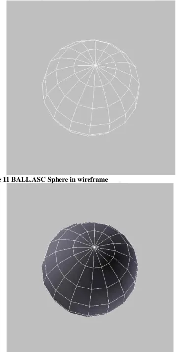
(41) 基本3D繪圖引擎使用Z排序演算法. Figure 11 BALL.ASC Sphere in wireframe. Figure 12 BALL.ASC Sphere in solid render. Execution results of TORUS.ASC:. 41 逢甲大學 e-Paper (92學年度).

(42) 基本3D繪圖引擎使用Z排序演算法. Figure 13 TORUS.ASC in wireframe. Figure 14 TORUS.ASC in solid render. Execution results of DUCK.ASC:. 42 逢甲大學 e-Paper (92學年度).

(43) 基本3D繪圖引擎使用Z排序演算法. Figure 15 DUCK.ASC Duck in wireframe. Figure 16 DUCK.ASC Duck in solid render. Execution results of FACE.ASC:. 43 逢甲大學 e-Paper (92學年度).

(44) 基本3D繪圖引擎使用Z排序演算法. Figure 17 FACE.ASC Face in wireframe. Figure 18 FACE.ASC Face in solid render. 6.2 Result Evaluation. I wanted to test the performance of z-sort algorithm versus more 44 逢甲大學 e-Paper (92學年度).

(45) 基本3D繪圖引擎使用Z排序演算法. modern algorithms by comparing the run time of each model, and seeing which runs the fastest. Unfortunately I could not find more complex models than these, because the ASC format is very old, and very few packages support it. Most formats I have seen are the .3DS and .MAX formats. As far as the rendering goes, Z-Sort does a decent job of rendering the surfaces as long as the models are not too complex. The highest polygon model I have used is only 1234 faces big, and since I have tested it on a modern computer with a fast processor, any attempt to differentiate the performance is negligible. To notice a performance decrease would require a model in the 100,000s of faces, which I could not find unfortunately.. 45 逢甲大學 e-Paper (92學年度).

(46) 基本3D繪圖引擎使用Z排序演算法. Conclusion With this research project I have understood the principles behind the rendering of an image onto the screen. The Z-sorting algorithm is a very simple algorithm compared to more modern implementations, and also very inefficient. As we have demonstrated earlier, it is not suitable for any large-scale and polygon intensive models, but it handles simple models fairly fast. The Z-buffer algorithm is currently the most used method and also the most efficient. Nearly all 3-D accelerators on the market support z-buffering, making z-buffers the most common type of depth buffer today. However ubiquitous, z-buffer tend to have the following drawbacks: Due to the mathematics involved, the generated z values in a z-buffer tend not to be distributed evenly across the z-buffer range (typically 0.0 to 1.0, inclusive). Specifically, the ration between the far and near clipping planes strongly affects how unevenly z values are distributed. Using a far-plane distance to near-plane distance ratio of 100, 90% of the depth buffer range is spent on the first 10% of the scene depth range. Typical applications for entertainment or visual simulations with exterior scenes often require far plane/near plane ratios of anywhere between 1000 to 10000. At a ratio of 1000, 98% of the range is spent on the 1st 2% of the 46 逢甲大學 e-Paper (92學年度).

(47) 基本3D繪圖引擎使用Z排序演算法. depth range, and the distribution gets worse with higher ratios. This can cause hidden surface artifacts in distant objects, especially when using 16-bit depth buffers (the most commonly supported bit-depth).. 47 逢甲大學 e-Paper (92學年度).

(48) 基本3D繪圖引擎使用Z排序演算法. Bibliography [1]. Alan Watt, Fabio Policarpo. 3D Games Real-time Rendering and Software Technology. ACM Press, 2001.. [2]. James D. Foley, Andries van Dam, Steven K. Feiner, John F. Hughes. Computer Graphics Principles and Practice. Addison-Wesley, 1997.. [3]. LaMothe, A. Tricks Of The Windows Game Programming Gurus, 2nd Ed. Sams Publishing, 2002.. [4]. Thomas H. Cormen, Charles E. Leiserson, Ronald L. Rivest, Introduction to Algorithms. McGraw-Hill, 1998.. [5]. S. D. Conte, Carl de Boor. Elementary Numerical Analysis. McGraw-Hill, 1980.. [6]. Ming Chieh Lin, Efficient Collision Detection for animation and robotics, PhD Thesis at University of California at Berkeley, 1993.. [7]. Barsky, B., Computer Graphics and Geometric Modeling Using Beta-splines, Springer-Verlag, New York, 1988.. 48 逢甲大學 e-Paper (92學年度).

(49)