國立交通大學
電機與控制工程學系
碩士論文
應用於眼球機器人之智慧型多軸追蹤控制
Intelligent Multiaxial Tracking Control Applied To
the Eye-Robot
研 究 生:徐傳源
A
指導教授:陳永平 教授
中 華 民 國 九 十 九 年 七 月
應用於眼球機器人之智慧型多軸追蹤控制
Intelligent Multiaxial Tracking Control Applied To
the Eye-Robot
研 究 生:徐傳源 Student:Joseph Sii Tuong Guan
指導教授:陳永平 Advisor:Yon-Ping Chen
國 立 交 通 大 學
電 機 與 控 制 工 程 學 系
碩 士 論 文
A Thesis
Submitted to Department of Electrical and Control Engineering
College of Electrical and Computer Engineering
National Chiao Tung University
in Partial Fulfillment of the Requirements
for the Degree of Master
in
Electrical and Control Engineering
July 2010
Hsinchu, Taiwan, Republic of China
i
應用於眼球機器人之智慧型多軸
追蹤控制
學生: 徐傳源 指導教授: 陳永平 教授
國立交通大學電機與控制工程學系
摘 要
為了模仿人類雙眼視覺的追蹤,本篇論文針對目標物的追蹤控制設計了結合 類神經網路的雙眼機器人。整個追蹤控制的策略可分為四個部分,首先是由雙眼 機器人利用攝影機擷取移動目標的影像,並且判別它的位置所在。其次是設計目 標位置中心和追蹤速度的關係當作脖子和眼睛的兩種訓練模式。接著再利用倒傳 遞演算學習法則的離線學習(off-line training)來設計四種類神經網路,學習訓 練模式所描述的目標位置中心對應速度之間的關係。最後,雙眼機器人採用了最 佳的訓練結果做為它的控制器來追蹤移動的目標。這些智慧型的追蹤控制器經由 實驗證明確實可成功地完成物體的定點追蹤控制和水平追蹤控制。ii
Intelligent Multiaxial Tracking Control
Applied To the Eye-Robot
Student:Joseph Sii Tuong Guan
Advisor:Prof.Yon-Ping Chen
Department of Electrical and Control Engineering
National Chiao Tung University
ABSTRACT
To emulate the humanoid binocular vision tracking, this thesis presents the tracking controller design based on the neural network for the Eye-robot to trace a moving object. The tracking control strategy is partitioned into four parts. First, the Eye-robot retrieves the image of the moving object from two cameras and identifies its position. Second, two training patterns concerning the relationship between the tracking velocity and object position are designed for the neck and two eyes to learn. Third, under off-line training four neural networks are constructed and trained by the back-propagation algorithm to learn the training patterns. Finally, the Eye-robot adopts the well trained neural networks as its controller to trace the moving object. The success of the tracking control of the Eye-robot can be concluded from the experiment results of the set-point control and the horizontal trajectory tracking control.
iii
Acknowledgement
誠摯感謝指導教授陳永平老師在這兩年中的悉心指導與教誨,老師嚴謹的治 學態度,理論與實務並重的訓練,使得本論文得以順利完成。在待人處事方面的 啟發更是讓我獲益良多,這份師恩會令我永生難忘。同時也感謝口試委員楊谷洋 教授與蔡尚澕教授對本論文所提出的珍貴意見與指正,讓本論文能更加的完整。 除此之外,感謝可變結構控制實驗室的承育、楊庭和新光學長們,瑋哲以及 學弟文榜、澤翰、文俊們在課業與研究上一起學習與勉勵,以及實驗上的協助, 也感謝你們在生活中帶給我的許多歡笑,使我的生活更多姿多彩,讓我在實驗室 的兩年研究生活變的歡樂與溫馨。此外,感謝世宏學長、桓展學長平日在攻讀博 士學位之餘,不吝傳授知識與經驗及給予建議。 最後,更感謝我親愛的父親、舅舅、哥哥、姊姊及表妹們,你們的關心與鼓 勵,給了我許多的溫暖,由於你們的支持,使我能專心在學習領域上衝刺,更感 激我已故的母親,因為有您,才有現在的我,真的很懷念您。最後再次由衷的謝 謝所有支持、關心與幫助過我的人。 謹以此篇論文獻給所有關心我、照顧我的人,你們的恩惠我銘感於心,由衷 感謝你們。 徐傳源 2010.7iv
Contents
Chinese Abstract...i
English Abstract...ii
Acknowledgement ... iii
Contents ...iv
List of Figures ...vi
List of Tables ...ix
Chapter 1 Introduction ... 1
1.1 Motivation ... 1
1.2 Related Work………... 2
1.3 Thesis Organization ... 5
Chapter 2 Intelligent Learning Algorithm... 6
2.1 Introduction to ANN ... 6
2.2 Back-Propagation Network ...10
Chapter 3 System Description ... 16
v
3.2 Hardware ...18
3.3 Software ...20
Chapter 4 Intelligent Object Tracking Controller Design ... 22
4.1 Object Detection ... 22
4.2 Tracking Control Design ...27
Chapter 5 Experimental Results ... 36
5.1 Neural Network Off-line Training ... 36
5.2 Set Point Control ... 39
5.3 Horizontal Object Tracking Control ... 45
Chapter 6 Conclusions and Future Work ... 54
vi
List of Figures
Figure 2.1 Schematic view of a neuron ... 7
Figure 2.2 Basic element of artificial neural network ... 7
Figure 2.3 Multilayer feed-forward network ... 9
Figure 2.4 Back-propagation network ... 11
Figure 2.5 Back-Propagation Cycle ...12
Figure 2.6 Flow chart of the design process of the back-propagation ...15
Figure 3.1 Whole system framework of the Eye-robot tracking...17
Figure 3.2 Eye-robot system ...19
Figure 3.3 Definition of axes of the Eye-robot ...20
Figure 4.1 RGB color space and the color cube. ...23
Figure 4.2 Image in RGB space ...25
Figure 4.3 Image transform to gray level ...25
Figure 4.4 Intensity of gray level distribution ...26
Figure 4.5 Binary image of taking the threshold as 180...26
Figure 4.6 Gray level image distribution ...27
vii
Figure 4.8 Eye training pattern ...28
Figure 4.9 Neck training pattern ...28
Figure 4.10 Structure of neck neural network ...31
Figure 4.11 Structure of left eye neural network ...32
Figure 4.12 Structure of left eye combine with neck neural network ...32
Figure 4.13 Structure of left eye combine with neck and right eye neural network ....33
Figure 4.14 Block diagram of the Eye-robot visual tracking control design architecture ...35
Figure 5.1 Set-point control of NNeye results of the left eye...40
Figure 5.2 Set-point control of NNeye results of the right eye ...40
Figure 5.3 Set-point control of NNneck results of the neck ...41
Figure 5.4 Set-point control of NNeye1-neck results of the left eye combine with neck .42 Figure 5.5 Set-point control of NNeye results of the right eye ...42
Figure 5.6 Set-point control of NNeye2-neck results of the left eye combine with neck and right eye ...43
Figure 5.7 Set-point control of C3NN errors result ...44
Figure 5.8 Set-point control of C2NN errors result ...44
viii
Figure 5.10 6 seconds of C3NN errors tracking control result ...46
Figure 5.11 6 seconds of C2NN errors tracking control result ...47
Figure 5.12 6 seconds of C1NN errors tracking control result ...47
Figure 5.13 9 seconds of C3NN errors tracking control result ...49
Figure 5.14 9 seconds of C2NN errors tracking control result ...49
Figure 5.15 9 seconds of C1NN errors tracking control result ...50
Figure 5.16 12 seconds of C3NN errors tracking control result ...50
Figure 5.17 12 seconds of C2NN errors tracking control result ...51
Figure 5.18 12 seconds of C1NN errors tracking control result ...51
Figure 5.19 15 seconds of C3NN errors tracking control result ...52
Figure 5.20 15 seconds of C2NN errors tracking control result ...52
ix
List of Tables
Table 5.1 Neck neural network off-line training parameter...37
Table 5.2 Eye neural network off-line training parameter ...37
Table 5.3 Left eye combine with neck neural network off-line training parameter ...38
Table 5.4 Left eye combine with neck and right eye neural network off-line training parameter ...38
1
Chapter 1
Introduction
In recent years, computer graphics technology has witness considerable developments. Because of the increased capabilities of the central processing unit (CPU), it is possible to process a large amount of data within a short time. Previously because graphics data was too large to handle, it become necessary to increase the speed of image systems processing by manufacturing more advance of CPUs or by developing more powerful graphics processing system.
In this study, a fast and effective Eye-robot tracking is developed. The two eyes (webcams) of the Eye-robot connected over the Universal Serial Bus (USB) interface for image input to build an image tracing system. The major function of this Eye-robot tracking is to rapidly track an object and determine its plane coordinates. This system measures the 2D coordinates of an object using the spatial relationships between two webcams and the object. A servo motor produces a pulse signal in accordance with the tracked coordinate to maintain the object at the center of the images.
1.1 Motivation
Computer vision and image processing are popular research fields owing to their wide varieties of application such as military industry, satellite system, medical equipment, video conference, and human recognition are also common use of computer vision in our daily lives. Among all of these applications, visual tracking, for example, object motion tracking, has become a great interest in this domain. Object tracking is important because it enables several important applications such as:
2
Security and surveillance – to provide better sense of security using visual information; Medical therapy – to improve the quality of life for physical therapy patients and disabled people; Traffic management – to analyze flow, to detect accidents; Videos editing – to eliminate cumbersome human-operator interaction, to design futuristic video effects. This thesis introduces an efficient approach of a real-time moving object tracking by the two eyes of the Eye-robot and describes the design of an algorithm based on the neural network structure to deal with this problem and the implementation of the visual servo control system to achieve this purpose.
1.2 Related Work
The problem of the Eye-robot object tracking has already been treated in various forms and has led to the development of many methods. In general, there has one major scheme, image-based visual servo control for the Eye-robot tracking. In this control, an error signal is measured in the image and mapped directly to actuator command. This strategy is also called vision feedback control. A vision-based control overcomes many difficulties of uncertain models and unknown environments. A typical example of an image-based system is consisting of a camera and an object information processing unit that provides the feedback information for the servo control. Thus, the speed of capturing an image must be as fast as possible to detect the move of the object in real-time. However, the camera has a constraint on the number of capturing image per second.
In many object tracking systems that have been developed, the hardware architecture is based on two processors, one digital signal processor for the image processing, and the other controller for the Eye-robot control. The purpose of utilizing bi-processor system is in order for efficiency. Otherwise, there are many approaches
3
based on PC because of its capability and facility.
Many approaches for object detection are used for surveillance systems that have been developed to monitor real environments, e.g. airport, highway, and station, etc. Moreover, an object motion tracking is of an interest in numerous applications. Using a distributed camera system to detect the object motion in different viewpoints and using a multi-class model of color to obtain a 2D representation of object is an example for the object tracking. The ability to find and follow the motion of the object is therefore an important visual problem to research. This thesis proposes a color detection strategy to detect the object and its position of an image to achieve the Eye-robot tracking. Finally, computing the center of gravity is to obtain the object position. During the Eye-robot tracking, the background must be pure in whole tracking.
For servo control system, the proportional plus integral (PI) controller is still the most widely used for motor control due to its relatively simple implementation. The fixed gain feedback control is based on an accurate system model. However, PI control method is not robust enough to accommodate the external disturbances (torque load), parameter variations, and structural controller that can self-tune its control gains according to the variations in operating conditions. This will take advantage of its simplicity and feasibility. The parameters of the controller are updated on-line to achieve a specified dynamic response, thus, self-tuning control techniques are being recognized as promising methods. A self-tuning PI strategy is proposed for speed control with load torque compensation. Besides, a self-tuning for reference tracking is also available to drive a DC motor.
Recently, much research has been carried out to apply the neural network to control field in order to deal with nonlinearities and uncertainties of the control system. The neural network technique is a better alternative for the modeling and
4
control of complex nonlinear systems because of its high learning and nonlinear mapping ability. This method has been successfully applied to MCDC 3006S motor control systems. Besides, a hybrid controller, which combines the advantages of the PI controller and neural network, is proposed to compensate for the uncertainties of the MCDC 3006S servo motor to drive in both position and speed control for the Eye-robot.
Back-propagation neural network are the most prevalent neural network architectures for adaptive control applications because they have the capability to learn system characteristics through nonlinear mapping. This thesis proposes a neural network training control system applying the back-propagation algorithm for MCDC 3006S motor drive.
This thesis integrates the image processing for object detection and the servo control of the Eye-robot for the object tracking to achieve a visual Eye-robot tracking system. The system, which works in real-time, is able to detect, localize, and track the object moving in the scene. The idea is to put an object anywhere in the scene and for the Eye-robot to detect the object and trace the object in the center. Besides, if the object is moving, the Eye-robot will keep the object in the center.
During the computer simulations, the proposed approach is executed to verify its feasibility in different conditions. In real experiments, a PC-based system with RS-232 interface is used to carry out the tasks. The RS-232 interface card with a DC-servomotor of MCDC 3006S motor control is developed in this thesis and implemented in this experiment.
5
1.3 Thesis Organization
This thesis deals with object tracking, and the rest of the thesis is organized as follows. The intelligent learning algorithm of the back-propagation will be introduced in Chapter 2. In Chapter 3, we represented the system problem statement concepts related to the object tracking, and the system hardware and software will be described. Chapter 4 deals with object detection and intelligent object tracking controller design, which we implemented for object tracking, provides a detailed description of the Eye-robot tracking. In Chapter 5 experimental results and discuss are provided. At last, the conclusions and future work will be proposed in Chapter 6.
6
Chapter 2
Intelligent Learning Algorithm
This chapter discusses a popular learning method capable of handling such large learning problem, which is back-propagation learning algorithm. This algorithm can be efficiently implemented in computing system in which only local information can be transported through the network. The detailed explanation about intelligent learning algorithm will be introduced in the section. Section 2.1 introduces the artificial neural network (ANN), which is introduces the neuron that mimic human nervous. Section 2.2 describes a kind of neural network learning algorithm, which is the back-propagation network learning algorithm.
2.1
Introduction to ANN
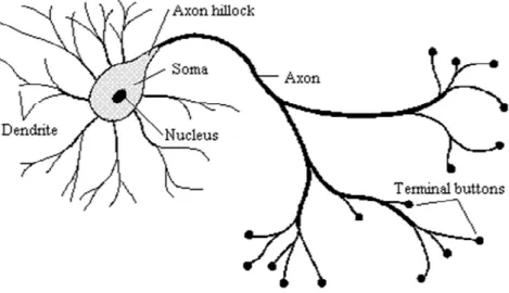
The human nervous system consists of a large amount of neurons, shown in Figure 2.1, including somas, axons, dendrites and synapses. Each neuron is capable of receiving, processing, and passing electrochemical signals from one to another. In order to mimic the characteristics of the human nervous system, recently investigators have developed an intelligent algorithm, called artificial neural network (ANN), to construct intelligent machines capable of parallel computation. This thesis will apply ANN to learn the object tracking of the Eye-robot.
7
.
.
.
.
.
.
y xn x3 x2 x1 b wn w3 w2 w1
f(.)
Figure 2.2 Basic element of artificial neural network Figure 2.1 Schematic view of a neuron
8
As shown in Figure 2.2, the basic element of ANN has N inputs and each input is multiplied by a corresponding weight, analogous to synaptic strengths. The weighted inputs and the bias are summed to determine the activation level of the neuron, whose input-output relation is expressed as
1 n i i i y f w x b
(2.1-1)where wi is the weight at the input xi and b is the bias. The behavior of an ANN
depends on the weights, bias and activation function specified for each neuron. The activation function f(․) is usually chosen to be one of the following fundamental forms (1) Step function: 0 0 0 1 ) ( v if v if v f (2.1-2) (2) Piecewise-linear function: v v if v v v if v v v v v v if v f 2 1 2 2 1 2 1 0 1 ) ( (2.1-3) (3) Sign function: 0 1 0 1 ) ( v if v if v f (2.1-4) (4) Sigmoid function: 0 , 1 1 ) ( c e v f cv (2.1-5)
In this thesis, the sigmoid function in (2.1-5) is used as the activation function since it is very similar to the input-output relation of biological neurons. The commonest multilayer feed-forward network, constructed by the basic element, is
9
shown in Figure 2.3 Multilayer feed-forward network 2.3, which contains input layer, output layer, and hidden layer. A multi-hidden layer network can solve more complicated problems than a single-hidden layer network. However, the training process of multi-hidden layer is more difficult. The numbers of hidden layers and their neurons are decided by the complexity of the problem to solve.
In addition to the architecture, the method of setting the weights is an important matter for a neural network. For convenience, the learning for a neural network is mainly classified into two types, supervised and unsupervised. The training in supervised learning is mapping a given set of inputs to a specified set of target outputs. The weights are then adjusted according to various learning algorithms. For unsupervised learning, a sequence of input vectors is provided, but no target vectors are specified. The network modifies the weights so that the most similar input vectors
Output layer Input layer 2nd hidden layer 1st hidden layer
.
.
.
.
.
.
.
.
.
.
.
.
.
.
10
are assigned to the same output unit. In this thesis, the neural network learns the behavior by input-output pairs, a way of supervised learning.
2.2 Back-Propagation Network
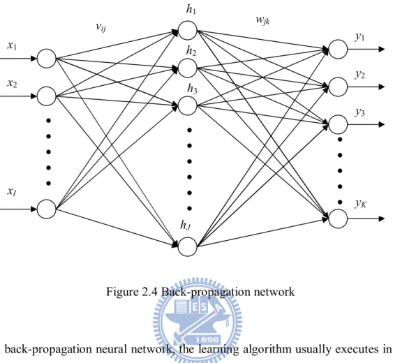
In supervised learning, the back-propagation network learning algorithm is widely used in most applications. The back-propagation algorithm was proposed in 1986 by Rumelhart, Hinton and Williams, which is based on the gradient descent method for updating the weights to minimize the total square error of the output. The training by the back-propagation algorithm is mainly applied to multilayer feed-forward network in three steps: input training patterns, calculate errors via back-propagation, and adjust the weights accordingly. Figure 2.4 shows the back-propagation network, including input layer with I neurons, one hidden layer with Jneurons and output layer with Kneurons. Let xi be the input to the i-th neuron of the
input layer, i=1,2,…,I. For the output layer, the output of the k-th neuron, k=1,2,…,K, is expressed as ,..., 2 , 1 , 1 K k h w f y J j j jk k k
(2.2-1)where fk(・) is the activation function related to the k-th neuron and wjk is the weight
from the j-th neuron in the hidden layer to j-th neuron in the output layer. As for the hidden layer, the output of its j-th neuron is obtained as
,..., 2 , 1 , 1 J j x v g h I i i ij j j
(2.2-2)where gj(・) is the activation function related to the j-th neuron and vij is the weight
11
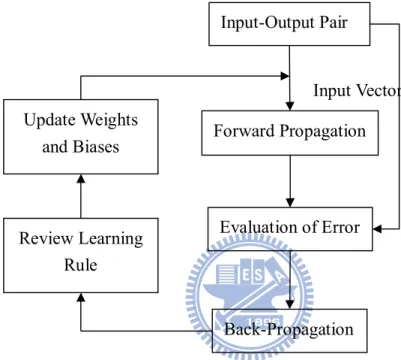
In a back-propagation neural network, the learning algorithm usually executes in two phases. First, a training input pattern is presented to the network input layer, and propagated through hidden layer to output layer, which generates an output pattern. If this pattern is different from the desired output, an error is calculated and then propagated backward from the output layer to the input layer. The weights are modified as the error is propagated. The back-propagation training is designed to minimize the mean square error between the actual output and the desired output, which is based on an iterative gradient algorithm. A learning cycle starts with applying an input vector to the network, which is propagated in a forward propagation mode which ends with an output vector. Next, the network evaluates the errors between the desired output vector and the actual output vector. It uses these errors to shift the connection weights and biases according to a learning rule that tends to
y3 h3 x2 x1
.
.
.
.
.
.
.
.
.
.
.
.
.
.
.
.
y2 y1 h2 h1 xI hJ yK vij wjk12
minimize the error. This process is generally referred to as “error back-propagation” or back-propagation for short. The adjusted weights and biases are then used to start a new cycle. A back-propagation cycle, also known as an epoch, in a neural network is illustrated in Figure 2.5. For a finite number of epochs the weights and biases are shifted until the deviations from the outputs are minimized.
The learning algorithm of the back-propagation is elaborated on as below:
Step 1: Input the training data.
The training data contain a pair of input x[x1 x2xI ]T and desired
output T
K
d d d
d [ 1 2 ] . Set appropriate maximum tolerable error Emax and leaning rate between 0.1 and 1.0, according to the computing time and the precision.
Step 2: Randomly set the initial weights and bias values of the network. Step 3: Calculate the outputs of the hidden layer and the output layer.
Input-Output Pair Forward Propagation Evaluation of Error Back-Propagation Review Learning Rule Update Weights and Biases Input Vector Output Vector (Target)
13
Step 4: Calculate the error function expressed as
K k J j j jk k k K k k k h w f d y d E 1 2 1 1 2 2 1 2 1 (2.2-3)where yk is the actual output and dk is the desired output.
Step 5: According to the gradient steepest descent method, determine the
correction of weights as
j jk j J j j jk k k k jk k k jk jk h h h w f y d w y y E w E w
1 ' (2.2-4) and
i ijk i I i i ij j jk J j j jk k k k ij j j k k ij ij x x x v g w h w f y d v h h y y E v E v
1 ' 1 ' (2.2-5) where
J j j jk k k k jk d y f w h 1 '
I i i ij j jk J j j jk k k k ijk d y f w h w g v x 1 ' 1 ' .Step 6: Propagate the correction backward to update the weights as below
ij ij ij jk jk jk v n v n v w n w n w 1 1 (2.2-6)14
Step 7: Check whether the whole training data set have learned or not.
When the network has learned the whole training data set, it is called that the network goes through a learning cycle. If the network does not go through a learning cycle, return to Step 1, otherwise, go to Step 8.
Step 8: Check whether the network converges or not.
If E<Emax, terminate the training process, otherwise, begin another
learning cycle by going to Step 1.
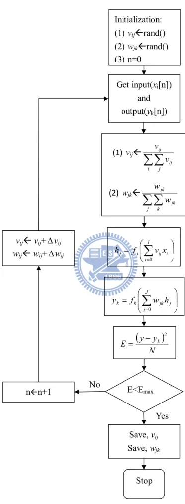
Back-propagation network learning algorithm can be used to model various complicated nonlinear functions. Recently the back-propagation network learning algorithm is successfully applied to many domains and applications, such as pattern recognition, adaptive control, clustering problem, etc. In this thesis, the back-propagation network algorithm was used to learn the relationship between input (position) and output (velocity) function for the eye-robot to pursuit an object. Figure 2.6 shows the flow chart of the design process of the back-propagation algorithm.
15 Get input(xi[n]) and output(yk[n]) (1) vij
i j ij ij v v (2) wjk
j k jk jk w w
I i i ij j j f v x h 0 E<Emax No Yes Stop vij vij+ vij wij wij+ wij Save, vij Save, wjk Initialization: (1) vijrand() (2) wjkrand() (3) n=0
J j j jk k k f w h y 0
N y y E k 2 nn+116
Chapter 3
System Description
The Eye-robot designed for object tracking can be viewed as an integration of three subsystems, including a humanoid visual system (HVS), an image processing system (IPS) and a tracking control system (TCS). The HVS is constructed by two cameras in parallel to emulate the human eyes and detect the object. The IPS is used to abstract the features of the object from the images retrieved by the HVS. After the object features are recognized, the TCS is then adopted to drive the HVS to track the object. This chapter will focus on the design of the TCS based on the back-propagation neural network.
3.1 Problem Statement
This section describes the humanoid visual system (HVS), an image processing system (IPS) and a tracking control system (TCS). The HVS is built with two cameras and five motors to emulate human eyeballs. The IPS is first transformed the image retrieved from the Eye-robot into a gray level image, and then taking a threshold can be easily selected for the object. The TCS is the mainly part for this thesis used in the Eye-robot tracking control, which is the controller via the off-line training with the used of neural network. There are four neural networks used in this thesis, including NNneck, NNeye, NNeye1-neck, and NNeye2-neck. With these four neural networks, there are three types of tracking control, which are C3NN, C2NN and C1NN. Then the off-line training results will be compared with these three types of tracking control. When the object location in the two cameras image is obtained and determined, the purpose of object tracking can be achieved by the Eye-robot.Here is a
17
brief describes to the object detection method and the tracking control of the Eye-robot, and how to obtain the space coordinates of the Eye-robot will be introduced in Chapter 4.
The Eye-robot is a challenging and important problem in computer vision. The Eye-robot tracking is expected to detect the position of an object in a scene and maintain its position in the center of the image plane. How to design and maintain a high performance of the control system is an important topic for sturdy.
In this thesis, an object is tracked by the Eye-robot. The object is projected by an overhead projector in a screen. The speed of the object motion velocity is 28 cm/sec. The distance between the Eye-robot and screen are designed around 240 cm and the proportion of the vision object in the Eye-robot is designed as 10cm10cm.
Figure 3.1 shows the whole system framework of the Eye-robot tracking, it includes camera, graphic-card, personal desktop, RS 232 interface transmission and MCDC controller for the most part to construct the close-loop of the Eye-robot tracking system.
Object Camera Graphic
Card Personal Desktop RS232 Interface MCDC Controller Eye-robot Position Image Signal Digital Image Control Signal Voltage Signal Image Tracking
Figure 3.1 Whole system framework of the Eye-robot Tracking
ASCII Control
18
3.2 Hardware
The Eye-robot tracking system is built with two cameras and five motors to emulate human eyeballs as shown in Figure 3.2. This active vision head of the Eye-robot was designed to mimic the human visual system. The hardware used in Eye-robot tracking using include motor controller, one desktop computer, power supply, two cameras, several I/O port and motor drive cards are used to implement the overall Eye-robot tracking system.
The Eye-robot adopts five FAULHABER DCservomotors to steer the Eye-robot in tracking system. Each motor works at voltage 15V, frequency 31.25 kHz, maximum output current 0.35 A and maximum speed 15000 rpm. With RS-232 interface, the controller of DCservomotors is executed by the motion control card, MCDC 3006S, in a positioning resolution of 0.18°. With these 5 degrees of freedom, the object tracking system would track the target whose position is determined from the image processing of the two cameras, QuickCamTM Communicate Deluxe, with specs:
1.3-megapixel sensor with RightLight™2 Technology
Built-in microphone with RightSound™2 Technology
Video capture: Up to 1280 x 1024 pixels (HD quality) (HD Video 960 x 720 pixels)
Frame rate: Up to 30 frames per second
Still image capture: 5 megapixels (with software enhancement)
USB 2.0 certified
Optics: Manual focus
The Eye-robot has two pan-direction video cameras, a conjugated tilt motor and a pan-tilt neck. The neck pan-direction is the first axis, and the tilt direction is the
19
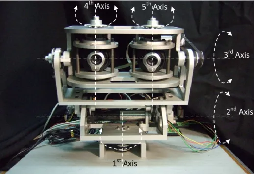
second axis. The binocular tilt-direction is set as the third axis, and the pan-directions of the cameras are set as fourth and fifth axes. Figure 3.3 defines axes of the five-axis Eye-robot. The Eye-robot head can rotate around a neck, but the neck was fixed in this research and only three degrees of freedom were used. The range of pan is approximately 120 degrees, and tilt is approximately 60 degrees. The size of the head is about 25 cm width and 10 cm height for the eye part.
As the purpose of the active vision system is to mimic the human system, the requirements of movement are also defined by human eye motion speed. The motor system is designed to achieve three 120 degree pan saccades per second and three 60 degree tilt saccades per second.
All motors are controlled which is attached to the host PC via the RS-232 interface card. The control and image process are both implemented in personal desktop computer with 1.60GHz CPU.
20
3.3 Software
The software for controlling the vision head of the Eye-robot, including capturing video, processing video image frames, and sending control signals for motor control, is written in MATLAB.
MATLAB is a high-level technical computing language and interactive environment for algorithm development, data visualization, data analysis, and numeric computation. Using the MATLAB product, we can solve technical computing problems faster than with traditional programming languages, such as C, C++, and Fortran.
In this thesis, the software of the MATLAB in a wide range of applications, including signal and image processing, communications, control design, test and measurement, financial modeling and analysis, and computational biology. Add-on toolboxes (collections of special-purpose MATLAB functions, available separately)
Figure 3.3 Definition of axes of the Eye-robot 1st Axis
2nd Axis 3rd Axis 5th Axis
21
extend the MATLAB environment to solve particular classes of problems in these application areas.
MATLAB provides a number of features for documenting and sharing the work. We also can integrate MATLAB code with other languages and applications, and distribute MATLAB algorithms and applications. Using MATLAB Features include: High-level language for technical computing
Development environment for managing code, files, and data
Interactive tools for iterative exploration, design, and problem solving
Mathematical functions for linear algebra, statistics, Fourier analysis, filtering, optimization, and numerical integration
2-D and 3-D graphics functions for visualizing data Tools for building custom graphical user interfaces
In this thesis, the software for controlling the vision head of the Eye-robot, include capturing image, processing image frames and sending control signals to each axis motors control which is written by M-file editor of Matlab R2006a. This is a kind of multitasking version of M-file editor produced in Matlab. All source code is written on the host PC desktop and compiled. The communication between PC desktop and Eye-robot are using RS232 to transmission signal from pc desktop to the Eye-robot controller. It handles Eye-robot tracking and sends the tracking status and coordinates of the object in the plane to pc desktop.
22
Chapter 4
Intelligent Object Tracking
Controller Design
In this chapter, the intelligent object tracking controller design applied to the Eye-robot will be introduced, including object detection and tracking controller design.
4.1
Object Detection
Recently, the image processing has been widely applied to lots of researches by transforming images into other forms of images, called the feature images, to provide useful information for problems in military, medical science, industry, etc.
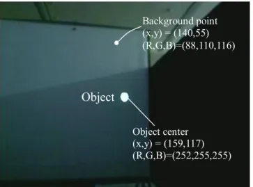
For simplicity, the object to be traced in this thesis is created by computer image which contains a white ball moving on a pure background in black and is projected on a screen, 240cm away from the Eye-robot. Figure 4.2 shows an image retrieved by the left-eye camera mounted on the Eye-robot. Clearly, in addition to the white ball and black background on the screen, there also includes undesirable things outside the screen in the image. To properly detect the white ball moving on the screen, this section will introduce some basic concepts and methods of image processing.
The pixels of the image retrieved by the Eye-robot are represented by a point (R,G,B) in the color cube as shown in Figure 4.1, where three axes are related to red, green and blue. Let the pixel be located at (x,y) with color (R,G,B), then its gray level can be expressed as
23
3 ,y R G B x Vgray (4.1-1)where 1x H and 1 y W. The values of H and W depend on the camera
resolution; for example, the image used in this thesis is of the size 320240, and thus
H=320 and W=240. Since the RGB space contains 256 levels, numbered from 0 to 255, along each axis in the color cube, there are 2563different colors in total and 256 different gray levels.
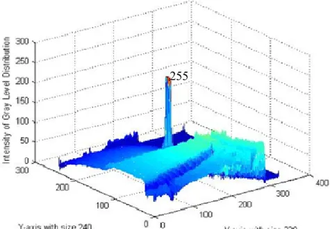
To detect the object on the screen, the image in RGB space of the left-eye camera in Figure 4.2 is first transformed by (4.1-1) into a gray level image as shown in Figure 4.3 with gray level intensity distribution given in Figure 4.4. Clearly, the gray level of the object, i.e., the white ball, is much higher than the other pixels and therefore a threshold can be easily selected for the object. Taking the threshold as 180 results in a binary image shown in Figure 4.5, where the pixel located at (x,y) is represented by black (0, 0, 0) blue (0, 0, 255) red (255, 0, 0) (255, 255, 255) white green (0, 255, 0) B R G
24
elsewhere y x V y x B gray 0 180 , 1 , (4.1-2)and Figure 4.6 shows gray level image distribution.
Based on this binary image, the location of the object in an image is detected and represented by the center (xc,yc) of the white region, which is B(x,y)=1. If there
are n pixels (xi,yi), i=1,2,…, n, in the region, then the object is located at center (xc,yc),
where n x x n i i c
1 (4.1-3) n y y n i i c
1 (4.1-4)After the object center (xc,yc) is obtained, the Eye-robot will be driven to trace the
object via offline training with the use of neural network, which will be introduced in the next section.
25
Figure 4.3 Image transform to gray level
Object center (x,y) = (159,117) Gray level=254 Object Background point (x,y) = (140,55) Gray level=105 Object center (x,y) = (159,117) (R,G,B)=(252,255,255) Object Background point (x,y) = (140,55) (R,G,B)=(88,110,116)
26
Figure 4.5 Binary image of taking the threshold as 180 Figure 4.4 Intensity of gray level distribution
27
4.2 Tracking Controller Design
This section describes the design of tracking controller, a neural-network-based controller, which is achieved via offline training. The input of the neural network is the object center p and the output is set to be the tracking index V related to the voltage needed to drive the Eye-robot. Figure 4.7 shows the feedback configuration of the tracking control, where the neural network controller receives the error e between the current horizontal position xc and the desired position xd of the
target and provides correspondingly a tracking index V to drive the Eye-robot. In this section, the neural network controller will emphasize with the training pattern that in used to drive the Eye-robot to trace the object.
Figure 4.6 Gray level image distribution
Object center (x,y) = (159,117) Gray level=255 Object Background point (x,y) = (140,55) Gray level=0
28
Figure 4.8 Eye training patterns 1 0.5 0.4 0.6 0.51 0.49 1 0 1 Tracking index (V1) Position (p1) Horizontal Position Detection Eye-robot Neural Network Controller V
Figure 4.7 Feedback configuration of the tracking
e Image xc Velocity Command xd ╳
Figure 4.9 Neck training patterns
Position (p2) 1 0.5 0.51 0.49 1 0 1 Tracking index (V2) 0.1 0.9
29
Now, let’s focus on the offline training of the neural network controller. There are two kinds of training patterns V1 and V2 used in this thesis and shown in Figure 4.8 and Figure 4.9. Note that the pattern V1 is expressed as
elsewhere p p p p V 0 6 . 0 0.51 09 . 0 51 . 0 0.49 0.4 09 . 0 49 . 0 1 1 1 1 1 (4.2-1)which is designed for the motion of the right eye or left eye. The pattern V2 is expressed as
1 0.9 1 9 . 0 0.51 39 . 0 51 . 0 51 . 0 0.49 0 0.49 0.1 39 . 0 49 . 0 1 . 0 0 1 2 2 2 2 2 2 2 2 p p p p p p p V (4.2-2)which is assigned for the motion of the neck. With these two patterns, the human visual motion can be mimicked. The left eye is selected as the dominant eye in this thesis and is designed to have the ability to find the object in searching mode. Once the object is detected, the eyes and the neck will work together to trace the object. Based on the training patterns, there are three kinds of the training modes for the Eye-robot. The first mode adopts three neural networks, including NNneck and two NNeye, for the neck, right eye and left eye, respectively. The neural network NNneck is trained by V2, while the neural networks NNeye are trained by V1. The second mode adopts two neural networks, including NNeye and NNeye1-neck, where NNeye is trained by V1, for the right eye and NNeye1-neck is trained by V1 and V2 for the dominant eye and the neck. The final mode employs only one neural network NNeye2-neck which is trained by V1, V1 and V2 for the right eye, the left eye and the neck simultaneously.
It is clear that the tracking motion is mainly executed by the neck when the object appears at the position far away the vision center xc, while the dominant eye
30
and right eye play the roles of concentration on the object. Based on the training patterns, when the object position p1 and p2 are located between 0.49 and 0.51, the center area, both the values V1 and V2 vanish. That means the Eye-robot already detects the object and will focus on it. In such situation, the Eye-robot keeps still and is not necessary to make any motion. If the object position p1 and p2 are located outside the center area, from the patterns V1 and V2 , the positions of the two eyes will keep unchanged and the neck will track the object faster when the object is farer away the center area. In addition, if the object is located in p2<0.1 or p2>0.9, the neck will track the object in the highest speed.
There are four neural networks used in this thesis, including NNneck, NNeye, NNeye1-neck, and NNeye2-neck. Their structures are all three-layered, containing input layer, hidden layer and output layer, depicted in Figure 4.10 to Figure 4.13. The structure of NNneck adopts one input signal and one output signal. By using 19 hidden neurons, NNneck is trained by the pattern (p2, V2) in Figure 4.10. The neural networks of individual eye, NNeye, adopt one input signal, one output signal and 81 hidden neurons, which are trained by the pattern (p1, V1) in Figure 4.11. For the combined neural network NNeye1-neck, it uses one input signal, two output signals and 131 hidden neurons, which is trained by the pattern (p1, V1) for the left eye and the pattern (p2, V2) for the neck in Figure 4.12. For the integrated neural network NNeye2-neck, it uses two input signals, three output signals and 151 hidden neurons, which is trained by the pattern (p1, V1) for the two eyes and the pattern (p2, V2) for the neck in Figure 4.13. With these four neural networks, there are three types of tracking control, named as
C3NN, C2NN and C1NN. The first type C3NN is composed of three neural networks, NNneck
and two NNeye for the neck, left eye and right eye. The second type C2NN contains two
neural networks, NNeye and NNeye1-neck, where NNeye is used for the right eye and NNeye1-neck is used for the left eye and the neck to operate together. As for the third
31
type C1NN, it employed only one neural network NNeye2-neck, which operates the neck and the two eyes simultaneously. To compare with these three types of tracking control, the third one seems to be simpler than the other two types.
Hidden Layer Input Layer Output Layer pneck Vneck
32 Hidden Layer Input Layer Output Layer
Figure 4.12 Structure of left eye combine with neck neural network pleft-neck Vneck Vleft-eye Hidden Layer Input Layer Output Layer Figure 4.11 Structure of eye neural network peye
33
Based on the back-propagation algorithm in Chapter 2, the neural networks designed for the tracking control is off-line trained according to the patterns (p1,V1) and (p2,V2). With the well trained neural networks, the Eye-robot can keep the object around the visual center.
After the offline training of the neural networks, the training results will be applied to the Eye-robot tracking. The Eye-robot kinematics allows pan and tilt motion and then can trace any object moving left-and-right or up-and-down. The motion of the Eye-robot, with five degrees of freedom, is designed to keep the object at the center of the image retrieved by the Eye-robot. During the object tracking, each Eye-robot motor will get an appropriate tracking index depending on the object location via neural network off-line training. However, the tracking indeces are obtained under normalization and between 0 and 1, not available for driving the Eye-robot. Hence, the desired voltage input of each motor is determined by
Hidden Layer Input Layer Output Layer pleft-neck Vneck Vleft-eye
Figure 4.13 Structure of left eye combine with neck and right eye neural network Vright-eye pright
34
vinput Vvmax (4.2-3)
which multiplies the maximum voltage vmax to the index V . Obviously, the larger
the voltage input v, the faster the tracking speed of the Eye-robot.
In this thesis, the object tracking is fulfilled by the neck and two cameras simultaneously. When the object is found, the Eye-robot is driven by all the motors together to track and then focus on the object at the visual center. Figure 4.14 shows the block diagram of the Eye-robot visual tracking control design architecture.
35
Image Capture
Object Detection Threshold>180
Initialize system
Calculate Object Position
No
Yes
Neural Network Controller
Eye-robot
Figure 4.14 Block diagram of the Eye-robot visual tracking control design architecture RGB2Gray Level
Velocity Command p
36
Chapter 5
Experimental Results
This chapter shows the experimental results, including the neural network off-line training and the intelligent tracking control, to demonstrate the success of the multiaxial control designed for the Eye-robot.
5.1 Neural Network Off-line Training
This section focuses on the off-line training of the four neural networks, NNneck, NNeye, NNeye1-neck, and NNeye2-neck, used in the tracking controllers, C3NN, C2NN
and C1NN, introduced in Chapter 4. It is known that different types of tracking control
requires different types of neural networks. Besides, all the neural networks are designed to have three layers, the input layer, output layer and hidden layer. The number of neurons of the input layer is chosen to be the same as the number of input data, so is the number of neurons of the output layer, corresponding to the output data. However, how many neurons are needed for the hidden layer should be determined by experiments, via neural network off-line training in this thesis.
First, let’s find the suitable number of neurons of NNneck and NNeye, which will be applied to the controller C3NN. The off-line training of NNneck is executed in different cases, named as NNneck-k where k is the number of neurons of its hidden layer and is chosen from 10 to 30. Based on the off-line training, it can be found that the learning time is decreased sharply while k is changed from 18 to 19, as shown in Table 5.1. Obviously, the NNneck-19 is the best structure when comparing with others. Thus, the NNneck-19 will be used in the controller C3NN to control the neck. Similarly,
37
the best structure with minimal learning time and epochs. Hence, two of the NNeye-81 will be used in the controller C3NN to control the right eye and left eye.
Table 5.1 Neck neural network off-line training parameter
Experiments NNneck-10 NNneck-18 NNneck-19 NNneck-20 NNneck-30
Learning Time 71 66 21 25 48 Epochs 18381 12135 3589 4514 6564 Hidden neurons 10 18 19 20 30 Tolerance 10-3 10-3 10-3 10-3 10-3 Learning rate 0.01 0.01 0.01 0.01 0.01 Input neuron 1 1 1 1 1 Output neuron 1 1 1 1 1
Table 5.2 Eye neural network off-line training parameter
Experiments NNeye-60 NNeye-80 NNeye-81 NNeye-82 NNeye-100
Learning Time 5610 4317 1834 2399 5929 Epochs 138402 109820 50662 63851 125361 Hidden neuron 60 80 81 82 100 Tolerance 10-3 10-3 10-3 10-3 10-3 Learning rate 0.01 0.01 0.01 0.01 0.01 Input neuron 1 1 1 1 1 Output neuron 1 1 1 1 1
Next, let’s find the suitable number of hidden neurons of NNeye1-neck, which is applied to the controller C2NN. The off-line training of NNeye1-neck is also executed in different cases, named as NNeye1-neck-k where k is the number of neurons of its hidden layer and is chosen from 110 to 150. Based on the off-line training, it can be found that the learning time is decreased sharply while k is changed from 130 to 131 and then increased sharply while k is changed from 131 to 132, as shown in Table 5.3. Obviously, the NNeye1-neck-131 is the best structure when comparing with others. Thus, the NNeye1-neck-131 will be used in the controller C2NN to control both the left eye and
the neck simultaneously. Besides, the NNeye1-81 is also included in C2NN to control the
38
Table 5.3 Left eye combine with neck neural network off-line training parameter Experiments NNeye1-neck-110 NNeye1-neck-130 NNeye1-neck-131 NNeye1-neck-132 NNeye1-neck-150
Learning Time 4752 4188 2408 4726 5001 Epochs 112662 80353 42112 85029 88619 Hidden neuron 110 130 131 132 150 Tolerance 10-3 10-3 10-3 10-3 10-3 Learning rate 0.01 0.01 0.01 0.01 0.01 Input neuron 1 1 1 1 1 Output neuron 2 2 2 2 2
Finally, let’s find the suitable number of hidden neurons of NNeye2-neck, which is applied to the controller C1NN. Similarly, NNeye2-neck-k represents the case of the off-line training of NNeye2-neck with k neurons in the hidden layer chosen from 130 to 170. From Table 5.3, the NNeye2-neck-151 is the best structure when comparing with others. Besides, interestingly an abrupt change in learning time still exists around k=151, same as the other three neural networks mentioned previously. According to Table 5.3, the NNeye2-neck-151 will be used in the controller C1NN to control the neck
and both the two eyes at the same time.
Table 5.4 Left eye combine with neck and right eye neural network off-line training parameter
Experiments NNeye2-neck-130 NNeye2-neck-150 NNeye2-neck-151 NNeye2-neck-152 NNeye2-neck-170
Learning Time 6802 4036 3512 5547 6748 Epochs 169082 89044 77113 118173 137133 Hidden neuron 130 150 151 152 170 Tolerance 10-3 10-3 10-3 10-3 10-3 Learning rate 0.01 0.01 0.01 0.01 0.01 Input neuron 2 2 2 2 2 Output neuron 3 3 3 3 3
39
5.2 Set Point Control
This section will employ the neural networks well-trained by the back-propagation learning algorithm to drive the Eye-robot such that the object is traced, i.e., the object is kept in the image center. In the experiments, an image of a circle with radius 5cm projected on a screen is used as the object to be traced and the distance between the screen and the Eye-robot is 280cm. During the object tracking, the maximal velocity of the neck is set to be vmax=1500rpm/min. For an individual eye, not working together with the neck, its maximal velocity is set to be 70 rpm/min. However, when an eye works together with the neck, its maximal velocity is not necessary to be 70 rpm/min, but is lowered down to 30 rpm/min.
Figure 5.1 to Figure 5.3 show the results of the C3NN set-point control of an
fixed object whose image is initially located at the position left to the visual center. The controller C3NN contains three neural networks, NNneck and two NNeye. Figure 5.1 shows the tracking index produced by NNneck and the position error of the object to the visual center. Obviously, with the tracking index the motor mounted to drive the neck has successfully reduced the position error. From Figure 5.2 and Figure 5.3, it is clear that the motors employed to steer the two cameras have also reached the control goal to locate the object around the visual center with an error near to zero.
40
Figure 5.2 Set-point control of NNeye results of the right eye
41
Figure 5.4 and Figure 5.5 show the results of the C2NN set-point control under
the same conditions. There are two neural networks, NNeye1-neck and NNeye, to implement the controller C2NN. Figure 5.4 shows the tracking indices produced by NNeye1-neck for the left eye and the neck. With the tracking indices the position error has been reduced to zero as expected. For Figure 5.5, the motor employed to steer the right eye has also successfully located the object around the visual center with an error near to zero.
42
Figure 5.5 Set-point control of NNeye results of the right eye
Figure 5.4 Set-point control of NNeye1-neck results of the left eye combine with neck
43
Finally, Figure 5.6 shows the results of the C1NN set-point control which uses
only one neural network NNeye2-neck to control the neck and two cameras simultaneously. In this figure, both the position errors related to the two eyes have been reduced to zero by the three tracking indices generated by NNeye2-neck.
Once the object is detected, the two eyes and the neck will work together to trace the object. Whatever the place of the object location, it is clear that the Eye-robot will detect the object then trace the object in the center within 2 seconds and maintain the object in the center. These experimental results will be performed to demonstrate the effectiveness of the proposed scheme.
To demonstrate that the controllers C3NN, C2NN and C1NN are also suitable for the set-point control of a fixed object initially located right to the visual center, Figure 5.7 to Figure 5.9 show the experiment results of the image position errors related to the two eyes. In these figures, it is clear that the controllers C3NN, C2NN and C1NN indeed successfully drive the object image to the visual center.
Figure 5.6 Set-point control of NNeye2-neck results of the left eye combine with neck and right eye
44
Figure 5.8 Set-point control of C2NN errors result Figure 5.7 Set-point control of C3NN errors result
45
5.3 Horizontal Object Tracking Control
This section will further focus on the tracking control of horizontal trajectories and similar to set-point control the maximal velocities are set to be vmax=2000rpm/min for the neck, 70 rpm/min for the individual eye and 30 rpm/min for the eye to work with the neck. The horizontal trajectory is sinusoidal and expressed as
) 2 cos( ) ( T t A t x (5.3-1)
where A is the magnitude and T is the period. In the experiments, A=70 and the T= 6, 9, 12, 15 seconds. For the case of T=6 seconds, the experiment results of the image position errors are shown in Figure 5.10 to Figure 5.12. From these results, it is clear that all the controllers C3NN, C2NN and C1NN are indeed able to control the Eye-robot to trace the moving object with image position errors less than 0.09, i.e., within 30 pixels. Such image position errors are acceptable since the radius of the object, which is 6
46
pixels with the tracking errors around 0.02, and results in a quite smooth tracking
motion.
47
Figure 5.12 6 seconds of C1NN errors tracking control result Figure 5.11 6 seconds of C2NN errors tracking control result
48
Intuitively, a slower moving object will lead to a more precise tracking motion. To demonstrate such tracking behavior, the controllers C3NN, C2NN and C1NN are also applied to the cases of T=9,12,15 seconds. Figure 5.13 to Figure 5.15 show the experiment results for T=9 seconds, Figure 5.16 to Figure 5.18 show the experiment results for T=12 seconds, and Figure 5.19 to Figure 5.21 show the experiment results for T=15 seconds. As expected, the image position errors are reduced to 20 pixels for T=9 seconds and to 15 pixels T=12 seconds. However, limited to the physical feature of cameras, the image position errors are no longer improvable by further decreasing the period to T=15 seconds, whose image position error is still around 15 pixels.
In experiment results have been conducted in conditions and the experimental results have proved that the Eye-robot tracking in an effective for accurately and rapidly tracking moving object. Obviously, when the object is far away to the image center, the highest velocity will be obtain in object tracking control, the left eye with the neck and the right eye of the Eye-robot can trace the object in the center by smoothing and quickly simultaneously. To demonstrate the proposed, both computers and experiments are executed in this thesis. During the experiment results, different cases are executed to evaluate the feasibility for the proposed scheme. In these experiment results, the results show that the proposed has excellent performance to achieve the Eye-robot tracking
49
Figure 5.14 9 seconds of C2NN errors tracking control result Figure 5.13 9 seconds of C3NN errors tracking control result
50
Figure 5.16 12 seconds of C3NN errors tracking control result Figure 5.15 9 seconds of C1NN errors tracking control result
51
Figure 5.18 12 seconds of C1NN errors tracking control result Figure 5.17 12 seconds of C2NN errors tracking control result
52
Figure 5.20 15 seconds of C2NN errors tracking control result Figure 5.19 15 seconds of C3NN errors tracking control result
53
54
Chapter 6
Conclusions and Future Works
This thesis proposes an intelligent object tracking controller design to drive the Eye-robot to trace the object and the object detection method to fix with the image. The proposed of the Eye-robot tracking in this thesis has shown that it is possible to use a neural network controller to compute actual velocity with good accuracy. This thesis used an ANN to train the training patterns such that, when the object is presently located in any places, it automatically computes the velocity V of the corresponding object position p. The Eye-robot tracking controller design that is used in this thesis is very simple in concept, independent of the Eye-robot model used and the quality of image obtained and yields very good results.
The experimental results in the thesis show that an acceptable accuracy can be obtained but it seems that is not very easy to reach high accuracy by using only neural networks. Neural networks have a good generalization capability in the range that they are trained. During the object tracking, the image capture, image processing and to give a velocity command to drive the Eye-robot only spent around 0.15 second.
The Eye-robot was successful applied in the object tracking, which via the offline training with the use of neural network. For the future studies, there are some suggestions and directions described as follows:
1. Extend to five-axis motors, which is increase vertical direction to track the motion object.
2. Track a designated object in multiple objects even when they are moving together, or interacting with each other.