玻色愛因斯坦凝聚於光晶格中靠近零色散點的行為

國立交通大學

物理研究所

碩 士 論 文

The behavior of BEC in optical lattices

near the zero-dispersion point

研究生：陳慶憲

指導教授：江進福 教授

The behavior of BEC in optical lattices

near the zero-dispersion point

研 究 生：陳慶憲

Student：Ching-Hsien Chen

指導教授：江進福 教授

Advisor：Tsin-Fu Jiang

國 立 交 通 大 學

物 理 研 究 所

碩 士 論 文

A Thesis

Submitted to Institute of Physics

College of Science

National Chiao Tung University

in partial Fulfillment of the Requirements

for the Degree of

Master

in

Physics

June 2005

Hsinchu, Taiwan, Republic of China

玻色-愛因斯坦凝聚態於光晶格中

靠近零色散點的行為

研究生：陳慶憲 指導老師：江進福 教授

國立交通大學物理研究所

摘要

我們使用一個方法去探討玻色-愛因斯坦凝聚態在光晶格中靠近零色散點 附近的行為。玻色-愛因斯坦凝聚態可由一維的 Gross-Pitaevski 方程式來描述其 動力學行為，並且可以應用等效質量法將之以非線性薛丁格方程來描述。當考 慮零色散點附近的行為時即第二階色散效應趨近於零,必須考慮第三階的色散 效應。此時玻色-愛因斯坦凝聚態將由廣義的非線性薛丁格方程來描述，我們利 用由逆散射法之非線性薛丁格方程的解在小振幅的限制下找出一個假設解解出 廣義的非線性薛丁格方程(即考慮第三階色散效應)之進似解析解，我們得到一 個可以存在大部份區域之暗孤子以及在一個特殊區域時暗孤子將轉成光孤粒子 的解,即所謂的在背景上的孤立子。此外，我們利用直接的模擬數數值解來觀察 其解析解的存在性。同時,在數值解我們可以觀察到當在較大的振幅時將產生一 個輻射衰退的效應,此效應被認為是由於第三階色散的影響。

i

The behavior of BEC in optical lattices

near the zero-dispersion point

Student: Ching-Hsien Chen Advisor: Prof. Tsin-Fu Jiang

Institute of Physics

National Chiao Tung University

Abstract

We demonstrate a method to analytically study the effective-mass method of Bose-Einstein Condensates (BEC) in optical lattices near the zero dispersion (Z-D) point where the effect of the second-order dispersion is zero. We use one dimensional Gross-Pitaevskii (G-P) equation describes the dynamic behavior of BEC to the optical lattices. By using effective-mass theory to our system in the neighborhood of the Z-D point we need to consider the third-order dispersion term to our equation. That is, our system is described by the generalized NLS equation. We take the dark-soliton solution form of the NLS equation solved by inverse scattering method in the small amplitude limit as an assumed solution to substitute into our equation. We obtain dark solitons solution may exist near the Z-D point and we also show a region near the Z-D point where a special solitary wave form, the so-called soliton on the constant background, may be observed. We use directly numerical simulations of the full generalized NLS equation which includes the third-order dispersion term to observe that the existence of the new solitary wave form. Numerical computation also shows that a radiation emission exits near the Z-D point in the larger amplitude, which is regarded as the effect of three-order dispersion

誌 謝

對於即將要畢業的我來說，有著許多的感觸。想當初兩年前剛入學時的懵 懂無知到如今即將完成此本碩士論文的我，這兩年的碩士生涯著實地讓我有許多 的成長。這一切都要感謝許多人，他們熱心的指導和討論無論是在課業上或是在 生活上。首先我要感謝我的指導老師江進福教授，提供一個好的環境讓我們可以 自由的發揮和研究，並且也提供許多的建議和幫助給我，當我遇到困難時。我同 時也要感謝中國文化大學物理系的程思誠教授，他的許多建議和熱心的指導讓我 常能順利地解決許多我苦思已久的問題，使我順利地完成研究。 感謝我的夥伴們，華潔、政果和瓊瑩，給我的許多幫助和討論。我想不管以 後往那裡走，我都會懷念這段碩士時光的，和大家相處的時光。還有葛威成、官 文绚學姐和柯藝謀學長也提供許多他們寶貴的經驗和想法給我，無論在學術研究 上或是學習上。在此，我也非常感謝他們。 最後，要感謝我的家人爸、媽、弟弟和妹妹對我的支持與關心! 尤其是我的 父母，我想致上我無盡的感激。他們全心全力無條件地支持我，讓我能毫無顧忌 地專心學習在學業上。

民國九十四年六月

iii

Content

Abstract (in Chinese) ...………….……….…….……. i

Abstract (in English) ...………….……….…...………ii

Acknowledgement (in Chinese) …………..……….……...……iii

Content ..……….……….….….…...iv

List of Figures ……….….…….…..vi

Chapter 1 Introduction

……….…...1

1-1 Preface ……….……….……...….1

1-2 Motivation………...……3

1-3 Organization of this Thesis ……….….……….……....….4

Chapter 2 Theory and Methodology

………..……….……...…...5

2-1 Bose-Einstein condensates in optical lattices ...5

2-1-1 Effective Mass method in Bose-Einstein condensates…...7

2-1-2 Band structure…...9

2-2 The method for solving generalized NLS equation...13

2-2-1 The solution of NLS equation in the small amplitude regime...13

2-2-2 The solution of generalized NLS equation in the small

amplitude regime……... 15

Chapter 3 Numerical simulation

……….……...…25

3-1 Numerical method…...25

iv

3-1-1 Numerical simulation of the generalized NLS equation...28

3-2 Numerical simulation of BEC in optical lattices near the

zero dispersion point……...34

Chapter 4 Conclusion and perspective

…….….….…..….…..42

References

…………...………….….…..….……43

List of Figures

Fig. 1 The time evolution with the arbitrary coefficients where µ =0.3…….……….30 Fig. 2 The time evolution with the arbitrary coefficients whereµ =0.3,

but the third-order dispersion term is absent………...…………31

Fig. 3 The time evolution of a special initial profile which subtracts the background from the initial profile of fig. 1 with the same conditions……….………32 Fig. 4 The time evolution of a special initial profile which subtracts the background

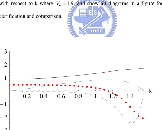
from the initial profile of fig. 2 with the same conditions…….………33 Fig. 5 The initial conditions is same with fig. 1 whereµ =0.5...33 Fig. 6 The derivatives of band structure with respect to k………..34 Fig. 7 Second and the third derivatives of band structure with respect to k

in comparison with nonlinear coefficient………. ….………..35

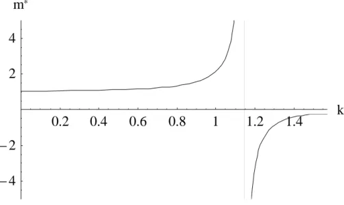
Fig. 8 The plot of effective mass with respect to k……….………..36 Fig. 9 The time evolution of anti-dark soliton where k=0.8 and µ =0.3….…………37 Fig. 10 The time evolution of anti-dark solliton where k = 0.8 and µ =0.5.….………38 Fig. 11 The plot of δ with respect to k………38 Fig. 12 The time evolution of a special initial profile which subtracts the background from

the initial profile of fig. 6 with the same condition.………39 Fig. 13 The time evolution of a special initial profile which subtracts the background

from the initial profile of fig. 7 with the same condition.……….………40 Fig. 14 Choosing a Gaussian initial profile to plot the time evolution of BEC

in the anomalous regim….………….………40

Chapter 1 Introduction

1-1 Preface

The basic idea of Bose-Einstein condensation (BEC) dates back to 1925 when A. Einstein devoted to the statistical description of the quanta of light and predicted the occurrence of a phase transition in a gas of non-interacting atoms on the basis of a paper by Indian physicist S.N. Bose (1924). This phase transition is associated with the condensation of atoms in the state of lowest energy and is the consequence of quantum statistical effects. For a long time this predictions had no practical confirmation until the experimental cooling technique had been advanced to the lower temperature [1].

Bose-Einstein condensation was observed in a remarkable series of experiments since 1995 on the vapors of rubidium (Anderson et al., 1995) and sodium (Davis et al., 1995) in which the atom were confined in magnetic traps and cooled down to the extremely low temperature, of the order of fractions of micro-kelvins. The first evidence for condensation emerged from time-of-flight measurement. The atoms were left to expand by switching off the confining trap and then imaged with optical methods [2]. Afterward, the successful experimental achievement to BEC had grown more fast as if a blast in the recent 10 years.

At low enough temperature the condensate evolution is described sufficiently well by the Gross-Pitaevskii (G-P) equation [2], which is originally three dimensional (3D) but in the case of a cigar-shaped trap potential it is reducible to a 1D nonlinear Schrödinger (NLS). Its validity is based on the condition that s-wave scattering length

be much smaller than the average distance between atoms and that number of atoms in the condensate be much larger than 1 . Under this condition , our system which is BEC in optical lattices can be simplified as the nonlinear Schrödinger equation with periodic potentials. As the numerous experiments of BEC had been observed , many physical properties of BEC might be predicted and investigated to understand the fabulous phenomenon of BEC advanced . For example : first experimentally loading BECs in optical lattices [3] , subsequently lattice effect has attracted considerable attention, Bloch oscillations [4], superfliud and dissipative dynamics[5] , dispersion[6] and Landau-Zener tunneling[7] and so on

BEC in optical lattices are affected by the structures of optical lattices. The BEC spectrum has an associated band structure .If the atomic density is high, BEC behaves nonlinearly. As the nonlinear term exactly compensates for dispersion term, solitons occur. The properties of the atoms are characterized by the depth and period of this optically induced potential. If the potentials happen to be deep enough, and only consider the first band, these self-localized states are known as discrete solitons simply because they can be described by the tight-binding approximation. As for the relatively shallow potentials, when the eigenvalue is located in the gap between two successive bands, these self-localized states are known as gap solitons[8] and are described by coupled mode approximation which we only consider two successive bands in the lowest two bands[9].

1-2 Motivation

The gap solitons of atoms has been observed experimentally in the BEC with the repulsive atom-atom interaction [10] to show that effective-mass analysis does allow us to describe the behavior of BEC. With the effective mass analysis of BEC in optical lattices one can obtain a 1D nonlinear Schrödinger (NLS) equation deduced from the G-P equation without the need for full-scale numerical calculations. In this thesis the periodic potentials ,which are optical lattices, are assumed to be relatively shallow potential which can be correctly described by the coupled mode theory. It’s well known that the atoms confined to infinite periodic potential behave as if it possessing an effective mass which is substantially different from its true mass, and may even be taken a negative mass [11]. Our interest is near the regimes of the turning point of the band structure, which the so-called Zero dispersion point in the optical fiber, that the effective-mass approaches infinity and the coefficient of second-order dispersion term is almost zero. One can assume that one has to include the third-order dispersion to the equation which nonlinear Schrödinger equation becomes the generalized nonlinear Schrödinger equation. Nonlinear Schrödinger equation is studied thoroughly and exactly solved by the inverse scattering method, contrary to the exactly analytical solutions of the generalized nonlinear Schrödinger equation are not available, and the equation is non-integrable by inverse scattering method. In this thesis we mainly study the properties of this equation solved by an assumed solution based on the exact solution of nonlinear Schrödinger equation solved by inverse scattering method in the small amplitude limit to predict the possible behaviors of the atoms in the optical lattices. As for the numerical simulations, we deal with the full generalized nonlinear Schrödinger equation which includes the third-order dispersion term to give some confirmation about our analysis

due to our analytic solution which is an lowest-order approximated solution solve by perturbation method .

1-3 Organization of the Thesis

This Thesis is organized as follows. Chapter 2 gives a brief review about the effective-mass analysis of BEC in optical lattices to derive the equation which we are interested from G-P equation. Then, we describe our method in detail to analytically solve the generalized nonlinear Schrödinger equation. In the chapter 3 we look for some numerical evidence to give our analysis some confirmation and observe some possible behaviors of BEC in the optical lattices near the zero-dispersion point by numerical simulation. Then, in the chapter 4, the last chapter, we briefly conclude our results that we obtain from both theoretical and numerical analysis.

Chapter 2 Theory and methodology

G-P equation is the main theoretical tool for investigating non-uniform dilute Bose gases at low temperature that it can well approximately describe the dynamic behavior of BEC. With the effective-mass analysis of BEC in optical lattices and assuming the optical lattices are shallow periodic potential one can simplify the G-P equation to a much simply equation which is the nonlinear Schrödinger equation in one dimension . The use of this approach has been confirmed by the BEC experiment of gap soliton [10]. In this thesis we discuss the regimes near the zero-dispersion point where the nonlinear Schrödinger equation has to be included the third-order dispersion term which we usually ignore it. The generalized nonlinear Schrödinger equation has no exactly analytic solution at present. We demonstrate an method to approximately analyze the properties of the atoms near the zero-dispersion point that the method bases on an exactly analytic solution of NLS equation in a small amplitude limit by inverse scattering method as an assumed solution to substitute into the generalized non-linear Schrödinger equation.

2-1 Bose-Einstein condensates in optical lattices

The dynamics of a Bose-Einstein condensate in an optical lattice can be

described by the Gross-Pitaevskii (GP) equation [2],

2 2 2 ( , ) ( ) ( ) ( , ) 2 as t i V x U g t m ψ ⎡ ⎤ ∂Ψ ₌ − _{∇ + + + Ψ} ⎢ ⎥ ∂ _{⎢⎣ ⎥⎦} r r r t (2.1)

where is Planck’s constant, is the mass of the atoms, is the nonlinear coefficient, and

m 4 2/

s

a s

g = πa m

s

a is the s-wave scattering length. is a one-dimensional periodic potential produced by the interference of laser beams, where

2

( ) _osin ( / ) V x =E πx L

L is the lattice constant and is the potential depth. o E 2 2 2 2 2 1 ( ) ( ) 2 r _x

U = m⎡_⎣ω x +ω_⊥ y +z ⎤_⎦ is an optical trapping potential with frequencies ω_x and ω_⊥. The trap is elongated along the x direction because of the high confinement in the y-z plane (i.e.ω_x ω_⊥). Therefore, we assume the wave function as Ψ( ; )r t =a y z( , ) ( , )ψ x t , where the two-dimensional harmonic oscillator problem,

( , )

a y z

2 2 2 2 2

(− / 2 )m ∇_⊥a+(mω_⊥/ 2)(y +z )a= Ω_⊥a. By applying the transformation exp(ψ →ψ − Ωi _⊥t)and integrating Eq.(2.1) with respect to y, z. then a one-dimensional G-P equation is derived as

2 2 2 2 2 ( , ) sin ( ) ( , ) 2 2 s a o g x t i E x t m _x L ψ ⎡ π _ψ ⎤_ψ ∂ ₌ − ∂ _{+ +} ⎢ ⎥ ∂ _{⎢⎣ ∂ ⎥⎦} x t . (2.2)

by rescalingT =t T/ _o,X =x L/( / 2),ψ ϕ= / L1/ 2₁ , and V_o =E_o/ε₀, and choosing ,

2_{/ 4}

o

T =mL L₁=ω_⊥ a mL_s 2/ 2 , and . Here, we had dropped the trap of z-axis. Then, an effective one-dimensional G-P equation with dimensionless is derived as 2 0 4 / mL ε = 2 2 2 2 2 ( , ) 1 sin ( , ) 2 o 2 X T i V X T _X ϕ ⎡ π _{σ ϕ ϕ}⎤ ∂ _=⎢− ∂ ₊ ⎛ ⎞_{+ ⎥} ⎜ ⎟ ∂ _{⎢⎣ ∂ ⎝ ⎠ ⎥⎦} X T , (2.3)

whereσ = sgn a( _s), Eq.(2.3) is a time-dependent nonlinear Schrödinger equation with a periodic potential. If σ is positive (negative), atoms are in repulsive

(attractive) interaction.

2

N =

∫

_−∞∞ ϕ dX , (2.4)

which means the conservation of the number N of atoms in the condensate.

2-1-1 Effective-mass method in Bose-Einstein condensates

Effective mass method is a well-known in solid state physics for studying dynamics of an electron in semiconductor. The two systems between electrons in semiconductor and BEC in optical lattices are analogue that we can introduce the effective mass theory to study BEC in optical lattices [12]. Expanding the condensates wave function ϕ( , )X T on the complete set of Bloch functionφ_nκ( )X , which

( )

(

,

)

,

(

, )

_n

(

, )

_n

exp

_n n

X T

A

_κ

X T

_κ

X

iE

T

κ

ϕ

=

∑

φ

−

_{κ . It is motivated that the}

Bloch functions can capture the rapid oscillation of the condensates wave function, then the slow essential motion of the condensate will be described by the slowly varying envelope function .To construct the localized state we assume that the matter wave field is characterized by a central wave vector

n

A_κ

0

κ corresponding to the mean velocity of the condensate. We expand ϕ( , )X T as

(

)

0 , 0 ( , ) _n ( , ) _n ( ) ex p _n n X T f _κ X T _κ X iE _κ

ϕ

=

∑

φ

− T (2.5)

(

0

)

0

( , )

( )

i X

n n

f

_κ

X T

=

∫

A

_κ

T e

κ κ−

d

κ

From eq.(2.5) , we have

(

)

0 ,

(

, )

_n

( )

_n

(

) exp

_n n

X T

A

_κ

T

_κ

X

iE

_κ

T d

0

ϕ

=

∑ ∫

χ

−

κ

_(2.6) Where

(

0

)

0

(

)

i X

(

)

i X

(

)

n

X

e

n

X

e

n κ κ κ κ κ

χ

=

−

φ

=

φ

_κ

X

and 0 2 ( ) 1 nκ X d X

φ

=

∫

Inserting eq.(2.6) into eq.(2.3) and applying effective-mass method , at last performing an inverse Fourier transform from A_nκ( )T back to

0( , ) n f _κ X T . Then, we obtain 0 0 0 0 2 3 3 ₂ 0 _{* 3}

( , )

( )

1

( )

( , )

( , )

6

2

n n n g n n

f

X T

p

v p

p

g f

X T

f

X T

i

T

m

κ κ κ κ

ε κ

ε κ

σ

κ

∧ ∧ ∧

⎡

⎤

∂

⎢

₊

₊

₊

∂

₊

⎥

₌

⎢

⎥

_∂

∂

⎢

⎥

⎣

⎦

(2.7) where 0

( )

n g

v

κ

ε κ

κ

∂

=

∂

, 0 2 * 2

( )

1

_n

m

_κ

ε κ

κ

∂

=

∂

, and 0

4

( )

n

g

=

∫

φ

_κ

X

dX

replacing p ∧

by its configuration space representation i

X ∂ − ∂ to eq.(2.7) 0 0 0 0 0 0 2 3 2 0 * 2 3

1

( , )

( )

2

n n n n g n

f

f

f

f

i

iv

i

g f

X T

f

f

T

X

_m

_X

_X

κ κ κ κ 0 n n n κ κ κ

η

σ

ε κ

∂

∂

∂

∂

+

=−

+

+

+

∂

∂

_∂

_∂

(2.8)

where 0 3 3

( )

1

6

n κ

ε κ

η

κ

∂

=

∂

, and σ = sgn a( _s). Whenσ = − , the nonlinear 1 term is attractive interaction. On the contrary, asσ = , the nonlinear term is repulsive 1 interaction.

2-1-2 Band Structure of BEC in optical lattices

To study BEC in optical lattices which is a series of periodic potentials we are to look for the past fundamental theory based on the solid state physics. With the help of the solid state physics we can describe the atomic matter waves in E-k band structure which is the similar manner that we study the properties of electron under linear Schrödinger equation. To find the band structure we assume that the linear part of Eq. (2.3) has stationary solutions of the formϕ( , )X T =ν(X) exp(−iET). we thus obtain the following eigen-value problem

2 2 2 1 ( ) sin ( ) 2 o 2 X E X V X X π ⎡_{− ∂ ⎛ ⎞}⎤ Ψ =⎢ + _{⎜ ⎟} Ψ ⎝ ⎠ ∂ ⎢ ⎥ ⎣ ⎦⎥ (2.9)

Eq. (2.5) has periodic solutions which are known as Floquet-Bloch (FB) modes [9]. By using plane-wave methods, the periodic potential can be expanded as

sin (2 / 2)

(

)

2 4 i X i X o o o V V V πX = − eπ +e−π (2.10) And the Bloch functions can be expressed as _{n k,} ( ) _{n k,} ( ) _m im X

m

So we expand ( ) ( , ) _m i k m X m X k b e + π Ψ =

∑

(2.11)

and satisfy orthonormality. Substituting Eq. (2.11) into Eq. (2.10) , we have

(

2

(

)

2

)

_{1 1} 0 2 2 o o o m m m V V E V− − k+mπ b + b ₋ + b ₊ = (2.12)

This method can be accurate as long as we consider the number of plane wave expansion large enough. We assume the potential is relatively shallow, and the bands between the first and the second band can be accurately described by keeping only two terms of the expansion, i.e.m= −0, 1 _{,which we assume the coupling of two band.} Eq. (2.11) is rewritten as

φ

( , )X k =b e_o ikX +b e₋₁ ikXe−i Xπ (2.13) Then, we obtain the following coupled equations

(

)

2 1 2 1 1 2 2 4 2 2 2 o o o o o o o V k V E b b b k V V E b b π − b − − ⎧⎛ ₋ ⎞ _{= −} ⎪⎜ ⎟ ⎪⎝ ⎠ ⎨ − ⎛ ⎞ ⎪ _{− = − +} ⎜ ⎟ ⎪⎝ ⎠ ⎩ (2.14)

(

)

2 0 2 1 2 2 4 0 2 2 2 o o o o V k V E b b k V V E π − ⎡ ⎤ − − ⎢ _{⎥ ⎛ ⎞} ⎢ ⎥_{⎜ ⎟=} ⎢ _{− ⎥ ⎝ ⎠} ⎢ _{− −} ⎥ ⎢ ⎥ ⎣ ⎦ (2.15)

With the ortho-normal condition of the Bloch functions we obtain

( )

(

)

1 2 2 2 0 1 1 2 x dx b b₋ − Ψ = +

∫

=1 (2.16) By solving the system of linear equations Eq.(2.15) E-k band structure of one-dimensional BEC in optical lattices is then derived as

2 2 2 2 _{( )}2 _{( ( ) )} 2 4 4 o o k k V V k k E = + + −π ± − −π + 2 (2.17)

where the wave-vector k is −π 2≤ ≤k π 2 _{in the first Brillouin zone. Substituting} the solution of the lowest band which that we choose the minus sign in Eq. (2.18) into the system of linear equations Eq.(2.15) , we obtain a set of nontrivial solution that it is essentially important in computing the coefficientg , but here instead of directly solving the system of linear equations we make use of the orthonormal condition to deduce the coefficientg . So we obtain

0 4 _{2 4} 0

1

( )

2

4

2

n

g

=

∫

φ

_κ

X

dX

= −

b

+

b

_{0 (2.18)}

where

(

)

(

)

(

)

1 2 2 2 2 2 2 2 2 0 0 0 2 2 2 0 b V V π π k π π k π π k V − ⎡ ⎤ = _⎢ + − − − − + _⎥ ⎣ ⎦ , with the

determination of specific and we can obtain the coefficient of nonlinear interaction

k V₀

gfrom . As for the other coefficients, they also has been decided once we

determine the specific k and V₀, they are described as follows :

0

( )

g

v

κ

ε κ

κ

∂

=

∂

, 0 2 * 2

( )

1

_n

m

_κ

ε κ

κ

∂

=

∂

, ε κn( 0).

2-2 The method for solving generalized NLS equation

In the following, we will use a method for solving the generalized NLS equation in question which has been demonstrated by Kivshar in the optical fiber [12] , [13] that the equation of optical fiber has the analogue with the equation of BEC in question, and it had been investigated for several decades in the optical fiber. This method is based on the solution, of dark soliton case, of NLS equation solving by inverse scattering method in the small density regime that we assume a similar solution form to substitute it into the generalized NLS equation we are interesting. Then, by applying the technique of nonlinear analysis we can obtain a connection between the nonlinear Schrödinger and the Korteweg-de Vries (Kdv) equations. Since we can solve Kdv equation by directly integrating, we can obtain the solution of the NLS equation with the third-order dispersion term in the small amplitude regime.

2-2-1 The solution of NLS equation in the small density regime

Since the nonlinear Schrödinger equation with the third-order dispersion is not non-integrable by inverse scattering method, but the nonlinear Schrödinger equation is. So, in retrospect, we make use of the result of nonlinear Schrödinger equation solving by inverse scattering method in the small density regime to generate an assumed solution .The nonlinear Schrödinger equation is

2 2 2 u u i u t α x ∂ ₋ ∂ _{+ =} ∂ ∂ u 0 (2.19) The exactly analytic solution of this equation has been solved by the inverse

scattering method [14]. In the case α> (positive group velocity regime) it has 0 stable soliton solutions in the form of localized dark pulses propagating on a modulated stable background u = = constant. The one-soiton dark pulse solved by u₀ inverse scattering method has the form

( )

(

)

2

_{( )}

( )

(

2 0 0

exp

,

1 exp

i

Z

u x t

u

iu t

Z

λ ν

−

+

=

+

exp 2

)

(2.20) where Z =2νu2

(

x− −x₀ 2λ αu t₀

)

α , 2 1 v λ= −

ν is the soliton parameter ,0<ν2 < 1, and x is an initial phase . At₀ λ = , the 0 solution, eq. (2.20), describes the so-called fundamental dark soliton

( )

(

)

(

2

)

0 0 0

, tanh exp 2

u x t =u ⎡_⎣u x−x

α

⎤_⎦ iu t₀ (2.21) , and for ν2 1it corresponds to the so-called gray (small-amplitude) dark solitons

( )

2 2

(

)

2

( )

0 0 0 1 , sec 2 exp 2 2 u x t =_⎢⎡u − uν h Z ⎤_{⎥ ⎣}⎡ iu t i+ φ x t, ⎤_⎦ ⎣ ⎦ (2.22)

( )

x t

,

2

(

1 exp

)

φ

= −

ν

+

Z

(2.23) where Z =2νu₀⎡_⎣x−x₀∓u₀ α

(

2−ν2

)

t_⎦⎤ α , (2.24) We can find out in Eq 2.24 possessing two signs of which propagate in opposite directions.

2-2-2 The solution of generalized NLS equation in the small

amplitude regime

Now we return to our interesting system of BEC in the optical lattices near the zero dispersion point which is described by the generalized NLS equation eq.(0.1).

0 0 0 0 0 0 2 3 2 0 * 2 3

1

( , )

( )

2

n n n n g n

f

f

f

f

i

iv

i

g f

X T

f

T

X

_m

_X

_X

κ κ κ κ n n κ κ

η

σ

ε κ

∂

∂

∂

∂

+

= −

+

+

+

∂

∂

_∂

_∂

For simplicity to analyze the result, we use the transform

x

=

(

X v T t

−

g

)

,

= −

T

and rescale

0

2 n g

f _κ = F to simplified again the equation to a dimensionless generalized NLS equation . as a result, we obtain

2 3 2 0 2

2

k

F

F

F

i

F

F

i

t

α

x

ζ

x

∂

₋

∂

₊

₌

∂

₋

∂

∂

∂

3

e F

(2.25) where * 1 1 2 _{2 m}

α = β = , e_k0 = ε_n(κ₀) , and ζ = −η. Here, we only discuss the case , σ is positive.

In order to obtain the solution in the neighborhood of the Z-D point for the normal-dispersion regime, α> in Eq. (2.25), we look for a solution in the form of 0 small-density excitations of the stable background which is similarly assumed as eq. (2.22):

F x t

( )

,

=

⎡

_⎣

u

₀

+

a x t

( )

,

_⎦

⎤

exp 2

_⎣

⎡

iu t

₀2

+

i

φ

( )

x t

,

⎤

_⎦

(2.26) [cf. Eq. (2.22)] . Substituting Eq. (2.26) into Eq. (2.25) , we may obtain for the

small-amplitude case where is the amplitude of the stable background far from the dark soliton amplitude , two equations :

0 u 0 a u

(

) (

)

(

)

( )

(

)

0 0 2 ₂ 0 0 0 0 0 0

2

(

3

)

4

6

3

3

t xx x x xx xxx x xx x x tt t tt t t tt ttt k

a

u

a

a

a

u

u

u a

a

a

u

u a

u

a

α φ

α

φ

φ

ζ

φ φ

φ

φ α

α φ

ζ α φ

α φ

φ

ε

−

−

+

=

−

⎧

⎪

⎪

⎨

−

+

+

−

−

⎪

⎪

₌

₊

₊

₋

⎩

　　　　　

where the above two equations are Eq.(2.27a) and Eq.(2.27b).

The main approach of this method is to use the new (“slowly”) variables:

τ

=

ε

(

x

−

C t

)

,

y

=

ε

3

t

(2.28a,b) ε being an arbitrary small parameter connected with the soliton amplitude ν, and by substituting Eqs.(2.28a,b) into Eq.(2.27a) and Eq.(2.27b) we obtain

2 2 3 3 2 2 3 0 2 2 3 0 2 2 3 2 3 2 0 0 2 0 2 3 2

2

3

4

6

3

a

a

a

a

a

C

u

a

u

y

a

u

C

u a

Ca

a

u

u a

y

y

a

τ 2 2 2 0

φ

φ

φ

ε

ε

α ε

ε

α

α

ζε

τ

τ τ

τ

τ

τ

φ

φ

φ

φ

φ

ε

ε

ε α

ε

ε

α ε

τ

τ

τ

ζε

τ

∂ ∂

⎛

₋

₊

∂

₋

∂

⎞

₋

⎛

∂ ∂

₊

∂

⎞

₌

⎛

∂

₋

∂ ∂

⎜

_∂

_∂

⎟

⎜

_{∂ ∂}

_∂

⎟

⎜

_∂

_{∂ ∂}

⎝

⎠

⎝

⎠

⎝

⎛

₋

∂

₊

∂

₋

⎞

₊

∂

_{+ −}

⎛

∂

₊

∂

⎞

₋

⎛ ⎞

∂

₋

⎜

_∂

_∂

⎟

_∂

⎜

_∂

_∂

⎟

⎜ ⎟

_{⎝ ⎠}

_∂

⎝

⎠

⎝

⎠

∂

=

∂

　　　　　　

φ

τ

τ

⎞

⎟

⎠

2 2 0 0 2 2

3

a

u

e a

_k

φ

φ

φ

τ

τ τ

τ

⎧

⎪

⎪

⎪

⎪⎪

⎨

⎪

⎪

⎪

_⎛

_∂

_{∂ ∂}

_∂

_⎞

−

+

−

⎪

_⎜

_⎟

∂

∂ ∂

∂

⎪

⎝

⎠

⎩

Then, we present the wave amplitude a

( )

τ,z and the phase φ τ

( )

, z in the form of the asymptotic series in the same small parameterε:

a

=

ε

2

a

0

+

ε

4

a

1

+

,

3

0 1

φ εφ

= +

ε φ

+ (2.30a,b)

substituting Eqs. (2.30a,b) into Eq.(2.29a,b) we obtain four equations by only considering the fisrt two term of asymptotic series :

2 3 0 0 0 2 2 2 5 1 1 0 0 0 0 0 2 0 2 3 2 0 0 0 0 3 2 2

:

0.

(2.31 )

:

2

(

3

).

(2.31 )

:

a

C

u

a

a

a

C

u

a

y

a

u

b

Cu

φ

ε

α

τ

τ

φ

φ

φ

ε

α

α

α

τ

τ

τ τ

τ

φ φ

ζ

τ

τ τ

ε

∂

₊

∂

₌

∂

∂

⎛

∂

∂

⎞ ∂

∂ ∂

∂

−

−

+

−

−

⎜

_∂

_∂

⎟

_∂

_{∂ ∂}

_∂

⎝

⎠

∂

∂ ∂

=

−

∂

∂ ∂

a

(

)

(

)

2 0 0 0 0 0 2 2 2 0 0 0 0 1 0 0 0 1 0 0 2 0 3 2 0 0 0 0 3

4

0.

(2.31 )

:

4

+

6

(2.31 )

k k

u

e

a

c

a

a

Cu

u

e

a

u

Ca

u

y

u a

u

d

φ

τ

φ

φ

φ

ε

α

τ

τ

τ

φ

ζ

τ

⎧

⎪

⎪

⎪

⎪

⎪

⎪

⎪

⎪

⎨

∂

⎪

₊

₋

₌

⎪

_∂

⎪

∂

∂

∂

∂

∂

⎛

⎞

⎛

⎞

⎪

₋

₋

₋

₋

₊

₋

⎜

⎟

⎜

⎟

⎪

_⎝

_∂

_⎠

_∂

_∂

_∂

_⎝

_∂

_⎠

⎪

∂

⎪

₋

₌

⎪

_∂

⎩

４



　　　　　　　　　

α

τ

(2.31a) and (2.31c) lead to a relation that

(

)

(

)

2 2 0 0 0 2 0 0 2.31c Cu φ 4u e_k a 0 τ τ ∂ ∂ ∂ τ = + − = ∂ ∂ ∂ .

Substituting it into (2.31a) ⇒ 2 0

(

2

)

0 0 4 k a C α u e 0 0 a τ τ ∂ ∂ − − = ∂ ∂ . The relation is

(

)

2 2 0 0 4 _k C =

α

u −e (2.32) Here we rewrite the form of Eq.(2.32) as

2 2 0 4 C = u

α γ

(2.33) where 0 2 0 1 4 k e u γ = −⎛_⎜ ⎞_⎟

⎝ ⎠ and C = ±2u0 αγ . The parameter C is the limit velocity (in the x space) of linear waves propagating on the background and the sign of velocity C means the wave propagating in the background has the opposite direction .We replace Eq(2.33) back to (2.31c) , obtaining

0 0 0 C a u φ τ α ∂ _{= −} ∂ (2.34)

and substitute it into Eq.(23.1b) that we can rewrite (23.1b) as following

3 2 2 0 0 0 1 1 0 2 0 3 0 0 3 3 a a a a C C u a a y u u φ ζ α ζ 0 0 2 a C τ τ τ τ α ⎛ ∂ ₊ ∂ ⎞ ∂_{= +} ∂ ₋ ∂ ₊ ⎜ _{∂ ∂} ⎟ _{∂ ∂ ∂} ⎝ ⎠ τ ∂ ∂ (2.35) then , (2.31 )d τ ∂ ∂ 2 3 2 2 2 0 0 0 0 0 1 1 0 2 0 3 0 2 2 4 0 0 0 0 0 2 0 0 0 4 2 12 a a a C Cu u C Ca y a u u a u φ φ φ φ _α α τ τ τ τ τ τ τ φ φ φ α ζ τ τ τ τ ⎛ ∂ ₊ ∂ ⎞₋ ∂ ₋ ∂ ₊ ∂ ∂ ₊ ∂ ₊ ⎜ _{∂ ∂} ⎟ _{∂ ∂ ∂ ∂ ∂ ∂} ⎝ ⎠ ∂ ∂ ∂ ∂ 0 + + = ∂ ∂ ∂ ∂ 　　　　　　 (2.36) where 2 2 0 0 0 0 0 0 2 2 0 a C φ Ca φ αu φ φ τ τ τ τ τ ∂ ∂ ∂ ∂ ∂ 2 0 + +

∂ ∂ ∂ 　 ∂ ∂ = by replacing the Eq. (2.34), and by rearranging Eq(2.36) it become as

3 3 2 0 0 0 1 1 0 2 0 0 3 0 0 0 0 0 12 0 a a a a C C C u u a u a u y u u φ α α ζ α τ τ α τ τ α τ ⎛ ⎞ ⎛ ⎞ ⎛ ∂ ∂ ⎞ ∂ − ∂ ∂ − ∂ + − _{⎜ ⎟}− + + _{⎜ ⎟} ⎜ _{∂ ∂} ⎟ _{∂ ∂ ∂ ∂} ⎝ ⎠ ⎝ ⎠ ⎝ 3 ⎠ C =

At last, we substitute Eq. (2.35) into above equation. Then, we obtain the famous equation, the Korteweg-de Vries (Kdv) equation.

(

)

3 2 0 0 0 2 0 3

2

C

a

12

u

1

C

a

a

2

C

y

ζ

α

γ

α

ζ

α

τ

τ

∂

+

⎛

+ +

⎞

∂

−

+

∂

a

0

=

₀

⎜

⎟

∂

_⎝

_⎠

∂

∂

(2.37)

Eq. (2.37) at that the equation coincides with the Ref.[12] after redefining each parameter of Eq. (2.37). The sign of the velocity C depends on the propagation direction so we have two different equations (for

0 0

k

e =

sgnC= ±1 ) .

Here we solve Kdv equation by directly integrating and rewrite it as dimention-less form, again for simplicity. Assuming θ τ= +Dy,

3 0 0 1 2 0 3 3

2

S

a

12

S a

a

S

a

θ

θ

θ

∂

₊

∂

₋

∂

∂

∂

∂

0

=

₀

(2.38) where

(

)

1 2 0 2 2 3 1 2 S CD C S u S C ζ α γ α α ζ ⎧ = ⎪ ⎪ ₌ ⎛ _{+ +} ⎨ ⎜_{⎝ ⎠} ⎪ ⎪ = + ⎩ ⎞ ⎟

Eq. (2.38) integrate with respect toθ , and we have

2 2 0 1 0 2 0 3 2 1 2S a 6S a S a A θ ∂ + − = ∂ where A₁ is a constant , but we ask as θ→ ±∞ ,

2 0 0 0, , 2 ,... 0 a a a θ θ ∂ ∂ = ∂ ∂ . ∴ A is 1

both zero . then, multiplying a0

θ ∂

2 2 3 0 1 0 2 0 3 2 1 2 2 a S a S a S A θ ∂ ⎛ ⎞ + − _{⎜ ⎟} = ∂

⎝ ⎠ where is constant and also zero . We rearrange it

as 2 A

(

3

)

0 2 0 1 0 3 1 4 2 a S a S a S θ ∂ = + ∂ 2 , so we can obtain

(

)

3 0 0 4 2 0 2 1 S da a S a S θ = +

∫

(2.39)

Here , we use dx 2 tan 1 ax b

b x ax b b − ⎛ + ⎞ = _{⎜⎜ −} + − _{⎝ ⎠}

∫

⎟⎟ , then 1 3 2 0 1 1 4 2 2 tan 2 2 S S a S S θ ₌ − ⎛ + ⎞ ⎜⎜ − _⎝ − _⎠ 1 S ⎟⎟ (2.40) by inversing Eq. (2.40) 2 2 1 1 1 1 0 2 3 2 3 2 2 1 1 tan 1 tanh 1 2 2 2 2 S S S S a i S S θ S S θ ⎡ ⎛ ⎞ ⎤ ⎡ ⎛ ⎞ = − ⎢ ⎜_⎜ ⎟_⎟+ =⎥ ⎢ ⎜_⎜ ⎟_⎟− ⎢ ⎝ ⎠ ⎥ ⎢ ⎝ ⎠ ⎣ ⎦ ⎣ ⎤ ⎥ ⎥⎦ Expanding hyperbolic tangent function by exponential form, we obtain

1 1 3 3 2 1 1 0 2 2 2 2 2 2 4 sech 2 S S 2 S S S S a S S e e θ θ 1 3 S S θ − ⎛ ⎞ − − = = _⎜⎜ ⎛ ⎞ _{⎝ ⎠} ⎜ + ⎟ ⎜ ⎟ ⎝ ⎠ ⎟⎟ (2.41) ∴ 0 2

₍

₎

2 2

(

0

1

2

sech

2

2

2

1

CD

CD

a

D

C

u

C

α

_τ

α

ζ

α

γ ζ

y

)

⎡

⎤

−

=

_⎢

+

_⎥

+

⎡

+ +

⎤

_⎣

_⎦

⎣

⎦

(2.42)

where

(

)

2 2 0 0 2 0 3 4 1 4 , k C u e u x Ct y t αγ γ τ ε ε ⎧ = ⎪ ⎛ ⎞ ⎪ = − ⎨ ⎜ ⎟ ⎝ ⎠ ⎪ ⎪ = − = ⎩ and 0 0 C a d u 0 φ τ α = −

∫

(2.43) So

( )

2 2 0 0 0

,

exp 2

F x t

=

_⎣

⎡

u

+

ε

a

_⎦

⎤

_⎣

⎡

iu t

+

i

εφ

₀

⎤⎦

_(2.44)

Comparison of Eq.(2.44) at ζ =0 , and e_k0 = with Eq.(2.22) and (2.23) leads to a 0 relation between the perturbation scale ε and the soliton parameter ν , χε ν= u₀ where χ is an amplitude parameter of the Kdv equation , and

2 2 3 1 2 2 0 2 C D u α _{ζ χ} α γ + =

(

)

(

)

(

)

2 2 ₂ 2 2 0 ₂ 0

2

₂

sech

2

1

C

a

C

C

u

C

α

ζ χ

_χ

_χ

τ

α

ζ

α

α

γ ζ

α

−

+

y

⎧

⎡

⎤

⎫

⎪

⎪

=

_⎨

_⎢

+

+

_⎥

_⎬

⎡

+ +

⎤

⎪

⎩

⎣

⎦

⎪

⎭

⎣

⎦

(2.45) We define

(

)

2 1 C α γ δ ζ +

= and substituting C =2ρu0 αγ where ρ=sgn C

( )

into

δ we have 3 1 1 2 2 2 0 2 u α δ γ γ ζ − ⎛ ⎞ = _⎜ + ⎝ ⎠⎟ (2.46)

(

)

(

)(

)

( )

2 2 0 0

2

1

sech

1

a

u

χ δ

ρ

γ

γ δ ρ

−

⎡

_⎣

+

+

⎤

_⎦

=

+

+

Z

(2.47)

where

(

)

(

)

2 2 2 1 1 Z χ τ ζχ δ ρ y αρ γ α γ ⎧ ⎫ ⎪ ⎪ = _⎨ + ⎡_⎣ + + ⎤_{⎦ ⎬} + ⎪ ⎪ ⎩ ⎭ and 1 1 2 2 0 2 a d0 φ = − ρ α γ

∫

τ (2.48)

(

)

(

)(

)

( )

1 2 0 0 2 2 1 tanh 1 Z u ραγ χ δ ρ γ φ γ δ ρ + + ⎡ ⎤ ⎣ ⎦ ∴ = + + (2.49)

Then, we obtain the lowest order solution of Eq. (2.25) .

( )

2 2

₍

₎₍

(

₎

)

2

( )

2 0 0 0

2

1

,

sech

ex

1

F x t

u

Z

iu t i

u

ε χ δ

ρ

γ

0

p 2

εφ

γ δ ρ

⎡

⎡

_⎣

+

+

⎤

_⎦

⎤

⎡

⎤

=

⎢

−

⎥

_⎣

+

_⎦

+

+

⎢

⎥

⎣

⎦

(2.50) where

( )

(

)

(

)

(

)

0 2 0 0 3 1 1 2 2 2 0 3 2 1 4 2 , where sgn 2 , 2 2 1 1 k e u C u C u X Ct y t z y γ ρ αγ ρ α δ γ γ ζ τ ε ε χ _τ ζχ _{δ ρ} αρ γ α − ⎧ ⎛ ⎞ = − ⎪ ⎜ ⎟ ⎝ ⎠ ⎪ ⎪ = = ⎪ ⎪ ⎛ ⎞ ⎪⎪ _{= +} ⎨ ⎜ ⎟ ⎝ ⎠ ⎪ ⎪ = − = ⎪ ⎪ γ ⎧ ⎫ ⎪ ⎪ ⎪ = _⎨ + ⎡_⎣ + + ⎤_{⎦ ⎬} + ⎪ ⎪⎩ ⎪⎭ ⎪⎩

Now we substitute the transformation

x

=

(

X v T

−

g

)

,

t

= −

T

and the rescaling

0

2 n g

optical lattice near the zero point dispersion .

(

)

(

)

(

)

(

)(

)

( )

0 2 2 2 2 0 0 0

2

,

,

2

1

sech

exp -2

1

n g

f

X T

F X

v T

T

g

u

Z

u

κ

ε χ δ

ρ

γ

0

iu T

i

εφ

γ δ ρ

=

−

−

⎡

⎡

_⎣

+

+

⎤

_⎦

⎤

⎡

⎤

=

⎢

−

⎥

_⎣

+

_⎦

+

+

⎢

⎥

⎣

⎦

(2.51) where

( )

(

)

(

)

(

)

0 2 0 0 3 1 1 2 2 2 0 3 2 1 4 2 , where sgn 2 , 2 2 1 1 k g e u C u C u X v T CT y T z y γ ρ αγ ρ α δ γ γ η τ ε ε χ _τ ζχ _{δ ρ} αρ γ α − ⎧ ⎛ ⎞ = − ⎪ ⎜ ⎟ ⎝ ⎠ ⎪ ⎪ = = ⎪ ⎪ ⎛ ⎞ ⎪⎪ _{= +} ⎨ ₋ ⎜ ⎟ ⎝ ⎠ ⎪ ⎪ = − + = − ⎪ ⎪ _{⎧ ⎫} ⎪ ⎪ ⎪ = _⎨ + ⎡_⎣ + + ⎤_{⎦ ⎬} ⎪ _⎪⎩ + _⎪⎭ ⎪⎩ γ

By simple analysis observation we obtain the result that the nonlinear Schrödinger equation with the third-order dispersion ,which describe the behaviors of BEC in the optical fiber near the zero dispersion point , have the dark soliton solution in the small amplitude limit in the most regions , but in a special region of

0 2 0 1 4 2 k e u δ < < − where 3 1 1 2 2 2 0 2 0 0 0 1 1 2 4 4 k k e e u u u α δ ζ − 0 2 ⎡_{⎛ ⎞ ⎛ ⎞} ⎤ ⎢ ⎥ = _⎢⎜ − _⎟ + −_{⎜ ⎟ ⎥} ⎝ ⎠ ⎝ ⎠ ⎢ ⎥ ⎣ ⎦ here we assume -1

ρ = and ζ = − >η 0 ,we also ask that 0 2 0 1 2 k e

u < . We can obtain a type of bright soliton solution which the bright soliton propagate in the modulated background of BEC density, the so-called anti-dark soliton , because the soliton changes the sign of its density . The existence of makes the region of anti-dark soliton smaller and slows down the velocity of soliton propagating on the modulated background. So far

0

k

we have demonstrated that BEC in the optical lattices near the zero-dispersion point in the small density regime possesses the soliton solution in the small amplitude limit. However , since the generalized NLS equation is non-integrable by inverse scattering method , so we can not make sure that as time evolution of BEC, the dynamic of BEC , whether the soliton solution actually exists . Therefore, in order to confirm the soliton solution actually exists we have to numerically simulate the equation directly, and it was presented in the following chapter .

Chapter 3 Numerical simulation

In the second chapter we use a small-density approximation to solve the generalized NLS equation obtaining the soliton solution. Since this approximation is based on the solution of NLS equation solving by inverse scattering method and the perturbation method , so we have to directly solve it by numerical simulation to confirm our result actually exist the stable soliton solution. Moreover, we use the numerical simulation to discuss the behaviors of BEC in the optical lattice near the zero dispersion point.

3-1

Numerical method

Our numerical method is the most common and direct method , finite difference method, in the numerical analysis that we represent the derivatives by their finite difference approximations [15] .Here we use the forward-difference approximation with respect to time. At first we expand a function by Tylor’s series in powers of k with respect to t:

(

)

( )

( )

2

( )

3 (3)

( )

4 (4)

( )

2! 3! 4! h f t h f t h f t f t+k = f t +hf′ t + ′′ + + + . (3.1) Thus we obtain

( )

f x

(

k

)

f x

( )

( )

f x h + − ′ = +O k (3.2)

where h is assumed small enough , but finite , for the approximation of accuracy and

( )

O k indicate that the error in this approximation to the first derivatives is of order k.

As for the space, we use the central-difference approximation to the first derivative with respect to space x. From Tylor’s expansion we have

(

)

( )

( )

2

( )

3 (3)

( )

4 (4)

( )

2! 3! 4! h f x h f x h f x f x+h = f x +hf′ x + ′′ + + + (3.3) and

(

)

( )

( )

2

( )

3 (3)

( )

4 (4)

( )

2! 3! 4! h f x h f x h f x f x−h = f x −hf′ x + ′′ − + + (3.4)

By subtracting the second expansion from the first and keeping only the lowest-order term we obtain

( )

(

)

(

)

( )

2 2 f x h f x h f x h + − − ′ = +O h (3.5)

Where the error of Eq. (3.5) is of order h2 .

For the second derivative f′′

( )

x we add both Eq. (3.3) and Eq.(3.4) producing the finite difference formula

( )

(

)

( )

(

)

(

4 2 2 f x h f x f x h

)

f x O h + − + − ′′ = + h (3.6)

functions f x

(

+2h

)

and f x

(

−2h

)

in Tyalor’s series by adding both expansion with the help of the expansion of f x h

(

+ and

)

f x

(

−2h

)

. We obtain

( )

(

)

(

)

(

)

(

)

( )

4 3 2 2 2 2 2 f x h f x h f x h f x h f x O h + − + + − − − ′′′ = + h (3.7)

For the simplicity we rewrite the above approximation of derivative in a more simplified form by a notation which is fairly standard in the numerical literature and now consider the function ϕ as the partial derivative with respect to space x and time t ,that is ,ϕ ϕ=

( )

x t, . , 1 , 2 i j i j f f t h ϕ + − ∂ ≈ ∂ (3.8) 1, 1, 2 i j i j f f x h ϕ + − − ∂ _≈ ∂ (3.9) 2 1, , 1, 2 2 2 i j i j i j f f f x h ϕ + − + ∂ _≈ ∂ − (3.10) 3 2, 1, 1, 2, 3 3 2 2 2 i j i j i j i j f f f f x h ϕ + − + + − − − ∂ ≈ ∂ (3.11)

Where x=ih and t that the x-t plane has been subdivided into rectangular grid with each rectangle having interval length of gird h and k , where h and k will be taken to be small , that is ,

ik

=

(

x ih t, jk

)

i j,

above differences of derivative are all we need in numerical simulation.

3-1-1 Numerical simulation of the generalized NLS method

In order to confirm the soliton solution we obtained before we now begin by

Eq.(2.25) , 2 3 2 0 2

2

k

F

F

F

i

F

F

i

t

α

x

ζ

x

∂

₋

∂

₊

₌

∂

₋

∂

∂

∂

3

e F

)

, to directly simulate the full generalized NLS equation using the finite difference method . We first assume the complex wave function F x t

(

, can be separated F x t

( )

, =a x t

( )

, +ib x t

(

,

)

. so Eq. (2.25) can be reformed as two equations which is real and imaginary parts of Eq(2.25).

(

)

(

)

2 3 2 2 0 2 3 2 3 2 2 0 2 3

2

2

k k b t a t

a

b

a

b a

e

x

x

b

a

a

b b

e b

x

x

α

ζ

α

ζ

∂ ∂ ∂ ∂

⎧

∂

∂

+

−

+

=

+

⎪

_∂

_∂

⎪⎪

⎨

⎪

_∂

_∂

⎪ −

+

+

=

−

⎪

_∂

_∂

⎩

a

Where the above both equations are Eq. (3.12) and Eq. (3.13) .

With the help of finite difference method we obtain the discrete equations of Eq.(3.12) and Eq.(3.13) . The most direct idea for obtaining the confirmation of our result is to substitute our solution back to the original dominated equation, that is , Eq. (2.25) . Though we back to Eq.(2.50) which is the solution of Eq. (2.25). By reducing it in a more simplified form that we set

0

u εχ µ

α

ratio of height about the amplitude of soliton. So we obtain the initial condition, at time t = 0, for numerical simulation.

(

)

(

)

( )

( )

2 2 0 2 0 2 0 0 0 2 0 4 2 , 0 1 e c h e x p [ ] 2 4 k k e u F x u S Z i Z e u α µ δ ρ φ δ ρ ⎡ ⎡ ⎛ ⎞⎤ ⎤ + − ⎢ ⎢ ⎜ ⎟⎥ ⎥ ⎝ ⎠ ⎢ ⎣ ⎦ ⎥ = _⎢ − _⎥ ⎛ ⎞ ⎢ _⎜ − _⎟ + ⎥ ⎢ ⎝ ⎠ ⎥ ⎣ ⎦ (3.14)

( )

(

)

( )

3 0 2 2 0 0 1 1 2 2 0 0 2 2 0 0 2 4 2 tanh 1 1 4 4 k k k e u Z Z e e u u ρα µ δ ρ φ ε δ − ⎡ ⎛ ⎞⎤ + − ⎢ ⎜ ⎟⎥ ⎝ ⎠ ⎣ ⎦ = ⎡ ⎤ ⎛ ⎞ ⎛ ⎞ ⎢_{⎜ − ⎟ +⎜ − ⎟} ⎥ ₊ ⎢_{⎝ ⎠ ⎝ ⎠} ⎥ ⎢ ⎥ ⎣ ⎦ ρ (3.15) where

( )

0 0 3 1 1 2 2 0 0 2 2 0 0 0 0 1 1 2 4 4 2 , where sgn k k u Z u x e e u u u C u C εχ µ α µ α δ ζ ρ αγ ρ − ⎧ = ⎪ ⎪ = ⎪ ⎪⎪ 2 ⎡ ⎤ ⎨ _{⎛ ⎞ ⎛ ⎞} ⎢ ⎥ ⎪ = _⎢⎜ − _⎟ + −_{⎜ ⎟ ⎥} ⎪ _{⎝ ⎠ ⎝ ⎠} ⎢ ⎥ ⎣ ⎦ ⎪ ⎪ = = ⎪⎩

Now we use Eq.(3.14) and Eq. (3.15) for numerical simulation of the generalized NLS equation at α= , 1 u₀ =1 , and e_k0 = as initial condition . According to the 1 analytic predictions, the anti-dark soliton may exists in the region of

0 2 0 1 4 2 k e u δ

< < − , and the essential condition ρ=sgn

( )

C = − , so that we put 1

0.5 ζ = ( i.e., 1 1 2 2 0 2 0 0 1 1 4 4 k k e e u u δ 0 2 − ⎛ ⎞ ⎛ ⎞ = −_{⎜ ⎟} + −_⎜

linear wave propagating on the modulated background wave. Here we have to take a finite-extent Gaussian-like wave in the form of initial condition as a background wave in order to satisfy the essential condition of dark soliton, which the dark soliton propagates on a modulated stable background wave.

( )

8 0( , 0) , 0 exp[ * ] x F x F x T − = (3.16)

where T* is sufficiently large.

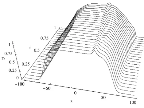
For comparison we also present the case of ζ =0 where the third-order dispersion term is absent, and in this case the initial anti-dark soliton decays very fast as a dispersive wave packet. The both case are presented in the following figures.

-100 -50 0 50 100 x 0.2 0.4 0.6 0.8 1 t 0 0.25 0.5 0.75 1 D 50 100

In the above figure we have the propagation of the anti-dark soliton atµ =0.3 . The anti-dark soliton stably propagates on the background wave and this figure has confirmed the existence of our result that the generalized nonlinear Schrödinger equation possesses the soliton solution in the small amplitude regime which is perfectly consistent with our theoretical analysis. It’s perfect to fit with our theoretical analysis. -100 -50 0 50 100 x 0.2 0.4 0.6 0.8 1 t 0 0.25 0.5 0.75 1 D 50 100

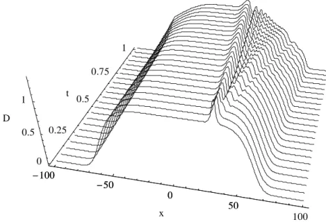
Fig. 2. The time evolution with the arbitrary coefficients whereµ =0.3, but the third-order dispersion term is absent.

In the Fig. 2 the third-order dispersion is absent that this figure is used to compare with Fig 1. It’s obviously that the solution of soliton we obtain only exists when we take into account the third order-dispersion term. Otherwise, the initial soliton wave packet will be dispersive rapidly as if a dispersive wave-packet. Therefore , we have confirmed our result by directly numerical simulation .

In this case with the same conditions as we choose the value of µ enough small , one can see the propagation of the anti-dark soliton steady , but in the larger

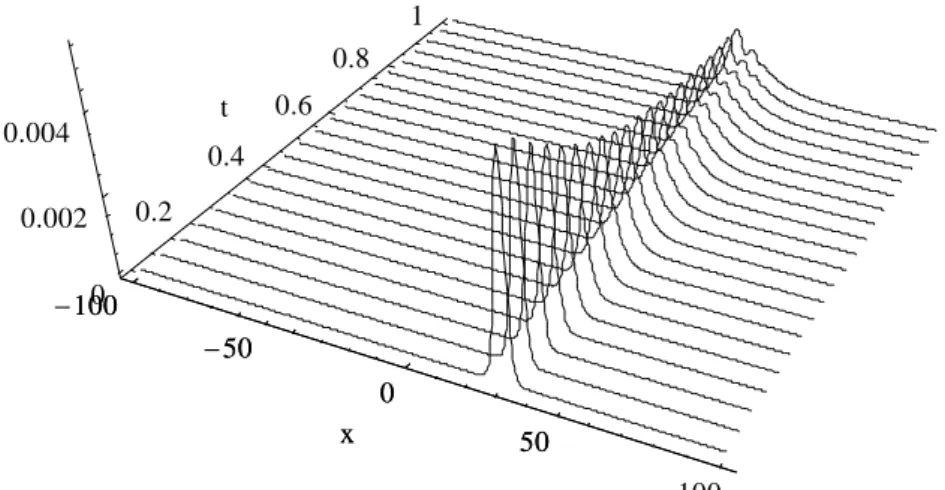
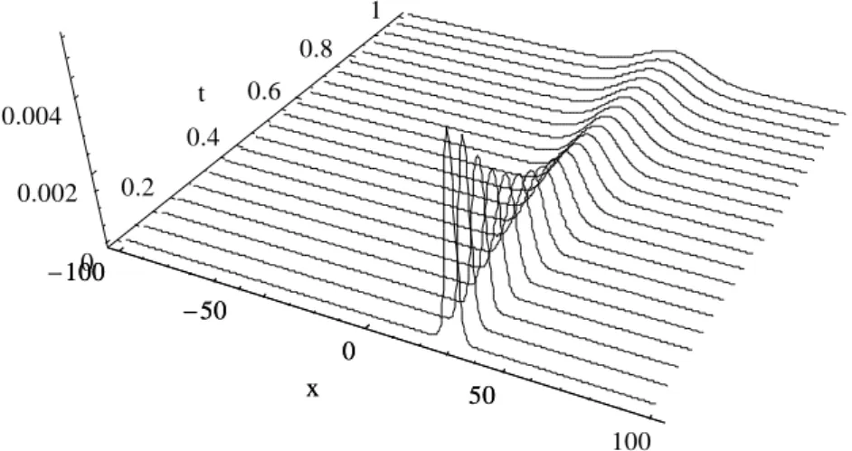
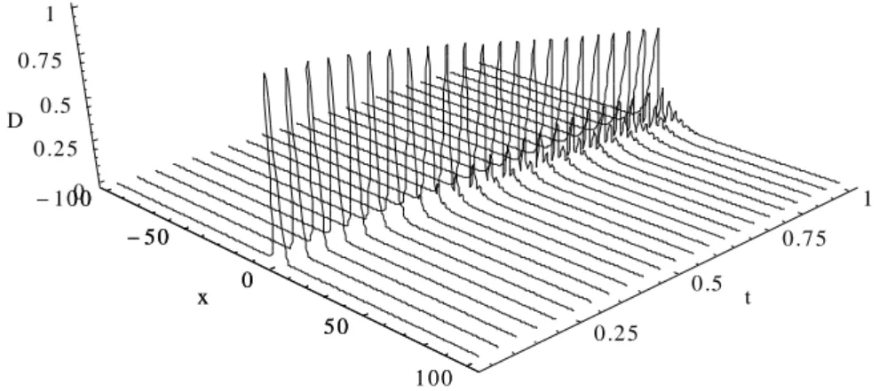
µ we will see an emission of radiation that is regarded as the effect of the third-order dispersion and had been studied in the optical fiber[16]. Now we discuss an instructive analysis to help us clearly understand the affection of the third-order dispersion term, even though it may don’t really exist any physical meaning. By erasing the background of the anti-dark soliton we just had discussed that we will take the form of bright soliton as an initial condition to substitute into our numerical simulation. The result is obviously to understand the affection of the third-order dispersion term in the following figure. In the figure 3 we clearly see the initial soliton form reshapes itself with an emission of continue radiation in a side. As for the figure 4 the wave is rapidly dispersive.

-100 -50 0 50 100 x 0.2 0.4 0.6 0.8 1 t 0 0.002 0.004 -100 -50 0 50 x

Fig. 3. The time evolution of a special initial profile which subtracts the background from the initial profile of fig. 1 with the same conditions

-100 -50 0 50 100 x 0.2 0.4 0.6 0.8 1 t 0 0.002 0.004 -100 -50 0 50 x

Fig. 4. The time evolution of a special initial profile which subtracts the background from the initial profile of fig. 2 with the same conditions.

As we change the ratio ofµ , the radiation will be more rapid and clearly observed. See the figure 5 whereµ =0.5.

-100 -50 0 50 100 x 0.2 0.4 0.6 0.8 1 t 0 0.01 0.02 0.03 0.04 100 -50 0 50 x