Vol. 39, No. 11, November 2001
Implicit Weighted Essentially Nonoscillatory Schemes
for the Compressible Navier
–
Stokes Equations
Jaw-Yen Yang¤
National Taiwan University, Taipei 10764, Taiwan, Republic of China
Yeu-Ching Perng†
Chung-Shan Institute of Science and Technology, Taoyuan 33509, Taiwan, Republic of China
and Ruey-Hor Yen‡
National Taiwan University, Taipei 10764, Taiwan, Republic of China
A class of lower–upper symmetric Gauss–Seidel implicit weighted essentially nonoscillatory (ENO) schemes for solving the two- and three-dimensional compressible Navier–Stokes equations with pointwise version of Baldwin– Barth one-equation turbulence model is presented (Baldwin, B. S., and Barth, T. J., “A One-Equation Turbulence Transport Model for High Reynolds Number Wall Bounded Flows,” AIAA Paper 91-0610,1991). A weighted ENO (WENO) spatial operator is employed for inviscid uxes and central differencing for viscous uxes. A numerical ux of the WENO scheme in ux limiter form is adopted, which consists of rst-order and high-order uxes and allows for a more exible choice of rst-order dissipative methods. The computations are performed for the two-dimensional turbulent ows over NACA 0012 and Royal Aircraft Establishment 2822 airfoil and the three-dimensional turbulent ow over an ONERA M6 wing. The present solutions are compared with experimental data and other computational results and exhibit good agreement.
I. Introduction
T
HE essentially nonoscillatory (ENO) schemes developed by Harten et al.1 are uniformly high-order accurate right up to discontinuities,while keeping a sharp, ENO shock transition.Later, Shu and Osher2;3devised an ef cient ux version. Since then, ENO schemes have been successfully applied to many different elds as noted in Ref. 4. However, they also have certain drawbacks. One problem is that the convergencerate for the implicit ENO scheme is generally poor. However implicit total variation diminishing(TVD) schemes5as constructed out of Harten’s TVD scheme6can achieve good convergence. Another problem is that an ENO scheme is not effective on vector supercomputers due to its heavy use of logical statements.Rogerson and Meiburg7 studied the convergence properties of ENO schemes, and they found that the numerical solution of ENO schemes does not converge uniformly. Shu8 proposed a modi ed ENO scheme, which recovers the correct order of accuracy for the test problem. A comparison of nite volume and nite difference implementation of high-order accurate ENO schemes was given by Casper et al.9
The weighted ENO (WENO) schemes proposed recently by Liu et al.10and extended by Jiang and Shu11can overcome these draw-backs while keepingthe robustnessand high-orderaccuracyof ENO schemes. The primary conceptof WENO schemes is that, insteadof using only one of the candidate stencils based on divided difference to form the reconstruction,one uses a convex combination of all of the candidate stencils. Each of the candidate stencils is assigned a weight that determines the appropriatecontributionof this stencil to the nal approximationof the numerical ux. Atkins12also devised a version of ENO schemes using a different weighted average of stencils. A class of implicit WENO schemes has been successfully applied to incompressible ow problems by Chen et al.13and Yang et al.14based on Chorin’s15arti cial compressibility formulation. Good convergencerate to a steady-statesolutionhas beenillustrated.
Received 4 October 1999; revision received 19 May 2000; accepted for publication 22 March 2001. Copyright c° 2001 by the American Institute of Aeronautics and Astronautics, Inc. All rights reserved.
¤Professor, Institute of Applied Mechanics, Department of Mechanical
Engineering; yangjy@spring. iam.ntu.edu.tw. Member AIAA.
†Research Scientist.
‡Professor, Department of Mechanical Engineering.
In this paper, following Chen et al.13and Yang et al.,14an implicit version of the WENO scheme (see Ref. 11) is adopted for the two-and three-dimensional compressible Navier–Stokes equations for computing steady-state ows. A numerical ux of WENO scheme in ux limiter form16is presented that consists of rst-order and high-order uxes and allows for a more exible choice of rst-order dissipative entropy satisfying methods. Many rst-order dissipative schemes can be used. Here, we employ the Roe scheme17 (with Harten’s entropy x6) as the basic rst-order dissipative methods.
For turbulent ow calculations, a pointwise version of the Baldwin–Barth one-equation turbulence model18 modi ed by Goldberg and Ramakrishnan19is adopted, which is based on the ·–" two-equation model. This model consists entirely of point-wise terms, that is, no term involves wall distance explicitly.Conse-quently, the resulting model provides a desirable tool for numerical computationof ow involvingcomplex geometry. The performance of this model has been tested through comparison with experimen-tal data of several well-documented ow cases, covering both wall-bounded and free shear ows.19
To improve the ef ciency and convergence to steady state, the lower–uppersymmetricGauss–Seidel (LU-SGS) implicitalgorithm (see Ref. 20) is adopted. It has been demonstrated by Yoon and Kwak21¡23 that the LU-SGS scheme requires less CPU time per iteration than most existing time marching methods on Cray super-computers. The LU-SGS scheme is not only unconditionallystable but also completely vectorizable in any dimensions. We apply the resulting schemes to compute standard transonic ows over NACA 0012 and Royal Aircraft Establishment (RAE) 2822 airfoils and three-dimensional transonic ow over ONERA M6 wing to test both the convergence rate and the accuracy of the methods.
II. Governing Equations
The governing equations are the unsteady, mass-averaged, com-pressible Navier–Stokes equations, which express the conservation of mass, momentum, and energy for a viscous gas. The pointwise version of the Baldwin–Barth one-equation turbulence model18as devisedin Ref. 19 is adopted.In the Cartesian coordinates,the three-dimensional governing equations are given by
@ Q @t C @ E @ x C @ F @ y C @ G @ z D @ Ev @ x C @ Fv @ y C @ Gv @z C H (1) 2082
where
Q D .½; ½u; ½v; ½w; e;R/T
E D [½u; ½u2C p; ½uv; ½uw; .e C p/u;Ru]T
F D [½v; ½vu; ½v2C p; ½vw; .e C p/v;Rv]T G D [½w; ½wu; ½wv; ½w2C p; .e C p/w;Rw]T (2) EvD M1 Re1 ³ 0; ¿x x; ¿x y; ¿xz; Ev5;¡¹ t ½¾" @R @ x ´T FvD M1 Re1 ³ 0; ¿xy; ¿yy; ¿yz; Fv5;¡¹ t ½¾" @R @ y ´T GvD M1 Re1 ³ 0; ¿xz; ¿yz; ¿zz; Gv5;¡¹t ½¾" @R @ z ´T (3) with Ev5D u¿x xC v¿x yC w¿x z¡ qx Fv5D u¿x yC v¿yyC w¿yz¡ qy Gv5D u¿xzC v¿yzC w¿zz¡ qz
In the preceding equations, ½ is the density; u, v, and w are the ve-locity components;e is the energy per unit volume; and the variable Rfor turbulence model is de ned by k2=", where k is the turbulent kinetic energy and " is the dissipation rate of k. The pressure p is related to the dependent variables by the equation of state for a perfect gas:
p D .° ¡ 1/[e ¡ ½.u2C v2C w2/=2] (4)
where ° is the ratio of speci c heats. The heat ux terms are given by qj D ¡.KlC Kt/@ T @ x j; j D 1; 2; 3 KlD ¹l .°¡ 1/Pr; Kt D ¹t .°¡ 1/Prt (5) where PrD 0:72 and PrtD 0:9 for air. The viscous stress tensors are
obtained from ¿i j D .¹lC ¹t/ ³ Si j ¡ 1 3 @uk @ xk±i j ´ (6) Si jD 1 2 ³ @ui @ xj C @uj @ xi ´ (7)
where i; jD 1; 2; 3 indicate the three coordinate directions. The molecular viscosity¹lis calculatedby Sutherland’s law. The source
term is expressed as
H D .0; 0; 0; 0; 0; H6/T
H6D .C"2f2¡ C"1/.RP/ 1
2C .M1=Re1/[¹lC .2¹t=¾"/]r2R¯½ where P is the production term of turbulent kinetic energy per unit mass and is given by
P D ReM1 1 ¹t "³ @ui @ xj C @uj @ xi ´ @ui @ xj ¡ 2 3 ³ @uk @ xk ´2#, ½
The quantities ¾", C"1, and C"2are empirical constants in the turbu-lence model: 1=¾"D .C"2¡ C"1/C 1 2 ¹ ¯ ·2 C"1D 1:2; C"2D 2:0; ·D 0:41; C¹D 0:09
and the eddy viscosity ¹tis given by
¹t D .Re1=M1/C¹½ f¹R De ne the turbulent Reynolds number ReTas
ReT ´ .Re1=M1/ ¡
½k2¯"¹l
¢
D .Re1=M1/½R=¹l
and the near-wall damping functions f2and f¹are expressed as
f2D 1 ¡ 0:3 exp ¡ ¡Re2 T ¢ ; f¹D 1¡ exp¡¡A¹Re2T ¢ 1¡ exp¡¡A"Re2T ¢ where A¹D 4:5 £ 10¡6; A"D C 3 4 ¹ ¯ 2·
Note that the near-wall functions f2 and f¹appearing in the pre-ceding formulation are not dependent on wall distance through the parameter yC.
The dimensional quantities (denoted by an overbar) are nondi-mensionalized using freestream conditions (denoted by1) and NL (the reference length used in the Reynolds number):
x D Nx=NL; y D Ny=NL; z D Nz=NL; t D NtNa1=NL
½D N½=N½1; u D Nu=Na1; vD Nv=Na1; wD Nw=Na1
a D Na=Na1; p D Np
¯
Np1Na21; T D NT=NT1 ¹lD N¹l=N¹l1; ¹t D N¹t=N¹l1; RD NR=NL Na1 whereNa1D .° Np1=N½1/1=2is the freestream speed of sound.
To allow for the development of a discrete control volume for-mulation, Eq. (1) is presented in integral form:
@ @t ³ 1 V Z V Q dV ´ C V1 I Ä .= ¡ =v/¢ n dÄ D H = D Ei C Fj C Gk; =vD Evi C Fvj C Gvk (8) where V is the volume of the cell that is bounded by the surface Ä with the outward unit normal n. Here we de ne the ux at general-ized coordinates (»; ´; ³ ) as
OE D .»xE C »yF C »zG/; OF D .´xE C ´yF C ´zG/
OG D .³xE C ³yF C ³zG/; OEvD .»xEvC »yFvC »zGv/ OFvD .´xEvC ´yFvC ´zGv/; OGvD .³xEvC ³yFvC ³zGv/ where »D »xi C »yj C »zk is the surface area vector in » direction.
III. Numerical Method and Boundary Conditions
Spatial Discretization
A semidiscrete nite volume method is used to ensure that the nal converged solution is independentof the integrationprocedure and to avoid metric singularity problems. The nite volume method is based on the local ux balanceof each mesh cell. The semidiscrete form of Eq. (8) can be written as
³ @ Q @t ´ i; j;k D ¡V1 h . QE ¡ QEv/i C1 2; j;k¡ . QE ¡ QEv/i ¡12; j;k i ¡V1 h . QF ¡ QFv/i; j C1 2;k¡ . QF ¡ QFv/i; j ¡12;k i ¡V1 h . QG ¡ QGv/i; j;k C1 2¡ . QG ¡ QGv/i; j;k ¡12 i C Hi; j;k (9)
where .i; j; k/ is the control point of nite volume. The spatial differencing adopts WENO schemes11for the inviscid convective uxes . QE; QF ; QG/ and second-order central differencing for viscous
in direction i can be put into the form of a ux limiter method16and is de ned by QEi C1 2; j;kD QE L i C1 2; j;kC QE H W i C1 2; j;k (10) where QEL is the numerical ux of a rst-order dissipative entropy
satisfying scheme (such as an E-scheme24and QEH Wis a high-order
ux with WENO2 ux limiter. Here the Roe scheme with Harten’s entropy x6is adopted: QEL i C12; j;kD 1 2 h OE¡Qi; j;k; Si C1 2; j;k ¢ C OE¡Qi C 1; j;k; Si C1 2; j;k ¢ ¡ .Rj3jR¡1/ i C12; j;k.Qi C 1; j;k¡ Qi; j;k/ i (11) where QE.Qi; j;k; Si C 1=2; j;k/ is the inviscid ux, the state variables at cell center .i; j; k/ and the area vectors at cell face .iC1
2; j; k/ are used. R is the similarity transformationmatrix consisting of the right eigenvectors of the Euler system linearized around the Roe-averaged state between Qi C 1; j;kand Qi; j;k.
QEH Wis a high-order WENO2 ux, de ned as
QEH W i C12; j;kD 6 X s D 1 QE¡H W i C12; j;k ¢ ;s¢ rs (12) QE¡H W i C12; j;k ¢ ;sD ¡ !C0;s¯2¢1E¡C i ¡1 2; j;k ¢ ;sC ¡ !C1;s¯2¢1E¡C i C1 2; j;k ¢ ;s ¡¡!¡0;s¯2¢1E¡¡ i C12; j;k ¢ ;s¡ ¡ !1;s¡¯2¢1E¡¡ i C32; j;k ¢ ;s (13) where 1E¡§ i C12; j;k ¢ ;sD ls¢ 1E § i C12; j;k (14) 1EC i C12; j;k D OE ¡ Q1 C 1; j;k; Si C1 2; j;k ¢ ¡ QEL i C12; j;k (15) 1E¡i C1 2; j;k D QE L i C12; j;k¡ OE ¡ Qi; j;k; Si C1 2; j;k ¢ (16) The weights !§are de ned by
!k;s§ D ®k;s§ ®0;s§ C ®1;s§ ; k D 0; 1 (17) where ®0;sC D 13 ¡ "C I SC 0;s ¢¡2 ; ®1;sC D 23 ¡ "C I SC 1;s ¢¡2 (18) ®0;s¡ D 23 ¡ "C I S¡ 0;s ¢¡2 ; ®1;s¡ D 13 ¡ "C I S¡ 1;s ¢¡2 (19) Here "D 10¡30and I S are the smoothness indicators, de ned as
I SC 0;sD ³ 1E¡C i ¡12; j;k ¢ ;s ´2 ; I SC 1;sD ³ 1EC¡ i C12; j;k ¢ ;s ´2 (20) I S¡ 0;sD ³ 1E¡¡ i C1 2; j;k ¢ ;s ´2 ; I S¡ 1;sD ³ 1E¡¡ i C3 2; j;k ¢ ;s ´2 (21)
In the preceding equations rs (column vector) and ls (row vector)
are the sth right and left eigenvectors of the Jacobian matrices, and they are evaluated using Roe17 averages. The r
s and ls used
in Eqs. (12) and (14), respectively, are evaluated consistently at the iC1
2 interface. Note that the WENO2 method just described is only second-order accurate because as a nite difference choice of uxes (dimensionby dimension) is appliedto a nite volume setting. However, it is still a genuinely second-order scheme, which does not degenerateto rst order at smooth extrema as TVD schemes do. The high-order ENO ux QEH E used for comparison in this work
is de ned as4 QE¡H E 1 C12; j;k ¢ ;s D 1 2m ³ 1E¡C i ¡1 2; j;k ¢ ;s; 1E C ¡ i C1 2; j;k ¢ ;s ´ ¡1 2m ³ 1E¡¡ i C12; j;k ¢ ;s; 1E ¡ ¡ i C32; j;k ¢ ;s ´ C ’PC ’M (22) where m.a; b/ D » a; if jaj · jbj b; if jaj > jbj (23) ’pD 1 6 8 > > > > > < > > > > > :
2m¡11EC.i¡ 1; j;k/;s; 11EC.i; j;k/;s¢ if 1EC¡i ¡1 2; j;k ¢ ;s · 1EC¡i C1 2; j;k ¢ ;s ¡m¡11EC.i; j;k/;s; 11EC.iC 1; j;k/;s¢ otherwise .24a/
’M D 1 6 8 > > > > > < > > > > > :
¡m¡11E¡.i; j;k/;s; 11E.i¡C 1; j;k/;s¢ if 1E¡¡i C1 2; j;k ¢ ;s · 1E¡¡i C3 2; j;k ¢ ;s 2m¡11E.i¡C 1; j;k/;s; 11E.i¡C 2; j;k/;s ¢ otherwise .24b/ The de nitions ofj1E§
.iC 1=2; j;k/;sj are the same as Eqs. (15) and (16) and 11E§
.i; j;k/;sare de ned as 11E.i; j;k/;s§ D 1E.i§C1
2; j;k/;s¡ 1E §
.i¡12; j;k/;s (25) Time Discretization
An unfactored implicit scheme can be obtained from a nonlinear implicit scheme by linearizing the ux vectors about the preceding time step and dropping terms of second and higher order:
[IC .1t=V /.±» OA C ±´ OB C ±³ OC/][I ¡ 1t OD]1Qi; j;k D ¡.1t=V / h . QE ¡ QEv/ni C1 2; j;k¡ . QE ¡ QEv/ n i ¡12; j;k i ¡ .1t=V / h . QF ¡ QFv/ni; j C1 2;k¡ . QF ¡ QFv/ n i; j ¡1 2;k i ¡ .1t=V / h . QG ¡ QGv/ni; j;k C1 2¡ . QG ¡ QGv/ n i; j;k ¡12 i C 1t Hi; j;k´ RHS (26)
where I is the identity matrix; n is the time level; ±»; ±´, and ±³are the differenceoperators, OA; OB, and OC are the Jacobianmatrices of
in-viscid uxes; OD D @ H=@ QI 1Q D Qn C 1¡ Qnand is the increment
of conservativevariables; and RHS is right-hand side. Note that the viscous terms are treated explicitly, and the turbulent source func-tions are treated implicitly. Because the production term is positive, its linearization is not possible; however, there is a strong coupling between the ow eld, turbulent viscosity, and the production term. The stiffness caused by the productionterm can be reducedby using the following pseudolinearization25:
@ H6 @R D ¡
jPj
0:1R (27)
The matrix inversion resulting from the source-term linearizationis performed before the spatial sweeps:
[IC .1t=V /.±» OA C ±´ OB C ±³ OC/]1Qi; j;k
D RHS=[I¡ 1t OD] ´ RHS¤ (28)
The LU-SGS implicit factorizationscheme of Yoon and Jameson20 for Eq. (28) can be derived by combining the advantages of LU factorizationand SGS relaxation.The LU-SGS scheme can be writ-ten as
where L D I C .1t=V /¡±»¡OACC ±¡ ´ OBCC ±³¡OCC¡ OA¡¡ OB¡¡ OC¡ ¢ D D I C .1t=V /. OAC¡ OA¡C OBC¡ OB¡C OCC¡ OC¡/ U D I C .1t=V /¡±C» OA¡C ±C ´ OB¡C ±C³ OC¡C OACC OBCC OCC ¢ where ±¡
»; ±¡´, and ±¡³ are backward differenceoperators and ±C»; ±C´, and ±C
³ are forward difference operators. Split Jacobian matrices of the ux vectorsare constructedso that the eigenvaluesofC matrices are nonnegative and those of¡ matrices are nonpositive, that is,
OA§D R
»3§»R¡1» ; OB§D R´3´§R¡1´ ; OC§D R³3§³R³¡1 where R»and R¡1» are similarity transformationmatrices of the eig-envectorsof OA. The Jacobianmatrices OA§
i C 1=2; j;kare computedusing the Roe-averaged17state between Q
i C 1; j;k and Qi; j;k and the area
vectors at cell face .iC 1
2; j; k/. Equation (29) can be inverted in three steps:
1Q¤D L¡1RHS¤ (30a)
1Q¤¤D DQ¤ (30b)
1Q D U¡1Q¤¤ (30c)
Note that the present implicit algorithm (LU-SGS) is completely vectorizable on iC j C k D const oblique plane of sweep. Boundary Conditions
The mean ow and turbulent transport equations presented in preceding sections represent an initia-boundary-valueproblem. To solve these equations,it is necessary to impose initial and boundary conditions.A uniform ow eld is chosenas the initialconditionsfor the mean ow equations. A uniform value ofR¼ 10¡4.ºt¼ 1000/ is set as the initial guess.
The boundary conditions of mean ow are set as follows: 1) No-slip boundary conditions for velocities are adopted on the solid surface, which is assumed to be an adiabatic wall. 2) The density and pressure on the wall are set to be equal to the values of the node points next to the wall. This gives rst-order accuracy at the wall. 3) In the far eld, a locally one-dimensional characteristic type of boundary condition is used. For the turbulent transport equation, a zeroth-order extrapolation is used to specify conditions at the far eld. The value ofRis set to zero at the solid wall.
IV. Results and Discussion
Presented here are the results of two different two-dimensional turbulent ows and one three-dimensional turbulent ow compu-tations to illustrate and test the codes. The two-dimensional cases are the transonic turbulent ows over NACA 0012 and RAE 2822 airfoil. The three-dimensionalcase is transonic turbulent ow over an ONERA M6 wing. We compare our results with available exper-imental data and other computational results for each case. Flow over NACA 0012 Airfoil
The rst result is the transonic ow over a NACA 0012 airfoil at freestreamcondition M1D 0:799; ® D 2:26 deg, and RecD 9£106.
The angle of attack (2.26 deg) used in the computation is obtained from the measured angle of attack (2.86 deg) using a linear wind-tunnel-wall correction procedure. For this transonic ow eld, a shock wave exists on the airfoil upper surface at about x=c D 0:5,
which is strong enough to cause signi cant boundary-layer sepa-ration. This case represents a severe test for all solution methods in terms of both numerical algorithm as well as turbulence models. The calculation is performed on an O-type grid. The grid system (Fig. 1) around the airfoil is 241 £ 45, with 113 points on upper surface, 113 points on lower surface and 17 points on blunt trailing edge, that is, base region, The mesh extends from the airfoil surface to a circle of the far- eld boundary located approximately 50 chord lengths from the body and the rst grid line at a distance of 7£10¡6 chord length off the wall, which resulted in a min yC< 1:5 over the entire grid; here yC< u
¿y=v, where u¿is the friction velocity.
Fig. 1 O-type grid 241 ££ 45 for NACA 0012 airfoil.
Fig. 2 NACA 0012 airfoil surface pressure distribution at M1 = 0:799;
® = 2:26 deg, and Rec= 9 ££ 106; comparison of WENO–Roe and ENO–
Roe schemes.
The solutions were calculated using WENO2–Roe and ENO2– Roe scheme, where Roe refers to the rst-order ux Roe scheme.17 The calculations presented here have been computed using local time steppingat constantCourantnumbersof 3.0. Figure 2 shows the comparison of surface pressure distributions with the experimental data.26The computed result is in good agreementwith experimental data exceptfor a slight discrepancyin the postshockpositionand the magnitude of lower surface pressure. Computed lift and drag coef- cients of WENO2–Roe scheme are CLD 0:335 and CDD 0:0325.
The experimentalvalues of lift and drag coef cients given by Harris are CLD 0:391 and CDD 0:033. Figure 3 shows the contours of
constant Mach numbers, all of the ow features including the front leading edge structure, the supersonic pocket, and shock separation are clearly resolved. Figure 4 shows the convergence history. Af-ter the residuals have decayed for three orders of magnitude, the convergence of ENO2 scheme is leveling off, whereas monotone convergence can be achieved with WENO2 schemes.
Flow over RAE 2822 Airfoil
The next computationis for the transonic ow over an RAE 2822 airfoil that has been tested extensively by Cook et al.27This airfoil is a supercritical airfoil with a signi cant amount of aft camber.
Fig. 3 Mach number contours for NACA 0012 airfoil at M1 = 0:799;
® = 2:26 deg, and Rec= 9 ££ 106; WENO2–Roe scheme.
Fig. 4 Convergence history for NACA 0012 airfoil at M1 = 0:799,
® = 2:26 deg, and Rec= 9 ££ 106.
Solutions were obtained of this case on four O-type meshes con-sisting of 241£ 45, 181 £ 45; 121 £ 45; and 177 £ 45 grid points in the streamwise and normal directions, respectively. The trailing edges of the rst three grid systems are blunt and that of the last grid system is sharp. The ne-grid system (Fig. 5) is similar to that used in the NACA 0012 airfoil test case.
The result is for the transonic ow over an RAE 2822 airfoil at freestreamcondition M1D 0:725, angle of attack® D 2:92 deg, and reference Reynolds number based on airfoil chord, RecD 6; 5 £ 106
corresponding to case 6 in the experimental study of Cook et al.27 Because of the presence of wall interference effects in the experi-ment, the corrected ow conditions with M1D 0:731 and ® D 2:51 as suggestedby Tatsumi et al.28are used. This ow involves a strong shock wave at x=c D 0:55 on the upper surface. The lift coef cient
in this case depends strongly on the predicted shock location. This requiresa goodresolutionof the shock wave. Jiang et al.29have com-puted this problem using convective upwind split pressure scheme with Baldwin–Barth one-equation turbulence model.18
In Fig. 6, the computed pressure coef cient distributions of the ne grid system of WENO2 and ENO2 schemes are shown and compared with the experiment. The present results are in close agreement with experimental data in all aspects. Figure 7 shows
Fig. 5 O-type grid 241 ££ 45 for RAE 2822 airfoil.
Fig. 6 RAE 2822 airfoil surface pressure distribution at M1 = 0:731;
® = 2:51 deg, and Rec= 6:5 ££ 106; comparison of WENO2 and ENO2
schemes.
Fig. 7 RAE 2822 airfoil surface pressure distribution at M1 = 0:731;
Table 1 Lift and drag coef cients for RAE 2822 airfoil at M1 = 0:725; ® = 2:92 deg, and Rec= 6:5 ££ 106
Scheme Grid Trailing edge CL CD
AGARD 0.743 0.0127 Jiang et al.29 384£64 0.702 0.0088 WENO2 241£45 Blunt 0.740 0.0151 WENO2 181£45 Blunt 0.737 0.0148 WENO2 121£45 Blunt 0.718 0.0138 WENO2 177£45 Sharp 0.738 0.0148 ENO2 241£45 Blunt 0.719 0.0149
Fig. 8 Skin-friction distribution of the upper surface of RAE 2822 airfoil at M1 = 0:731; ® = 2:51 deg, and Rec= 6:5 ££ 106; WENO2–Roe
scheme.
the results of the WENO2 scheme on different grid systems. A comparison of the calculated results of the experimental data and the Jiang et al.29results is shown in Table 1. Notice that the ow is grid resolved and that the sharp trailing edge produces almost the same solutionsas that obtained with a blunt trailingedge. Computed skin-friction distribution from the upper surface of the RAE 2822 airfoil for the case just presented is compared with experimental data in Fig. 8. The skin-frictionvalues are referred to the boundary-layer edge dynamic pressure. Generally, the computed results are in good agreement with experiment, with exceptions near the leading edge, where the skin-frictionquantity is dif cult to de ne, and near the trailing edge. The computed skin-friction coef cients by Jiang et al.29do not agree well with available experimental data. Figure 9 shows the contours of constant Mach numbers. Figure 10 shows the convergence history. Again, the WENO scheme gives a good convergencerate. Figure 11 shows the convergenceof lift and drag of the ne grid system of the WENO2–Roe scheme.
Our computed results for both the NACA 0012 and RAE 2822 airfoilsare consistentwith those given in the extensivecompendium of results by Holst.30
Three-Dimensional Transonic Flow over ONERA M6 Wing
The result of a three-dimensionalcase is the transonic ow over an ONERA M6 wing at a M1D 0:8395 and with 3.06-deg angle of attackand referenceReynoldsnumberRecD 2:6£106. The ONERA
M6 wing is a symmetric airfoil sectionwith a sweep angle of 30 deg. The wing is tapered with a taper ratio of 0.56 and has an aspect ratio of 3.8. Extensive wind-tunnel test data exist for the ONERA M6 wing, in particular,the pressure data for transonic ow conditions.31 Takakura et al.32have computed this problem using the Harten–Yee TVD scheme (see Ref. 5) together with the Jones–Launder k–" model.
Our calculation is performed on an O–O-type grid system, con-taining 160£ 25 £ 44 cells in the wraparound,spanwise, and body-normaldirections,respectively.The outer boundarieswere extended to a mesh system that extends to 30 chord lengths in all directions.
Fig. 9 Mach number contours for RAE 2822 airfoil at M1 = 0:731;
® = 2:51 deg, and Rec= 6:5 ££ 106; WENO2–Roe scheme.
Fig. 10 Convergence history for RAE 2822 airfoil at M1 = 0:731,
® = 2:51 deg, and Rec= 6:5 ££ 106.
Fig. 11 Convergence of lift and drag coef cients of WENO2–Roe scheme for RAE 2822 airfoil at M1 = 0:731; ® = 2:51 deg, and Rec=
Fig. 12 O-type grid 161 ££ 45 for ONERA M6 wing at symmetrical ( j = 1) plane. a) y/b = 0:44 b) y/b = 0:65 c) y/b = 0:80 d) y/b = 0:90
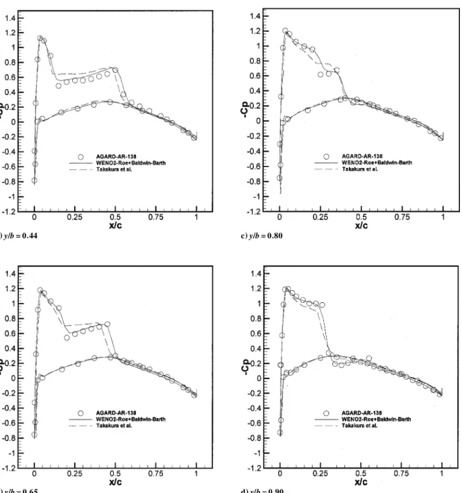
Fig. 13 Steady pressure distributions for ONERA M6 wing at M1 = 0:8395; ® = 3:06 deg, and Rec= 2:6 ££ 106.
The rst grid line is at a distance of 10¡5chord length off the wall, which resultedin a min yC< 2:0 over the entiregrid. The grid system was generated by letting the jD 1 plane (Fig. 12) be the plane of grid points on the upper wing surface at the root section. The j planes were then distributed nonlinearly along the upper surface to
j D 21 at the upper surface tip. Planes 22–26 were then rotated in a circular arc to model the wing tip. This wraparound wing tip al-lows the modeling of the wing tip as it existed in the wind-tunnel model.
The solutions were calculated using WENO2–Roe schemes at local Courant–Friedrichs–Lewy number 20.0. In Fig. 13, we show the surface pressure coef cients of the present scheme as compared with experimental data31 and the other calculations by Takakura et al.32(The number of grid points is 191£33£24:/ It is shown that our numerical results are in good agreement with the experimental data and are more accuratethan the results of Takakuraet al. in terms of both shock location and strength. This test case was at transonic condition, which results in a double-shockscon guration, which is evident in Figs. 13a–13c. Finally, Fig. 13d shows the shocks having coalesced to form one at the 0.25 chord position, and this shock is by far the strongest shock of all of those observed in Fig. 13. The con guration obviously results in the lambda double-shock
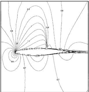
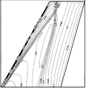
Fig. 14 Upper surface pressure contours for ONERA M6 wing at
M1 = 0:8395; ® = 3:06 deg, and Rec= 2:6 ££ 106.
Fig. 15 Convergence history for ONERA M6 wing at M1 = 0:8395;
® = 3:06 deg, and Rec= 2:6 ££ 106; WENO2–Roe scheme.
pattern for transonic conditions on a swept wing. Figure 14 shows the pressurecontoursalong the upper surface and the double-shocks pattern coalescing into a single shock at the tip can be observed. Figure 15 shows the convergence history.
V. Conclusions
High-resolution numerical codes for solving the two- and three-dimensional compressible Navier–Stokes equations with pointwise version of Baldwin–Barth18 one-equation turbulence model have been developed. The present method adopts a numerical ux in ux limiter form for the WENO spatial operator for convective ux that allows for a exiblility to implement various rst-order entropy satisfying dissipative schemes. The integration of equa-tions is via the implicit LU-SGS algorithm. Applicaequa-tions to tur-bulent transonic ows over NACA 0012 and RAE 2822 airfoils and three-dimensional turbulent ow over an ONERA M6 wing have been carried out to validate and illustrate the codes. The use of a WENO spatial operator for the inviscid uxes not only enhances the accuracy but also improves the convergencerate for steady-state
computation as compared with using the ENO counterpart. It is found that, for all cases computed, the solutions of the present algo-rithms are in good agreement with the experimental data and other available computational results.
Acknowledgments
This work was done under the auspices of National Science Council, Taiwan, throughGrant NSC-87-2212-E002-071.We thank Horng-Tsair Lee, Herng Lin, and Shih-Chang Yang of the Chung-Shan Institute of Science and Technology for many useful discus-sions. The authorswish to thank the reviewersfor many constructive comments and suggestions.
References
1Harten, A., Engquist, B., Osher, S., and Chakravarthy, S., “Uniformly
High-Order Accurate Nonoscillatory Scheme, III,” Journal of
Computa-tional Physics,Vol. 71, 1987, pp. 231–303.
2Shu, C.-W., and Osher, S., “Ef cient Implementation of Nonoscillatory
Shock Capturing Schemes,” Journal of Computational Physics, Vol. 77, 1988, pp. 439–471.
3Shu, C.-W., and Osher, S., “Ef cient Implementation of Nonoscillatory
Shock Capturing Schemes, II,” Journal of Computational Physics, Vol. 83, 1989, pp. 32–78.
4Shu,C.-W., “Essentially Oscillatory and WeightedEssentially
Non-Oscillatory Schemes for Hyperbolic Conservation Laws,” Advanced
Nu-merical Approximation of Nonlinear Hyperbolic Equations, edited by A. Quarteroni, Vol. 1697, Lecture Notes in Mathematics, Springer, 1998, pp. 325–432.
5Yee, H.-C., and Harten, A., “Implicit TVD Schemes for Hyperbolic
Con-servation Laws in Curvilinear Coordinates,” AIAA Journal, Vol. 25, No. 2, 1987, pp. 266–274.
6Harten, A., “A High Resolution Scheme for the Computation of Weak
Solutions of Hyperbolic Conservation Laws,” Journal of Computational
Physics,Vol. 49, 1983, pp. 357–393.
7Rogerson, A. M., and Meiburg, E., “A Numerical Study of the
Conver-gence Properties of ENO Schemes,” Journal of Scienti c Computing, Vol. 5, No. 2, 1990, pp. 151–167.
8Shu, C. W., “Numerical Experiments on the Accuracy of ENO and
Mod-i ed ENO Schemes,” Journal of ScientMod-i c Computing, Vol. 5, No. 2, 1990, pp. 127–149.
9Casper, J., Shu, C. W., and Atkins, H., “Comparison of Two
Formula-tions for High-Order Accurate Essentially Nonoscillatory Schemes,” AIAA
Journal,Vol. 32, No. 10, 1994, pp. 1970–1977.
10Liu, X.-D., Osher, S., and Chan, T., “Weighted Essentially
Nonoscil-latory Schemes,” Journal of Computational Physics, Vol. 115, 1994, pp. 200–212.
11Jiang, G.-S., and Shu, C.-W., “Ef cient Implementation of Weighted
ENO Schemes,” Journal of Computational Physics, Vol. 126, 1996, pp. 202–228.
12Atkins, H., “High-Order ENO Methods for the Unsteady Compressible
Navier–Stokes Equations,” AIAA Paper 91-1557, 1991.
13Chen, Y.-N., Yang, S.-C., and Yang, J.-Y., “Implicit Weighted ENO
Schemes for the Incompressible Navier–Stokes Equations,” International
Journal for Numerical Methods in Fluids, Vol. 31, 1999, pp. 747–765.
14Yang, J.-Y., Yang, S.-C., Chen, Y.-N., and Hsu, C.-A., “Weighted ENO
Schemes for the Three-Dimensional Incompressible Navier–Stokes Equa-tions,” Journal of Computational Physics, Vol. 146, 1998, pp. 464–487.
15Chorin,A. J., “A Numerical Methodfor SolvingIncompressibleViscous
Flow Problems,” Journal of ComputationalPhysics, Vol. 2, 1967, pp. 12–26.
16LeVeque, R. J., Numerical Method for Conservation Laws, Birkh¨auser
Verlag, 1990, p. 176.
17Roe, P., “Approximate Riemann Solvers, Parameter Vectors and
Dif-ference Schemes,” Journal of Computational Physics, Vol. 43, 1981, pp. 357–372.
18Baldwin, B. S., and Barth, T. J., “A One-Equation Turbulence
Trans-port Model for High Reynolds Number Wall-Bounded Flows,” AIAA Paper 91-0610, 1991.
19Goldberg, U.-C., and Ramakrishnan, S.-V., “A Pointwise Version of
Baldwin–Barth Turbulence Model,” ComputationalFluid Dynamics, Vol. 1, 1993, pp. 321–338.
20Yoon, S., and Jameson, A., “Lower-Upper Symmetric-Gauss–Siedel
Method for the Euler and Navier–Stokes Equaions,” AIAA Journal, Vol. 26, 1988, pp. 1025, 1026.
21Yoon, S., and Kwak, D., “Three-Dimensional Incompressible Navier–
Stokes Solver Using Lower–Upper Symmetric-Gauss–Seidel Algorithm,”
AIAA Journal,Vol. 29, 1991, pp. 874, 875.
22Yoon, S., and Kwak, D., “Implicit Navier–Stokes Solver for
Three-Dimensional Compressible Flow,” AIAA Journal, Vol. 30, 1992, pp. 2653– 2658.
23Yoon, S., and Kwak, D., “Multigrid Convergence of an Implicit
Sym-metric Relaxation Scheme,” AIAA Journal, Vol. 32, No. 5, 1994, pp. 950– 955.
24Osher, S., “Riemann Solver, the Entropy Condition, and Difference
Approximations,” SIAM Journal on Numerical Analysis, Vol. 21, 1984, pp. 984–995.
25Siikonen,T., “An Application of Roe’s Flux-Difference Splitingfor ·–"
Turbulence Model,” International Journal for Numerical Methods in Fluids, Vol. 21, 1995, pp. 1017–1039.
26Harris, C.-D., “Two-Dimensional Aerodynamic Characteristics of the
NACA0012 Airfoil in the Langley 8-Foot Transonic Pressure Tunnel,” NASA TM-81927, 1981.
27Cook, P.-H., McDonald, M.-A., and Firmin, M. C. P., “Airfoil RAE2822
Pressure Distributions and Boundary Layer and Wake Measurement,” AR-138-A6, AGARD, 1979.
28Tatsumi, S., Martinelli, L., and Jameson, A., “A New High
Resolu-tion Scheme for Compressible Flows Past Airfoil,” AIAA Paper 95-0466, 1995.
29Jiang, Y. T., Damodaran, M., and Lee, K. H., “High Resolution Finite
Volume Calculation of Turbulent Transonic Flow Past Airfoils,” AIAA Paper 96-2377, 1996.
30Holst, T. L., “Viscous Transonic Airfoil Workshop Compendium of
Results,” Journal of Aircraft, Vol. 25, 1988, pp. 1073–1087.
31Schimit, V., and Charpin, F., “Pressure Distributions on the ONERA
M6 Wing at Transonic Mach Numbers,” AR-138-B1, AGARD, 1979.
32Takarura, Y., Ogawa, S., and Ishiguro, T., “Turbulence Models for 3D
Transonic Viscous Flows,” AIAA Paper 89-1952, 1989.
P. Givi