Weighted Radial Basis Collocation Method for Boundary Value Problems

Weighted Radial Basis Collocation Method for Boundary Value Problems

H. Y. Hu1_{, J. S. Chen}2_{, and W. Hu}3

Submitted to

International Journal for Numerical Methods in Engineering

February 10, 2006

Abstract

This work introduces the weighted radial basis collocation method for boundary value problems. We first show that the employment of least-squares functional with quadrature rules constitutes an approximation of the direct collocation method. Standard radial basis collocation method, however, yields a larger solution error near boundaries. The residuals in the least-squares functional associated with domain and boundary can be better balanced if the boundary collocation equations are properly weighted. The error analysis shows unbalanced errors between domain, Neumann boundary, and Dirichlet boundary least-squares terms. A weighted least-squares functional and the corresponding weighted radial basis collocation method are then proposed for correction of unbalanced errors. It is shown that the proposed method with properly selected weights significantly enhances the numerical solution accuracy and convergence rates. Keywords: radial basis functions, collocation method, elasticity, least-squares method

1. Introduction

In the past two decades, there have been many applications for the radial basis functions, such as surface fitting, turbulence analysis, neural network, meteorology, partial differential equations and so forth. The originator of the radial basis function (RBF) is due to Hardy [8] for interpolation problems. Hardy [9] showed that multiquadrics RBF is related to a consistent solution of the biharmonic potential problem and thus has a physical foundation. Buhmann and Micchelli [1] and Chiu et al. [4] have shown that RBF are related to prewavelets (wavelets that do not have orthogonality properties). Madych and Nelson [17] proved that multiquadrics RBF and its partial derivatives have exponential convergence. The concept of solving partial

1_{Postdoctoral Fellow, Department of Mathematics, National Tsing Hua University, Hsinchu 30043, Taiwan. E-mail:} [email protected]

2 _{Corresponding Author, Professor, Department of Civil & Environmental Engineering, University of California,} Los Angeles, USA. E-mail: [email protected]

differential equations using RBF was first introduced by Kansa [12,13]. Franke and Schaback [7] provided some theoretical foundation of RBF method for solving PDE. Wendland [20] derived error estimates for the solution of smooth problems. Hu et al. [10] presented a radial basis collocation method including the combined and alternative schemes for singularity problems. Cecial et al. [2] gave a numerical scheme for Hamilton-Jacobi equations. Li [15] developed a mixed method for fourth-order elliptic and parabolic problems by using radial basis functions. Most RBFs with collocation lead to very ill-conditioned discrete systems. Wong et al. [19] suggested the use of multi-zone decomposition of domain. Kansa and Hon [14] observed that the condition numbers of the discrete system of direct collocation method can be greatly reduced by the domain decomposition. The shape parameter of RBF determines the locality of the RBF function and thus greatly influences the linear dependency and thus the condition number of the discrete system as reported by Schback and Hon [18]. Localized RBF have been introduced by Wendland [21] and truncated multiquadrics RBF have been proposed by Kansa and Hon [14] to reduce the bandwidth of the discrete system. Global and local RBFs have been investigated by Fasshauer [5] and smoothing methods and multilevel algorithm have been suggested.

Motivated by the aforementioned works, we are interested in the performance of radial basis collocation method in linear elasticity problems subjected to mixed Neumann and Dirichlet boundary conditions. In this work we first discuss how direct collocation method is related to the discrete least-squares method and the continuous least-squares method integrated by quadrature rule. The numerical results show that the standard collocation yields large numerical error on the boundaries. This is caused by the unbalanced least-squares residuals associated with domain and boundaries. To circumvent this deficiency, we propose to increase the weights of boundary collocation equations for enhanced numerical solution. The numerical investigation demonstrates that when proper weights on the boundary collocation equations are introduced, a much improved solution accuracy can be achieved.

This paper is organized as follows. In Section 2 we give a brief introduction of radial basis functions and their numerical properties. In Section 3, the direct collocation method of elasticity problem is introduced first. We then present the discrete least-squares method as an approximation of the overdetermined direct collocation equations. We also show that the discretization of continuous least-squares functional integrated with quadrature rule can yield the same discrete equation obtained from the discrete least-squares method with weighted inner product. To improve solution accuracy near the boundaries of the elasticity problems, the use of higher weights on the boundary collocation equations is also discussed in this section. Numerical examples are presented in Section 4, in which the effects of weights for domain and boundary collocation equations are studied, and the influence of RBF shape parameters on numerical solution is also investigated. Concluding remarks are given in Section 5.

2. Introduction to Radial Basis Functions (RBF)

Conventional finite element methods rely on the mesh topology to construct approximation functions. The numerical solution of these methods is extremely sensitive to the quality of mesh, and the construction of good quality mesh in complicated domain is a time consuming task.

Hardy [8] first investigated multiquadric RBF for interpolation problem, and Franke [6] showed good performance in scattered data interpolation using multiquatric and thin-plate spline radial basis functions. Since then, the advances of RBF to various problems have been progressed constantly. A few commonly used radial basis functions are listed below:

Multiquadrics (MQ):

( )

(

)

3 2 2 n ₂ I I g x = r +c − (2.1) Gaussian:

( )

(

)

2 2 3 2 2 2 ₂ 2 exp exp I I n _I I r c g r r c a −    −       =     _{+ −}    _{ }  x (2.2)

Thin plate splines:

( )

2 2 1 ln n I I I n I r r g r −  =   x (2.3) Logarithmic:

( )

n I I I g x =r ln r (2.4) where x=

(

x1 x2

)

,

(

(

) (

)

)

1 / 2 2 2 I 1 1I 2 2 I r = x −x + x −x in _{R , and} 2

(

)

I = x1I x2 I x is called the source point of RBF. The constant c involved in Eqns. (2.1) and (2.2) is called the shape parameter of RBF. In MQ RBF function in Eq. (2.1), the function is called reciprocal MQ RBF

if n=1, linear MQ RBF if n=2, and cubic MQ RBF if n=3, and so forth.

Madych [16] established several types of error bounds for multiquadric and related interpolators, Wu and Schaback [22] investigated local errors of scattered data interpolation by RBF in suitable variational formulation, and Yoon [23] regarded the convergence of RBF in an arbitrary Sobolev space. All of these studies show that there exists an exponential convergence rate in RBF. Moreover, one may consider RBF with variant shape parameter c in forms (2.1)-(2.2). Buhmann

and Micchelli [1] showed that the convergence rate is accelerated for monotonically ordered c.

Assume _{Ω ⊂R}2 _{is a closed region with boundary ∂Ω. Let S be a set of} s N source points, 1 2 [ , , _Ns] = ⊆ Ω ∪ ∂Ω S x x "x (2.5)

For a smooth function u x

( )

, the approximation, denoted by v

( )

x , is expressed by

( )

( )

1 s N I I I g a = =

∑

x x v (2.6)

where aI is the expansion coefficient. There exists an exponential convergence rate of RBF given by Madych [16]:

( ) ( )

( )

c / h

u x −v x ≈O η (2.7)

where 0< < is a real number, c is the shape parameter, and h is the radial distance defined as η 1

(

)

(

(

) (

)

)

:= I 1 / 2 2 2 1 1I 2 2 I h h sup min x x x x ∈ ∈Ω Ω, = − + − x S x S (2.8)

Note that η =exp

( )

−θ with θ >0 . The accuracy and rate of convergence of MQ-RBF approximation is determined by the number of basis functions (the number of source points) N _s

and the shape parameter c.

The application of RBF to partial differential equation is natural as the RBF are infinitely differentiable (g_I

( )

_{x ∈}C∞_):

( )

s

( )

n N n I I n n I 1 d d g a dx = dx =

∑

v x x (2.9)

3. Discretization of Boundary Value Problems by RBF Collocation Method

3.1 Strong Form

Consider the following general form of a boundary value problem

h h g g in on on = Ω = ∂Ω = ∂Ω Lu f B u h B u g (3.1)

where Ω is the problem domain, _{∂Ω is the Neumann boundary,} h _{∂Ω is the Dirichlet boundary,} g and _{∂Ω ∪ ∂Ω = ∂Ω , L is the differential operator in Ω ,} h g _{B is the differential operator on} h _{∂Ω ,} h and _{B is the operator on} g _{∂Ω .} g

For Poisson problem, L= ∆, h

n

∂ =

∂

B , 1_Bg _{= and u, f, h, and g are scalars. In linear elasticity,} the governing equations are given as

(

_{( , ) ,}

)

( , ) 0 ijkl k l _j i h ijkl k l j i g i i C u b in C u n h on u g on + = Ω = ∂Ω = ∂Ω (3.2)

where (C_ijkl =λδ δ_{ij kl} +µ δ δ_{ik jl}+δ δ_{il jk}) is the elasticity tensor, λ and µ are Lame’ constants, ( , )i j ( i j, j i,) / 2

u = u +u , u_{i j,} = ∂u_i/∂ , x_j b is the body force, _i n is the surface normal, _j h is the _i

surface traction, and g is the prescribed displacement. The operators _i L , _{B ,} h _{B and vectors u,} g

f, g, h corresponding to (3.2) in 2-dimensional elasticity are

(

)

(

)

(

)

(

)

2 2 2 2 2 1 2 1 2 2 2 2 2 2 1 2 2 1 2 2 x x x x x x x x λ µ µ λ µ λ µ λ µ µ  ₊ ∂ ₊ ∂ ₊ ∂   _{∂ ∂ ∂ ∂}    =  _{∂ ∂ ∂}  + + +   ∂ ∂ ∂ ∂     L ,

(

)

(

)

1 2 1 2 1 2 2 1 2 1 2 1 1 2 2 1 2 2 λ µ µ λ µ λ µ λ µ µ ∂ ∂ ∂ ∂  _{+ + +}   _{∂ ∂ ∂ ∂}    = ∂ ∂ ∂ ∂  _{+ + +}   _{∂ ∂ ∂ ∂}    h n n n n x x x x n n n n x x x x B , Bg =I _(3.3)

where I denotes the identity matrix and

1 2 1 2 1 2 1 2 [ , ] [ , ] [ , ] [ , ] T T T T u u b b h h g g = = − − = = u f h g (3.4)

3.2 Direct Collocation of Strong Form

For a multi-dimensional function u , the approximation by RBF defined at _i N source points, _s

denoted by vi is

( )

( )

( )

1 s N i i I iI I u g a = ≈ =

∑

x v x x (3.5) or 1 T 2   ≈ =_{ }=   u v a v Φ v (3.6) and

(

)

, ,

(

)

,

(

)

s s I T T T T T T 1 2 N I 1 2 N I 1I 2I I g 0 a a 0 g   = =_{ } = =   a a a a a " " Φ Φ Φ Φ Φ (3.7)

In collocation method, the residuals are enforced to be zeros at the collocation points. Let P be a

set of N collocation points in _p Ω , Q be a set of N collocation points on _{q ∂Ω , and R be a set} h of N collocation points on _{r ∂Ω ,} g 1 2 [ , , _Np] = ⊆ Ω P p p "p , [ , ,_{1 2 q}] h N = ⊆ ∂Ω Q q q "q , [ , ,1 2 r] g N = ⊆ ∂Ω R r r "r (3.8)

The source points set S and collocation points set P Q R may or may not have common ∪ ∪ points. By enforcing strong form of (3.1) to be satisfied at the collocation points, we have the following discrete equation:

= Aa b (3.9) where 1 2 3 =           A A A A ,

( )

(

)

( )

(

)

( )

(

)

( )

(

)

( )

(

)

( )

(

)

( )

(

)

( )

(

)

( )

(

)

T T T 1 1 1 T T T 2 2 2 1 2 3 T T T , , p q r h g h g h g N N N                         = = =                   _{ }     L p B q B r L p B q B r A A A L p B q B r # # # Φ Φ Φ Φ Φ Φ Φ Φ Φ (3.10) and 1 2 3     =       b b b b ,

( )

( )

( )

( )

( )

( )

( )

( )

( )

1 1 1 2 2 2 1 _, 2 _, 3 p q r N N N                   =_{ } =_{ } =_{ }             _{ }     f p h q g r f p h q g r b b b f p h q g r # # # (3.11)

For 2D linear elasticity, the entries of submatrices _{A ,} 1 _{A ,} 2 _{A are given by} 3

( ) (

₍

)

I ,11

( )

₎

J

_{( )}

I ,22

( )

J

₍

(

₎

_{( )}

)

I ,12

( )

J

_{( )}

1 IJ I J I ,12 J I ,22 J I ,11 J 2 g g g g 2 g g λ µ µ λ µ λ µ λ µ µ + + +   =  _{+ + +}    p p p A = L p p p p Φ (3.12)

( ) (

)

1 I ,1

_{( )}

( )

J 2

_{( )}

I ,2

( )

J

₍

1 I ,2

₎

( )

J

_{( )}

2 I ,1

( )

J

_{( )}

2 h IJ I J 2 I ,1 J 1 I ,2 J 2 I ,2 J 1 I ,1 J 2 n g n g n g n g n g n g 2 n g n g λ µ µ λ µ λ µ λ µ µ + + +   =  _{+ + +}    q q q q A = B p q q q q Φ (3.13)

( )

I

( )

J

_{( )}

3 g IJ I J I J g 0 g 0 g   =     r A = B r r (3.14)

The components of subvectors _{b b b are given by} 1_, 2_, 3 1 ( ) _, 2 ( ) _, 3 ( ) ( ) ( ) ( ) 1 J 1 J 1 J J J J 2 J 2 J 2 J -b h q -b h q       =_{ } =_{ } =_{ }       p q r b b b p q r (3.15)

In collocation method, typically the number of collocation points N_p +N_q+N_r is larger than the number of source points N , and hence the method yields an overdetermined system in Eq. (3.9). _s

This overdetermined system can be solved by QR decomposition, singular value decomposition, or least-squares method. For the least -squares approach, the overdetermined system is solved by minimizing the square of the Euclidean norm of the residual e Aa b= − :

(

) (

)

1 1 1 2 2 2 2 _T T Π = e = e e = Aa b− Aa b− (3.16) Minimizing Π requires

(

)

T ∂Π = − = ∂a A Aa b 0 (3.17) or T T A Aa = A b (3.18)

Here, solution of Eq. (3.18) is the least-squares approximation of the original solution of collocation method in Eq. (3.9). One can further consider a weighted inner product as

( )

_{, =} T

W

c d c Wd (3.19)

where W is a weight matrix:

) p q r 1 2 (N +N N w w w ₊       =         W % (3.20)

The weighted norm is defined as ⋅_W = ⋅ ⋅

( )

, _W1/ 2. Minimizing the weighted norm Π = e 2_W leads to the following equation:

T T

A WAa = A Wb (3.21)

Remark 3.1 Let a and a be the solution of Eq. (3.9) and Eq. (3.21), respectively. There exists a

(

T

)

T T cond ε − ≤ ⋅ ⋅ A W a a A WA a A Wb (3.22)

where ε = Aa - b , and Cond

( )

⋅ is the condition number of a given matrix in which the matrix norm is induced by the vector norm.

3.3 Least-Squares Functional

The discrete equation of original problem (3.1) can be obtained equivalently by discretization of the following functional

( )

1 ( ) ( ) 1 ( ) ( ) 1 ( ) ( ) 2 2 h 2 g T h T h g T g E d d d Ω ∂Ω ∂Ω =

_∫

L −f L −f Ω +

_∫

B −h B −h Γ +

_∫

B −g B −g Γ v v v v v v v (3.23)

The variational equation is obtained by the stationary condition of this functional to yield

( ) ( ) ( ) ( ) ( ) ( ) 0 h g T _d h T h _d g T g _d δ δ δ Ω ∂Ω ∂Ω − Ω + − Γ + − Γ =

∫

L v Lv f

∫

B v B v h

∫

B v B v g (3.24)

By introducing approximation of u using RBF in Eq. (3.6), and performing integration of Eq. (3.24) by quadrature rules in Ω and on _{∂Ω and} h _{∂Ω using collocation points, we have} g

( )

(

)

(

( )

)

( )

( )

(

)

(

( )

)

( )

( )

(

)

(

( )

)

( )

(

)

(

)

(

)

(

)

1 1 1 2 2 3 3 0 p q r T T T T T T N T T T T 1 I I I I I N T T h T h T 2 I I I I I N T T g T g T 3 I I I I I T 1 1 1 1 2 2 3 3 T T w w w δ δ δ δ δ = = =  −      + _ − _   + _ − _   = _ − + − + − _   = _ − _=

∑

∑

∑

a L p L p a f p a B q B q a h q a B r B r a g r a A W A a b A W A a b A W A a b a A W Aa b Φ Φ Φ Φ Φ Φ (3.25)

where A and b are given in Eqns. (3.10) and (3.11), 1 I

w , 2

I

w , and 3

I

w are the integration

weights in Ω , and on_{∂Ω and} h _{∂Ω , respectively, and} g 1 2 3     =       W W W W , 1 1 1 1 Np w w     =       W % , 2 1 2 2 Nq w w     =       % W , 3 1 3 3 Nr w w     =       % W (3.26)

For arbitrary admissible δa, the variational equation (3.25) yields Eq. (3.21). The above results

show that the least-squares residual method is an approximation of the direct strong form collocation method.

3.4 Modified Least-Squares Functional

Based on [11], we provide an error bound for the radial basis collocation method for elasticity. Denote V_Ns =span g g{ , , ,_{1 2} " g_Ns} a finite collection of RBF. This is a finite dimensional space belongs to a Sobolev space. Since v is a multi-dimensional function with dimension k,

( )

s s s s k N N N N V V V V V ∈ × × ×" = ≡ v (3.27)

We may define a norm as follows:

{

h g

}

1 2 2 2 2 h g 2 A = L 0 ,Ω+ 1,Ω+ B _{0 ,∂Ω} + B _{0 ,∂Ω} v v v v v (3.28)

wherev is the approximation of u, and k 2 2 i 1, 1, i 1 Ω Ω = =

∑

v v (3.29) L k ₂ 2 ij j 0 , 0 , i 1 Ω _Ω = =

∑

Lv v (3.30) h h k 2 2 h h ij j 0 , 0 , i 1 ∂Ω ∂Ω = =

∑

B v B v (3.31) g g k 2 2 g g ij j 0 , 0 , i 1 ∂Ω ∂Ω = =

∑

B v B v (3.32)

Let u be an optimal solution satisfying _Ns

( )

( ) inf s N _V E E ∈ = u v v (3.33)

We can obtain an estimate as follows: inf s h g N _{A V} A h g 1 _{0 ,} 2 _1, 3 _{0 ,} 4 _{0 ,} C C C _Ω C C ∈ Ω _{∂Ω ∂Ω} − ≤ − ≤ − + − + − + − u u u L f u B h B g v v v v v v (3.34)

Note that the existence and uniqueness of the solution follows immediately from Lax-Milgram lemma. The detailed analysis is omitted here. For the case of Poisson’s problem, we refer the reader to [11].

For Poisson problem for example, L= ∆, h

n

∂ =

∂

B , and _Bg _{=1, we have an error estimate}

(

)

(

)

(

)

(

)

(

)

: g s h g h g h N A 5 0 , 6 1, 7 8 0 , 0 , 5 0 , 6 1, 7 8 0 , 0 , 9 2, 7 n _{0 ,} 8 0 , 1 2 3 u u C u C u C h C g C u C u C u C u C u C u C u E E E Ω ∂Ω Ω ∂Ω Ω Ω ∂Ω ∂Ω Ω _∂Ω ∂Ω ∂ − ≤ ∆ − + − + − + − ∂ ∂ = ∆ − + − + − + − ∂ ≤ − + − + − = + + v v v v n v v v v n v v v (3.35)

Usually E E₁, ₂ >>E₃. Thus a modified norm is considered

(

h g

)

1 2 2 2 2 h h g g 2 B = L 0 ,Ω+ 1,Ω+α B 0 ,∂Ω +α B 0 ,∂Ω v v v v v (3.36) where h h k 2 2 h h h h ij j 0 , 0 , i 1 α α ∂Ω ∂Ω = =

∑

B v B v (3.37) g g k 2 2 g g g g ij j 0 , 0 , i 1 α _∂Ω α _∂Ω = =

∑

B v B v (3.38)

A corresponding error estimate is inf s h g N _{B V} B h h g g 1 0 , 2 1, 3 0 , 4 0 , C C C _Ω C α C α ∈ Ω ∂Ω ∂Ω − ≤ − ≤ − + − + − + − u u u L f u B h B g v v v v v v (3.39)

Similarly, for Poisson problem, we have the following error estimate:

(

)

(

)

(

)

g h s h g N B 5 2, 6 n 0 , 7 0 , h g 8 s _1, 9 _{n 2,} 10 _1, h g 8 s 11 s 10 1, u u C u C u C u C N u C u C u C N C N C u α α α α α α Ω ∂Ω ∂Ω Ω _Ω Ω Ω − ≤ − + − + − ≤ − + − + − ≤ + + − v v v v v v v (3.40)

in which the following inequalities have been used:

h n 0, 2, w _∂Ω ≤C w _Ω, s N w V ∀ ∈ (3.41) g 0 , 1, w _∂Ω ≤C w _Ω, ∀ ∈w V_Ns (3.42)

k s k , , w CN − w Ω ≤ Ω A A , k >A , ∀ ∈w VNs (3.43)

where C is a generic constant. To get a balance in error, the following relationship should be met:

( )

( )

h g

s

O 1 , O N

α ≈ α ≈ (3.44)

For the elasticity, the Lame’ constants λ and µ should be considered in the error estimates. Letting κ =max

{

λ µ,

}

, we obtain

(

)

h g s ' ' h ' g N _B C1κ _2,Ω C2κ α _{n 0 ,∂Ω} C3 α _{0 ,∂Ω} − ≤ − + − + − u u u v u v u v (3.45)

Further, this estimate can be further rewritten as

(

)

(

)

s ' ' N _B s 4 1 1 1, 5 2 2 1, ' h ' h s 6 1 1 1, 7 2 2 1, ' g ' g 8 1 1 1, 9 2 2 1, N C u C u N C u C u C u C u κ κ α α α α Ω Ω Ω Ω Ω Ω − ≤ − + − + − + − + − + − u u v v v v v v (3.46)

To get a balance in errors in elasticity, the following relationship should be met

( )

(

)

h g

s

O 1 , O N

α ≈ α ≈ κ (3.47)

Based on Eq. (3.39), we consider the following modified least-squares functional

( )

1 ( ) ( ) ( ) ( ) ( ) ( ) 2 2 h 2 g h g T h T h g T g E d α d α d Ω ∂Ω ∂Ω =

_∫

L −f L −f Ω +

_∫

B −h B −h Γ +

_∫

B −g B −g Γ v v v v v v v (3.48)

where _αh _{and α}g _{are weights for Neumann and Dirichlet boundary conditions, respectively.} Stationary condition of Eq. (3.48) gives rise to the following equation

(

)

(

)

T T T T T T 1 1 1 h 2 g 3 2 h 2 3 _{g 3} 1 1 1 h 2 g 3 2 h 2 3 _{g 3} α α α α α α α α    _{ }  _{ }  _{ }  _{ }  _{ }    _{ }  _{ } = _{ }    _{ }  _{ } A W A A A W A a W _A b W A A A W b W _b

The direct strong form collocation equation with weighted boundary conditions consistent to the weighted least-squares functional can be obtained by multiplying square root of weight numbers to the boundary equations in Eq. (3.1) to yield

1 1 h 2 h 2 g 3 g 3 α α α α           =              A b A a b A b (3.50)

4. Numerical Examples

In the following numerical analysis, we measure the solution accuracy by computing the L ₂

norm and _{H seminorm defined in (4.1) and (4.2), respectively, as follows:} 1

(

)(

)

1/ 2 0 i ui i u di Ω   − =_ − − Ω_ 

∫

 u v v v (4.1)

(

, ,

)(

, ,

)

1/ 2 1 i j ui j i j ui j d Ω   − =_ − − Ω_ 

∫

 u v v v (4.2) 4.1 Poisson equation

To examine the treatment of boundary conditions with the proposed method, we first solve the following Poisson equation:

( )

(

)

( ) ( )

( )

2 2 , 0,1 0,1 , xy xy u x y x y e u x y e ∆ = + Ω = × = ∂Ω (4.3)

The exact solution of this problem is _{e . The MQ-RBF is used as basis function:} xy

( )

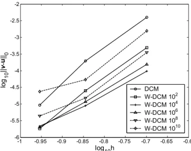
₂1 ₂ I I g r c = + x (4.4)

where shape parameter c=1.6 is used. Uniformly distributed 13 13× collocation points are used for 3 discretizations with 6x6, 8x8, and 10x10 source points. The results of direct collocation method (DCM) and weighted direct collocation method (W-DCM) with various weight _αg _for the boundary collocation equations are compared.

-1 -0.95 -0.9 -0.85 -0.8 -0.75 -0.7 -0.65 -0.6 -6 -5.5 -5 -4.5 -4 -3.5 -3 -2.5 -2 log₁₀h lo g10 ||v -u ||0 DCM W-DCM 102 W-DCM 104 W-DCM 106 W-DCM 108 W-DCM 1010

Figure 1. Convergence curves of direct collocation method and weighted direct collocation method with different weights

Figure 1 shows that W-DCM provides a better accuracy than that of the standard DCM. It is also shown that W-DCM with weight in the neighborhood _αg ₌₁₀4 _{yields best results. This} weighting value is consistent with the suggested value given in (3.44). As presented in Fig. 2 where c=1.6 and 8x8 source points with 13x13 collocation points are used, standard DCM leads to larger error near boundaries. The proposed W-DCM with _αg ₌₁₀4_{, on the other hand,} significantly improves solution accuracy of the problem.

We also compare the solutions obtained by the direct collocation method and least-squares method. Note that the condition number of the least-squares method is the square of the condition number of the direction collocation method. Thus a better solution accuracy in the direct collocation method is obtained than that of the least-squares method, especially for finer discretization. The situation is further magnified when higher weights are used for the boundary conditions in the weighted direct location method and the weighted least-squares method.

(a) DCM (b) W-DCM

g 4

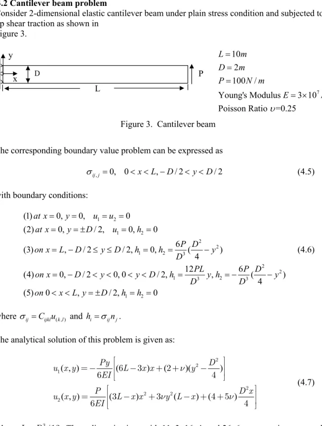
4.2 Cantilever beam problem

Consider 2-dimensional elastic cantilever beam under plain stress condition and subjected to a tip shear traction as shown in

Figure 3. 7 10 2 100 / Young's Modulus 3 10 Poisson Ratio =0.25 L m D m P N m E Pa υ = = = = ×

Figure 3. Cantilever beam The corresponding boundary value problem can be expressed as

, 0, 0 , / 2 / 2

ij j x L D y D

σ = < < − < < (4.5)

with boundary conditions:

1 2 1 2 2 2 1 2 3 2 2 1 3 2 3 1 2 (1) 0, 0, 0 (2) 0, / 2, 0, 0 6 (3) , / 2 / 2, 0, ( ) 4 12 6 (4) 0, / 2 0, 0 / 2, , ( ) 4 (5) 0 , / 2, 0 at x y u u at x y D u h P D on x L D y D h h y D PL P D on x D y y D h y h y D D on x L y D h h = = = = = = ± = = = − ≤ ≤ = = − = − < < < < = = − − < < = ± = = (4.6)

where σ_ij =C u_{ijkl ( , )k l} and h_i =σ_ijn_j.

The analytical solution of this problem is given as:

( , ) ( ) ( )( ) ( , ) ( ) ( ) ( ) Py D u x y L x x y EI P D x u x y L x x y L x EI ν ν ν     = − _ − + + − _       = _ − + − + + _   2 2 1 2 2 2 2 6 3 2 6 4 3 3 4 5 6 4 (4.7)

where I =D3/_{12 . Three discretizations with 11x3, 16x4, and 26x6 source points are used. The} collocation points of ( 2N₁− ×1) ( 2N₂− , where 1) N is the number of source points in the i-th _i

direction, are employed for the 3 discretizations. DCM and W-DCM with MQ-RBF are used in y

x

L

the numerical test, and the shape parameters c for the three discretizations 11x3, 16x4, and 26x6 are 30, 20, and 12, respectively.

With the guidance of error balance analysis in (3.47), weights for Dirichlet collocation equations g ₁₀9

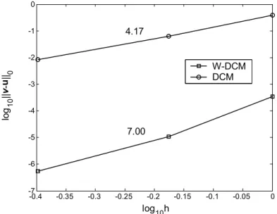
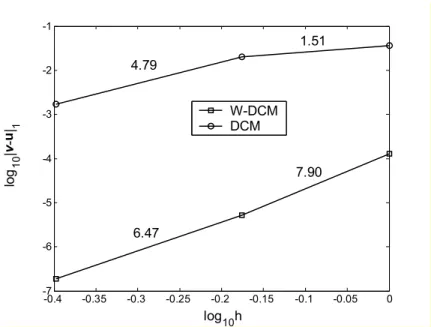
α = and Neumann collocation equations _αh _{=1 are used in W-DCM. Figures 4 and 5} compare the convergence of L norm ₂

0 h u u− and _{H seminorm} 1 1 h u u− , respectively. An enhanced solution accuracy is obtained using W-DCM.

Next, we compare the numerical solutions by using 3 sets of shape parameters c. Each set of c

parameters are selected to be linearly proportional to the nodal distance. The convergence properties presented in Fig. 6 suggest that there exists an optimal shape parameter for RBF collocation method.

Similar to the Poisson problem, the least-squares method produces a much larger condition number compared to that of the direct collocation method, and thus generates less accurate solution compared to the direct collocation method for both unweighted and weighted cases.

-0.4 -0.35 -0.3 -0.25 -0.2 -0.15 -0.1 -0.05 0 -7 -6 -5 -4 -3 -2 -1 0 log₁₀h log 10 ||v -u || 0 W-DCMDCM 7.00 4.17

-0.4 -0.35 -0.3 -0.25 -0.2 -0.15 -0.1 -0.05 0 -7 -6 -5 -4 -3 -2 -1 log₁₀h log 10 |v -u | 1 W-DCM DCM 4.79 1.51 6.47 7.90

Figure 5. Convergence of _H1 _seminorm

-0.4 -0.35 -0.3 -0.25 -0.2 -0.15 -0.1 -0.05 0 -6.5 -6 -5.5 -5 -4.5 -4 -3.5 -3 -2.5 log₁₀h lo g 10 ||v -u || 0 c = [ 25, 17, 10 ] c = [ 30, 20, 12 ] c = [ 100, 67, 40 ]

Figure. 6. Convergence in L₂ norm for different shape parameters c (three c values in each case

are associated with coarse, medium, and fine discretizations)

4.3 Infinite long cylinder subjected to an internal pressure

An infinite long (plane-strain) elastic cylinder is subjected to an internal pressure as shown in Fig. 7. Due to symmetry, only a quarter of the model (Fig. 8 (a)) is discretized by the RBF collocation method with proper symmetric boundary conditions specified. The corresponding boundary value problem can be expressed as

, 0, ij j in

with boundary conditions: 1 2 2 1 3 4 1 2 (1) , (2) , 0, 0 (3) , 0 (4) , 0, 0 i i i on h Pn on u h on h on u h Γ = − Γ = = Γ = Γ = = (4.9)

where σ_ij =C u_{ijkl ( , )k l} and h_i =σ_ijn_j. The analytical solution of this problem is given as

2 2 r 2 2 2 θ Pa r b u (r)= 1- ν + (1+ν) E(b - a ) r u (r)= 0         (4.10)

where_{E = E/ 1- ν ,}

(

2

)

_{ν = ν/ 1- ν}

₍

₎

_{, P is the internal pressure, b is the outer radius, and a is the inner} radius.

In this problem, both source points and collocation points are non uniformly distributed as shown in Fig. 8 (b). Three different discretizations, 7x7, 9x9, and 11x11 source points, are used, and the shape parameters c for three discretizations are 10, 7.5 and 6 respectively. The number of

corresponding collocation points is ( 2N₁− ×1) ( 2N₂ − , where 1) N is the number of source ₁

points along the radial direction and N is the number of source points along the angular ₂

direction.

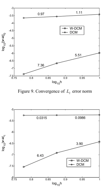
DCM and W-DCM with MQ-RBF are used in the numerical test. Weights for Dirichlet collocation equations _αg ₌₁₀9 _{and Neumann collocation equations α}h _{=1 selected based} on error analysis in (3.47) are used in W-DCM. The convergence of L norm ₂

0 h − u u and _H 1 seminorm 1 h −

u u obtained by DCM and W-DCM are compared in Figs. 9 and 10 respectively. As is shown in the numerical results, the direct collocation method with proper weights for Dirichlet and Neumann boundaries offer a much improved solution over the standard direct collocation method.

We also compare the numerical solutions by using 3 sets of shape parameters c. Due to the use of

non uniform discrete point distribution in this problem, each set of c parameters are selected to

be linearly proportional to the 1/

(

Ns − , where 1

)

N total number of source points. The s convergence properties presented in Fig. 11 again suggest that there exists an optimal shape parameter for RBF collocation method.

7 Inner radius: 4 Outer radius: 10 100 / Young's Modulus 3 10 Poisson Ratio =0.25 m m p N m E Pa υ = = ×

Figure 7. A infinite long cylinder subjected to an internal pressure

(a) (b)

Figure 8. (a) Quarter model, (b) Distribution of source points and collocation points in cylinder problem P Source point Collocation point Ω 1 Γ 2 Γ 3 Γ 4 Γ

0.75 0.8 0.85 0.9 0.95 1 -7.5 -7 -6.5 -6 -5.5 -5 -4.5 -4 -3.5 -3 log₁₀h lo g 10 ||v -u || 0 W-DCM DCM 7.36 5.51 0.97 1.11

Figure 9. Convergence of L error norm ₂

0.75 0.8 0.85 0.9 0.95 1 -8 -7.5 -7 -6.5 -6 -5.5 -5 log₁₀h lo g 10 |v -u | 1 W-DCM DCM 6.43 3.90 0.0315 0.0986 Figure 10. Convergence of 1 H seminorm

0.75 0.8 0.85 0.9 0.95 1 -7.4 -7.2 -7 -6.8 -6.6 -6.4 -6.2 -6 -5.8 -5.6 -5.4 log₁₀h log 10 ||v -u || 0 c = [ 6, 4.5, 3.6] c = [ 10, 7.5, 6 ] c = [ 20, 15, 12 ]

Figure. 11. Convergence in L2 norm for different shape parameters c (three c values in each case are associated with coarse, medium, and fine discretizations)

5. Concluding Remarks

This work introduces a weighted radial basis collocation method for boundary value problems. In this approach, the displacements are approximated by the radial basis functions, while the governing equation and boundary conditions are imposed directly at the collocation points. We first showed how direct collocation method is related to the discrete least-squares method constructed using least-squares residual of the discrete collocation equations. We then illustrated that by introducing a weighted inner product and the associated norm in the discrete least-squares method, the resulting discrete equation can be made identical to the discrete equation constructed by a continuous least-squares functional integrated with certain quadrature rule.

Standard collocation method introduces equal weights in the domain and boundary collocation points. The numerical results showed that with equal weights for the collocation equations associated with the domain differential equation and the boundary condition equations, the numerical error on the boundaries is significantly larger than that in the problem domain. Error analysis provided in this work indicates that the least-squares residual associated with differential equation in the domain is scaled by the number of source points compared with the least-squares residual associated with boundary conditions. By minimizing the total residual, larger error exists

on the boundary than that in the domain. In the case of elasticity, it can be shown that the domain and Neumann collocation equations are further scaled by the material constants. This existence of unbalanced errors in the collocation method can be enhanced by introducing the proper scaling weights for the Neumann and Dirichlet boundary collocation equations. The numerical results showed that by increasing the weights for the boundary collocation equations, the accuracy and convergence rates of the numerical solution are improved. In the case of elasticity, in particular, it is shown that due to the existence of Young’s modulus in the domain and

Neumann boundary collocation equations, the weight for the Dirichlet boundary collocation equations should be proportionally increased.

Since the condition number of least-squares method is the square of the condition number associated with the direct collocation method, the numerical solution obtained from the direct collocation method is generally better than that obtained by the least-squares method. This situation is even more transparent when comparing the weighted least-squares and weighted collocation methods.

The shape parameter in RBF plays an important role in the quality of numerical solution. Due to the use of collocation, employment of flatter (less localized) RBF functions is necessary for desired accuracy. This is analogous to the meshfree method where a very localized shape function with a direct nodal integration of weak form yields an unstable solution unless the kernel functions with large support size are used [3]. On the other hand, over flatted RBF functions increases dependency between the RBF functions and leads to an ill-conditioned discrete system. The numerical study showed that the adjustment of the shape parameters proportional to the nodal distance yields the better solution accuracy.

The main disadvantage of using RBF for solving partial differential equation is due to the non locality of the RBF function, which yields a full matrix in the discrete equation. On the other hand, localized RBF leads to an unstable solution similar to that observed in meshfree method with nodal integration [3]. This issue will be addressed in the forthcoming paper.

References

1. M. D. Buhmann and C. A. Micchelli, Multiquadric interpolation improved advanced in the theory and applications of radial basis functions, Comput. Math. Appl., Vol. 43, No. 12, pp. 21-25, 1992.

2. T. Cecil, J. Qian and S. Osher, Numerical methods for high dimensional Hamilton-Jacobi equations using radial basis functions, J. Comput. Physics, Vol. 196, pp. 327-347, 2004. 3. J. S. Chen, C. T. Wu, S. Yoon, Y. You, A Stabilized conforming nodal integration for

Galerkin meshfree methods,” International Journal for Numerical Methods in Engineering, Vol. 50, pp. 435-466, 2001.

4. C. K. Chiu, J. Stoeckler, and J. D. Ward, Analytic wavelets generated by radial functions, Adv. Comput. Math., Vol. 5, pp. 95-123, 1996.

5. G. E. Fasshauer, Solving differential equations with radial basis functions: multilevel methods and smoothing, Adv Comput. Math., Vol. 11, pp. 139-159, 1999.

6. R. Franke, Scattered sata interpolation: tests of some methods, Math. Comput., Vol. 98, pp. 181-200, 1982.

7. R. Franke and R. Schaback, Solving partial differential equations by collocation using radial functions, Applied Mathematics and Computation, Vol. 93, pp. 73-82, 1998.

8. R. L. Hardy, Multiquadric equations of topography and other irregular surfaces, J. Geophysics Res. Vol. 176, pp. 1905-1915, 1971.

9. R. L. Hardy, Theory and applications of the multiquadric-biharmonic method: 20 years of discovery, Comput. Math. Applic., Vol. 19, No. 8/9, pp. 163-208, 1990.

10. H. Y. Hu, Z. C. Li and A. H.-D. Cheng, Radial basis collocation method for elliptic equations, Computer Math. Applic., Vol. 50, pp. 289-320, 2005.

11. H. Y. Hu and Z. C. Li, Collocation methods for Poisson’s equation, Comput. Meth. Appl. Mech. Engng., in press, 2005.

12. E. J. Kansa, Multiqudrics - A scattered data approximation scheme with applications to computational fluid-dynamics - I Surface approximations and partial derivatives, Computer Math. Applic., Vol. 19, pp. 127-145, 1992.

13. E. J. Kansa, Multiqudrics - A scattered data approximation scheme with applications to computational fluid-dynamics - II Solutions to parabolic, hyperbolic and elliptic partial differential equations, Computer Math. Applic., Vol. 19, pp. 147-161, 1992.

14. E. J. Kansa and Y. C. Hon, Circumventing the ill-conditioning problem with multiquadric radial basis functions: Applications to elliptic partial differential equations, Vol. 39, No. 7/8, pp. 123-137.

15. J. Li, mixed methods for forth-order elliptic and parabolic problems using radial basis functions, Adv. Comput. Math., Vol. 23, pp. 21-30, 2005.

16. W. R. Madych, Miscellaneous error bounds for multiquadric and related interpolatory, Computer Math. Applic., Vol. 24, No.12, pp. 121-138, 1992.

17. W. R. Madych and S. A. Nelson, Multivariate interpolation and conditionally positive definite functions, II, Math. Comput., Vol. 54, pp. 211-230, 1990.

18. Y. C. Hon and R. Schaback and, On unsymmetric collocation by radial basis functions, Appl. Math. Comput., Vol. 119, pp. 177-186, 2001.

19. S. M. Wong, Y. C. Hon, T. S. Li, S. L. Chung, E. J. Kansa, Multi-zone decomposition of time-dependent problems using the multiquadric scheme, Comput. Math. Applic., Vol. 37, pp. 23-43, 1999.

20. H. Wendland, Meshless Galerkin methods using radial basis functions, Math. Comp., Vol. 68, No. 228, pp. 1521-1531, 1999.

21. H. Wendland, Piecewise polynomial, positive definite and compactly supported radial functions of minimal degree, Adv. Comput. Math., Vol. 4, pp. 389-396, 1995.

22. Z. Wu and R. Schaback, Local error estimates for radial basis function interpolation of scattered data, IMA J. Numer. Anal., Vol. 13, pp.13-27, 1993.

23. J. Yoon, spectral approximation order of radial basis function interpolation on the Sobolev space, SIAM J. Math. Anal., Vol. 33, No. 4, pp. 946-958, 2001.