The Spectrum of Chaotic Time Series (I): Fourier
Analysis
Goong Chen
1, Sze-Bi Hsu
2, Yu Huang
3, and Marco A. Roque-Sol.
1Abstract
The question of spectral analysis for deterministic chaos is not well understood in the literature. In this paper, using iterates of chaotic interval maps as time series, we analyze the mathematical properties of the Fourier series of these iterates. The key idea is the connection between the total variation and the topological entropy of the iterates of the interval map, from where special properties of the Fourier coefficients are obtained. Various examples are given to illustrate the applications of the main theorems.
Keywords: Li-Yorke chaos, topological entropy, total variation, Sobolev spaces, Fourier coefficients.
1 Department of Mathematics Texas A & M University, College Station, TX77843, U.S.A., Work completed while visiting Center for Theoretical Sciences, National Tsing Hua University, Hsinchu, Taiwan, R.O.C. E-mail: gchen@math.tamu.edu.
2 Department of Mathematics, National Tsing Hua University, Hsinchu, Taiwan, R.O.C. Supported in part by a grant from NSC of Rep. of China.
E-mail: sbhsu@math.nthu.edu.tw.
3 Department of Mathematics, Sun Yat-Sen (Zhongshan) University, Guangzhou 510275, P. R. China. Supported in part by Natural Science Foundation of Guangdong Province and the NSF of China. E-mail: stshyu@mail.sysu.edu.cn.
1
Introduction
Analysis of spectrum of a given functions is important in the understanding of function be-havior. Spectral analysis decomposes a function into a superposition of components, each with a special spatial and/or temporal frequency. Such a decomposition often reveals a cer-tain pattern of the frequency distribution. For example, the so-called “noise” is a function or process whose spectral decomposition has prominent, irregularly distributed high frequency
components. Spectral decomposition is a reversible process since by the inverse transform
or superposition we recover the original function. Thus, no information is lost from spec-tral decomposition. Superposition can be discrete or continuous. When the domain (e.g., an interval) is finite, spectrum of a function usually quantizes and is discrete. The Fourier trans-form or Fourier series expansion may be said to be the most basic method which constitutes the foundation of all the other spectral decomposition methods.
What kind of Fourier-spectral properties can we expect to have for a chaotic phenomenon ? This is the topic we want to address in this article. Here we are talking about deterministic chaos, which is an asymptotic time series represented by the iterates of a so-called chaotic interval map according to the definitions given in [3, 4, 15]. This topic is of obvious interest to many researchers. For instance, conducting a Google search by inputting “Fourier series of chaos”, we obtain well over 1,000 items. However, the greatest majority of such items study “Fourier series” and “chaos” disjointly. The rest of them are mostly of numerical simulation in nature. Very few analytical results concerning the Fourier spectrum of chaotic
time series exist so far, to the best of our knowledge.
Interval maps as mentioned in [4, 15] above are advantageous for doing mathematical analysis as chaos generated by them is comparatively simple and is quite well understood. There are various ways to characterize this type of chaos: positivity of Lyapunov exponents
or that of topological entropy, existence of homoclinic orbits or periodic points of specific order, etc. Here, our main tool is the total variation of a function. It is known [21] that the
topological entropy of a given interval map is positive (and, thus, the map is chaotic) if and only if the total variations of iterates of the map grow exponentially. This, together with cer-tain fundamental properties of Fourier series related to the total variation of a function, this enables us to obtain the desired interconnection between Fourier spectrum and chaos phe-nomena. Other properties ensue by the usual Lp properties and the topological conjugacy.
Basically, this paper may be viewed as a study of chaos for interval maps from an
integra-tion point of view, versus, say the Lyapunov exponent approach which is a differentiaintegra-tion
approach.
To be more precise and provide more heuristics, let I = [0, 1] be the unit interval and
f : I → I be continuous (called an interval map). Denote f°n = f ◦ f ◦ f ◦ · · · ◦ f : the n-th
iterative composition (or n-th iterate) of f with itself. Then the series f, f°2, f°3, . . . , f°n, . . .,
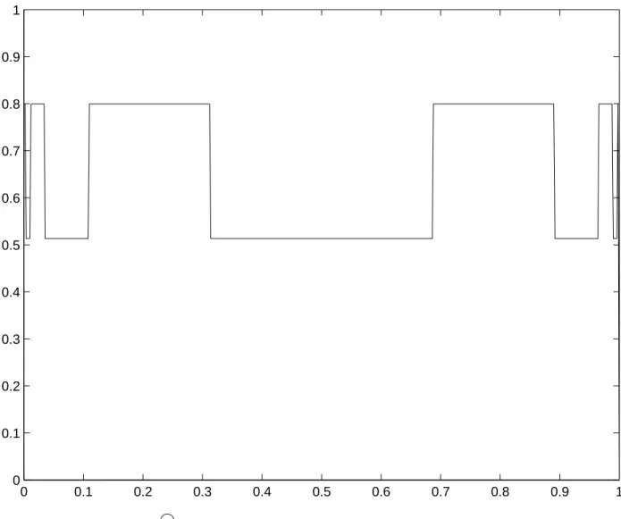
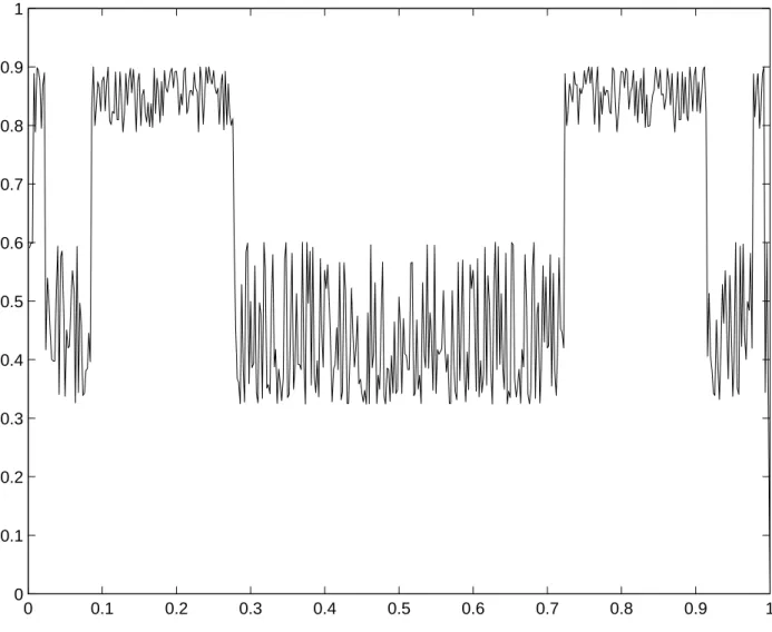
constitutes the time series we referred to in the above. Let us look at the profiles of two different cases, the first of which is nonchaotic and the second chaotic, as displayed in Figs. 1 and 2.
0 0.1 0.2 0.3 0.4 0.5 0.6 0.7 0.8 0.9 1 0 0.1 0.2 0.3 0.4 0.5 0.6 0.7 0.8 0.9 1
Figure 1: The profile f°100
µ on I, where fµ(x) = µx(1 − x) is the quadratic map (cf. Example
3.2), here with µ = 3.2, a case known to be nonchaotic. Note the nearly piecewise constant feature of the graph.
Our main question in this paper is: Can we analytically capture the highly oscillatory behavior of f°nfor a chaotic map f through the Fourier series of f°nwhen n grows very large?
The organization of this paper is as follows. In Section 2, we provide a recap of pre-requisite facts regarding interval maps and Fourier series. In Section 3, we offer three main theorems concerning Fourier series and chaos. Miscellaneous examples as applications are given in Section 4. A brief summary concludes the paper as Section 5.
This paper is Part I of a series. In Part II, we will discuss wavelet analysis of chaotic interval maps.
0 0.1 0.2 0.3 0.4 0.5 0.6 0.7 0.8 0.9 1 0 0.1 0.2 0.3 0.4 0.5 0.6 0.7 0.8 0.9 1
Figure 2: The profile of f°100
µ on I, where fµ is again the quadratic map, here with µ = 3.6,
a case known to be chaotic. Note that there are many oscillations in the graph, causing the total variations of f°n
µ to grow exponentially with respect to n and, thus, we call it the
2
Recapitulation of Facts about Interval Maps and
Fourier Series
This section recalls a brief summary of results needed for subsequent sections. For interval maps and chaos, we refer to the books by Devaney [15] and Robinson [23]. For Fourier series, cf. Edwards [16].
The concept of topological entropy, introduced first by Adler, Konheim and McAndrew [2] and studied by Bowen [5, 6, 7] is a useful indicator for the complexity of system behavior. Let X be a metric space with metric d. For S ⊂ X, define
dn,f(x, y) = sup
0≤j<n
d(f°j(x), f°j(y)); x, y ∈ S.
We say that S is (n, ε)−separated for f if dn,f(x, y) > ε for all x, y ∈ S, x 6= y. We use
r(n, ε, f ) to denote the largest cardinality of any (n, ε)−separated subset S of X.
Definition 2.1. Let (X, d) be a metric space and f : X −→ X be continuous. For any ε, the entropy of f for a given ε is defined by
h(ε, f ) = lim
n→∞
1
nln(r(n, ε, f )).
The topological entropy of f on X is defined by
h(f ) = lim
ε↓0h(ε, f ).
¤ Let X be a metric space and f : X → X be continuous. The nonwondering set of f (see, e.g., [25, p. 6]) Ω(f ) is an invariant subset of X. We have the following.
Theorem 2.1. [25, Proposition 8] Let f : X → X be a continuous map on a compact metric
space X. Let Ω ⊂ X be the nonwondering set of f . Then the topological entropy of f equals the entropy of f restricted to Ω, h(f ) = h(f |Ω). ¤
Theorem 2.2. Let f : I → I be an interval map. Then the following conditions are
equiv-alent:
(1) f has a periodic point of period not being a power of 2.
(2) f is strictly turbulent, i.e., there exist two compact subintervals J and K of I with
J ∩ K = φ and a positive integer k such that
f°k(J) ∩ f°k(K) ⊃ J ∪ K.
(3) f has positive topological entropy. (4) f has a homoclinic point.
(5) f is chaotic in the sense of Li–Yorke on the nonwandering set Ω(f ) of f . i.e., there
exists an uncountable set S contained in Ω(f ) such that
(i) lim sup
n→∞ d(f
°n(x), f°n(y)) > 0 ∀x, y, x 6= y, ∈ S.
(ii) lim inf
n→∞ d(f
°n(x), f°n(y)) = 0 ∀x, y, ∈ S.
¤ Let f : I → I be a chaotic interval map. Then for many examples, the graphs of the iterates f°n= f ◦ f ◦ · · · ◦ f (n times), n = 1, 2, 3, · · · , exhibit very oscillatory behavior. The
more so when n grows. A useful way to quantify the oscillatory behavior is through the use of total variations (cf. [8, p. 2164]). For any function f defined on I, we let VI(f ) denote the
total variation of f on I. If VI(f ) is finite, we say that f is a function of bounded variation.
We define the following function spaces:
BV (I, I): the set of all functions of bounded variation mapping from I to I;
Wk,p(I) = f ∈ D 0(I) | kf k k,p= " k X j=0 Z I |f(j)(x)|p dx #1/p < ∞ ,
for k = 0, 1, 2, . . . , 1 ≤ p ≤ ∞, where D0(I) is the space of distributions on I and
f(k) is the k-th order distributional derivative of f . The case p = ∞ is interpreted
in the sense of supremum a.e.
F1: the set of all functions f ∈ C0(I, I) such that f°n∈ BV (I, I) for n ∈ N
F2: the set of all functions f ∈ C0(I, I) such that f has finitely many extremal points.
It is clear that F2 ⊂ F1 and W1,∞(I, I) ⊂ F1.
Theorem 2.3. Let f ∈ F1. If f satisfies any conditions in (1)-(5) in Theorem 2.2, then
lim
n→∞
1
n ln(VI(f
°n)) > 0, (2.1)
i.e., VI(f°n) grows exponentially with respect to n. The converse is also true provided that
f ∈ F2. Indeed, for f ∈ F2, we have
h(f ) = lim n→∞ 1 nln(VI(f °n)). ¤ The proof of Theorem 2.3 can be founded in Misiurewicz and Szlenk [22]
Let f ∈ C0(I, I). The map f is called topologically mixing if, for every pair of nonempty
open sets U and V of I, there exists a positive integer N such that f°n(U) ∩ V 6= φ for all
n > N . And f is said to have sensitive dependence on initial condition on a subinterval J ⊂ I if there exists a δ > 0, called a sensitive constant, such that for every x ∈ J and
every open set U containing x, there exist a point y ∈ U and a positive integer n such that
Theorem 2.4. ([8, 19]) Assume that f ∈ F1. Then
(1) If f is topologically mixing, then VJ(f°n) grows exponentially as n → ∞ for any
subin-terval J ⊂ I;
(2) If f has sensitive dependence on initial data, then VJ(f°n) grows unbounded as n → ∞
for any subinterval J ⊂ I. The converse is also true provided that f ∈ F2.
(3) If f ∈ F2 and has sensitive dependence on initial data, then VI(f°n) grows exponentially
as n → ∞;
(4) If f has a periodic point of period four, then VI(f°n) grows unbounded as n → ∞. ¤
From Theorem 2.3 and 2.4, we know that the growth rates of the total variations of f°n
is strongly related to the dynamical complexity of f . The faster the total variations VI(f°n)
grow, the more fluctuations the graphs of f°nhave. This motivates us to define the following.
Definition 2.2. Let f ∈ F1. The map f is said to have chaotic oscillations (or rapid
fluctuation [13]) if VI(f°n) grows exponentially with respect to n, i.e., (2.1) holds. ¤
Obviously, if f ∈ F2 has chaotic oscillations, then f satisfies the definition of chaos given
in [4, 15].
Next, we recall some results about Fourier series. Let f ∈ L1(I). Denote
ck =
Z 1
0
e−2πikxf (x)dx, k ∈ Z. (2.2)
The Fourier series of f is defined to be
S(f )(ξ) =
∞
X
k=−∞
cke2πikξ, ξ ∈ R. (2.3)
The following is known to be true. Theorem 2.5. Let f ∈ L1(I) and let c
k be defined by (2.2). Then
(1) lim|k|→∞ck = 0, (the Riemann-Lebesgue Lemma).
(2) If f is differentiable at ξ0, then S(f )(ξ0) = f (ξ0) in the sense that
lim
M,N →∞ N
X
k=−M
cke2πikξ0 = f (ξ0), (Dirichlet’s Theorem).
(3) If f ∈ F1, then
2π|kck| ≤ |f (1) − f (0)| + VI(f ), k ∈ Z. (see Part II [9, Lemma 3.1]).
3
Main Theorems on the Fourier Spectrum of Chaotic
Time Series
Let f ∈ F1 and f°n be the nth iterates of f . Denote
cn k(f ) = Z 1 0 e−2πikxf°n(x)dx. (3.1) These numbers cn
k(f ) contain the complex magnitude and phase information of the Fourier
spectrum of the time series f°n, n = 1, 2, 3, · · · . Extensive numerical simulations by using
the fast Fourier transforms were performed by Roque-Sol [24]; see the good collection of graphics therein. Those graphics manifest a basic pattern that when f is a chaotic interval map, |cn
k(f )| have spikes when n and k are somehow related, as n and k both grow large.
Nevertheless, those numerical simulations do not offer concrete analytical results, as
aliasing effect significantly degrades numerical accuracy when the frequency (k in (3.1)) is
high, in any Fourier transforms. Also, Fourier components can only be computed up to, say
k = O(106), on a laptop, with uncertain accuracies.
Therefore, mathematical analysis is imperative in order to determine the spectral relation
cn
k between n and k.
Definition 3.1. Let φ : N ∪ {0} → N ∪ {0}. We say that φ grows exponentially if lim
n→∞
1
nln |φ(n)| ≥ α > 0, for some α.
¤ Main Theorem 1. Let f ∈ F1, and φ : N ∪ {0} → N ∪ {0} be an integer-valued function
growing exponentially, such that
lim n→∞ 1 n ln[|φ(n)c n ±φ(n)(f )|] > 0. Then lim n→∞ 1 n ln[VI(f °n)] ≥ α0 > 0, for some α0 > 0.
Consequently, f has chaotic oscillations.
Proof. Since f ∈ F1, f°n has bounded variation for any positive integer n. Applying
Theo-rem 2.5(3) to f°n, we have
2π|kcn
k(f )| ≤ |f°n(1) − f°n(0)| + VI(f°n), ∀k = ±1, ±2, . . . .
Now, let |k| = φ(n). Then, noting that |f°n(1) − f°n(0)| ≤ 2, we have
2 + VI(f°n) ≥ 2π|φ(n)cnφ(n)(f )|, implying lim n→∞ 1 n ln[VI(f °n)] ≥ lim n→∞ 1 nln[|φ(n)c n φ(n)(f )|] = α0 > 0, for some α0.
Remark 3.1. (1) If f ∈ F2 satisfies the assumptions in Main Theorem 1, then f has
positive entropy by Theorem 2.3.
(2) The assumptions in Main Theorem 1 are not necessary conditions for f to have chaotic oscillations. For instance, consider the map
f (x) = 3x if 0 ≤ x < 1 3, 1 if 1 3 ≤ x < 23, −3(x − 1) if 2 3 ≤ x ≤ 1 .
Then f ∈ F1. A simple computation shows that
V[0,1](f°n) = 2n.
So f has chaotic oscillations. But the corresponding Fourier coefficient cn
k(f ) satisfies |cnk(f )| ≤ Z I |f°n(x)|dx ≤ (2 3) n−1 → 0, as n → ∞. ¤
As an application of Main Theorem 1, we consider the tent map Tm(x) defined by
Tm(x) = ½ mx, 0 ≤ x < 1/m, m 1−m(x − 1), 1/m ≤ x ≤ 1. (3.2) Here, choose m = 2 so we have a full tent map T2(x), symmetric with respect to x = 1/2.
We have the following.
Theorem 3.1. For the (full) tent map T2(x) (with m = 2 in (3.2)), we have the Fourier
coefficients cn k(T2) given by cnk(T2) = ½ − 1 π2s2, if k = s2n−1, s = 1, 3, 5 . . . 0, otherwise.
Proof. See Appendix A.
Example 3.1. For the full tent map T2(x), if we choose
|k| = |s|2n−1 ≡ φ(n), s = 1, 3, 5 . . . ,
then by Theorem 3.1, we have lim n→∞ 1 nln[|φ(n)c n ±φ(n)(T2)|] = lim n→∞ 1 nln[s2 n−1 1 π2s2] = lim n→∞ 1 nln(2 n−1) = ln(2) > 0.
Remark 3.2. From the proof of our Main Theorem 1, we have lim n→∞ 1 nln[V1(f °n)] ≥ lim n→∞ 1 n ln[|φ(n)c n φ(n)(f )|]. (3.3)
On the other hand, for the full tent map T2(x), we have from Example 3.1
lim n→∞ 1 n ln[VI(T °n 2 )] = limn→∞ 1 nln[|φ(n)c n φ(n)(T2)|] = ln 2.
Thus inequality (3.3) is quite tight. ¤
The following two corollaries follow easily from Main Theorem 1.
Corollary 3.1. Under the assumption that f ∈ F1 and that φ : N ∪ {0} → N ∪ {0} grows
exponentially, and
|cn
±φ(n)(f )| ≥ β > 0 for n sufficiently large,
we have lim n→∞ 1 nln[VI(f °n)] ≥ α0 > 0 for some α0. ¤ Corollary 3.2. Let f ∈ F1. If VI(f°n) remains bounded with respect to n, then
lim
k→∞|c n
k(f )| = 0, (3.4)
uniformly for n. ¤
We know from Theorem 2.4 that f is not chaotic if VI(f°n) remains bounded with respect
to n.
Nevertheless, (3.4) is weaker than the condition lim
(n,k)→∞|c
n
k(f )| = 0. (3.5)
In fact, the boundedness of VI(f°n) with respect to n does not imply (3.5) in general. For
instance, f (x) = x, x ∈ [0, 1] = I, then f°n = f and V
I(f°n) = 1 for any n ∈ N, but
cn
k(f ) = c1k(f ) 6= 0, so (3.5) is violated.
Example 3.2. For the quadratic map fµ≡ µx(1 − x), x ∈ I, when 1 ≤ µ ≤ 3, satisfies that
VI(fµ°n) remains bounded for all n ∈ N. Thus, Corollary 3.2 applies. ¤
A somewhat generalized version of Main Theorem 1 may be given as follows. Theorem 3.2. Let f ∈ F1 and there exists a function φ : N → N such that
lim n→∞ 1 nln[φ(n)] ≡ α > 0. If lim n→∞ 1 nln " (φ(n))X k∈Z |cn k(f )|2sin2( kπ 2φ(n)) # > 0, (3.6)
then lim n→∞ 1 nln[VI(f °n)] = α0 > 0 for some α0. (3.7) In particular, if X k∈Z |cn k(f )|2sin2( kπ 2φ(n)) > 0,
then (3.6) holds and so does (3.7). ¤ The proof of this theorem can be obtained from the following lemma by setting r = φ(n) and g = f°n therein.
Lemma 3.1. [16, Exercise 8.13] Suppose g ∈ L2(I). Then
8rX k∈Z |c1 k(g)|2sin2( kπ 2r) ≤ Ω∞g( π r)VI(g),
for any positive number r, where
Ω∞g(a) = sup
0≤δ≤a
||Tδ(g) − g||C0, (Tδg)(x) ≡ g(x − δ),
and g is extended outside I by periodic extension. ¤ In most cases, it is quite impossible to calculate the Fourier coefficients explicitly for f°n
for a general interval map f . In the following, we derive a sufficient condition so that we do not need to compute the Fourier coefficients directly. Instead, we need some conditions on the derivative of the map.
Main Theorem 2. Let f ∈ W1,∞(I, I) satisfy
|f0| L∞(I) = γ > 0. If lim n→∞ 1 nln · X k∈Z |kcnk(f )|2 ¸ − ln γ > 0, (3.8)
then f has chaotic oscillations. Furthermore, if f ∈ F2, then f has positive topological
entropy and consequently, f is chaotic in the sense of Li-Yorke. Proof. We have 2πµ X k∈Z |kcn k(f )|2 ¶1/2 = · Z I |f°n0 (x)|1/2dx ¸2 ,
where “prime” denote the weak derivative of a given function. If |f0|
L∞(I) = γ, then we have
f°n0
(x) = f0(f(n−1)0
(x))f0(f(n−2)0
(x)) . . . f0(f (x))f0(x)
a.e. on I, and thus
|f°n0
We combine the above and now obtain 2πµ X k∈Z |kcn k(f )|2 ¶1/2 = · Z I |f°n0 (x)||f°n0 (x)|dx ¸1/2 ≤ · Z I γn|f°n0 (x)|dx ¸1/2 ≤ γn/2 · Z I |f°n0 (x)|dx ¸1/2 ≤ γn/2 · VI(f°n) ¸1/2 . Then 1 nln · X k∈Z |kcnk(f )|2 ¸ ≤ 1 n ln · ( 1 2π) 2γnV I(f°n) ¸ ≤ ln(γ) + 1 n ln · VI(f°n) ¸ − 2 nln(2π),
where the last term vanishes as n → ∞. By assumption, we obtain lim n→∞ 1 nln · VI(f°n) ¸ ≥ lim n→∞ 1 nln · X k∈Z |kcn k(f )|2 ¸ − ln(γ) > 0.
Therefore f has chaotic oscillations.
The second part of the theorem follows from Theorem 2.3.
Example 3.3. It follows from the proof of Main Theorem 2 that condition (3.8) is equivalent to lim n→∞ 1 nln · Z I |f°n0 (x)|2dx ¸ − ln(γ) > 0.
We consider the tent map Tm(x) as given in (3.2) with 1 < m ≤ 2. It is easy to see
that VI(Tm°n) = 2n for any m ∈ (1, 2]. Now we prove that the tent map Tm(x) satisfies the
assumptions in Main Theorem 2. We have Z I |Tm°n0(x)|2dx = µ m2 m − 1 ¶n . (3.9)
(See Appendix B for the proof.) For γ, we have γ = |T0| L∞(I) = max(m, m m − 1) = m m − 1, since 1 < m ≤ 2. Therefore lim n→∞ 1 nln · X k∈Z |kc1 k(Tm)|2 ¸ − ln(γ) = lim n→∞ 1 nln Z 1 0 |Tm°n0(x)|2dx − ln(γ) = [2 ln(m) − ln(m − 1)] − [ln(m) − ln(m − 1)] = ln(m) > 0, ∀1 < m ≤ 2. ¤
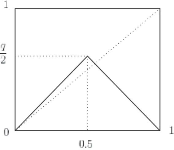
Example 3.4. Another example is to consider the triangular map Hq(x) defined by Hq(x) = ½ qx if 0 ≤ x < 1 2, q(1 − x) if 1 2 ≤ x ≤ 1,
where 0 < q ≤ 2. Fig. 3 show the graph of Hq(x) with 1 < q ≤ 2.
Figure 3: The graph of the triangular map Hq(x).
In this case, coefficients cn
k(Hq) are extremely hard to evaluate. But since γ = |Hq0|L∞ = q,
we have 1 n ln · X k∈Z |kcnk(f )|2 ¸ − ln(γ) = 1 nln · X k∈Z |kcnk(f )|2 ¸ − ln(q) = 1 nln · Z I |T°n0 (x)|2dx ¸ − ln(q) = 1 nln(q 2n) − ln(q) = 2 ln(q) − ln(q) = ln(q) > 0.
Thus the Triangular map Hq(x) has positive entropy when 1 < q ≤ 2 by applying Main
Theorem 2. ¤
What we have given so far in this section are sufficient conditions for chaos. But for a given function f ∈ W1,∞(I, I), there are some relations between V
I(f ) and ||f ||W1,∞(I,I),
which will allow us to state some necessary conditions. Proposition 3.1. Let f ∈ W1,∞(I, I). Then
VI(f°n) ≤ 2π[
X
k∈Z
|kcnk(f )|2]12.
Proof. Let f ∈ W1,∞(I, I) with the following Fourier series expansion
f (x) =X
k∈Z
c1
Then VI(f ) = Z 1 0 |f0(x)|dx ≤ µ Z 1 0 dx ¶1/2µ Z 1 0 |f0(x)|2dx ¶1/2 = µ Z 1 0 dx ¶1/2µ Z 1 0 |2iπX k∈Z kc1k(f )ei2πkx|2dx ¶1/2 ≤ 2πµ X k∈Z |kc1k(f )ei2πkx|2 ¶1/2 = 2πµ X k∈Z |kc1 k(f )|2 ¶1/2 .
Consequently, for the case of the nth iterates f°n of f , it follows that
VI(f°n) ≤ 2π µ X k∈Z |kcn k(f )|2 ¶1/2 .
Now, let us see how the Fourier coefficients of f°n and f°n0
behave when f has chaotic oscillations.
Main Theorem 3. (1) If f ∈ W1,∞(I, I) and f has chaotic oscillations, then
lim n→∞ 1 nln · X k∈Z |kcn k(f )|2 ¸ > 0.
(2) If f ∈ F2∩ W1,∞(I) and has positive entropy, then
lim n→∞ 1 nln · X k∈Z |kcn k(f )|2 ¸ > 0.
Proof. For (1), since f ∈ W1,∞(I, I) and W1,∞(I, I) ⊂ F
1, for any positive n, f°n has
bounded total variation. Assume that f has chaotic oscillations. Then 1
nln[VI(f
°n)] ≥ α > 0,
for some α. By Proposition 3.1, we have
2πµ X k∈Z |kcn k(f )|2 ¶1/2 ≥ VI(f°n). Thus lim n→∞ 1 nln · X k∈Z |kcnk(f )|2 ¸ = 2 lim n→∞ 1 nln · 2πµ X k∈Z |kcnk(f )|2 ¶1/2¸ ≥ lim n→∞ 1 n ln[VI(f °n)] = α > 0. (2) follows from (1) and Theorem 2.3.
We now consider the effects of topological conjugacy. Let f : I → I, g : J → J be continuous maps on compact intervals. We say f is topologically conjugate to g if there exists a homeomorphism h : I → J such that
hf = gh. (3.10)
Furthermore, if there exists a bi-Lipschitz h : I → J such that (3.10) holds, then we say f is Lipschitz conjugate to g. Without loss of generality, we assume J = I.
Recall that h : I → J is said to be bi-Lipschitz if both h and its inverse h−1are Lipschitz
maps. Thus f is topologically conjugate to g if they are Lipschitz conjugate to each other. Since topological entropy is an invariant of topological conjugacy, we have the following. Theorem 3.3. Let f : I → I and g : I → I belong to F2. If f is topologically conjugate to
g, then lim n→∞ 1 n ln · VI(f°n) ¸ = lim n→∞ 1 nln · VI(g°n) ¸ ,
in particular, f has chaotic oscillations iff g does. Proof. It follows from Theorem 2.3.
Theorem 3.4. Let f : I → I and g : I → I belong to F1. If f is Lipschitz conjugate to g,
then lim n→∞ 1 n ln · VI(f°n) ¸ = lim n→∞ 1 nln · VI(g°n) ¸ ,
in particular, f has chaotic oscillations iff g does.
Proof. The bi-Lipschitz property of h implies that h is strictly monotone. Assume that h is
strictly increasing. (If it is strictly decreasing, the proof is the same.) Thus, for any partition
x1 < x2 < · · · < xn on I, h(x1) < h(x2) < · · · < h(xn) is also a partition on I. So, we have n−1 X i=0 |f (xi+1) − f (xi)| = n−1 X i=0 |h−1(g(h(x i+1))) − h−1(g(h(xi)))| ≤ |h−1| Lip n−1 X i=0 |g(h(xi+1)) − g(h(xi))| ≤ |h−1|LipVI(g), where |h−1|
Lip is a Lipschitz constant. Therefore,
VI(f ) ≤ |h−1|LipVI(g).
By the same reasoning, we get
VI(f°n) ≤ |h−1|LipVI(g°n),
for any positive integer n. Thus lim n→∞ 1 n ln · VI(f°n) ¸ ≤ lim n→∞ 1 nln · VI(g°n) ¸ .
Since g°n is also Lipschitz conjugate to f°n for any positive integer n, by the same argument, we have lim n→∞ 1 n ln · VI(g°n) ¸ ≤ lim n→∞ 1 nln · VI(f°n) ¸ .
The proof is complete.
If the homeomorphism h in (3.10) is not bi-Lipschitz, we have the following
Main Theorem 4. Let f, g ∈ W1,∞(I) such that f and g are topologically conjugate: f =
h◦g◦h−1. Assume that h ∈ W1,p1(I) and h−1 ∈ W1,p2(I) for some p
1and p2: 1 < p1, p2 < ∞, satisfying either p1 > 1 p2− 1 or p2 > 1 p1− 1 . Let γ ≡ |f0|
L∞(I), such that
lim n→∞ 1 nln VI(g °n) − ln γ · p1 + p2 p1p2 > 0. Then lim n→∞ 1 nln VI(f °n) > 0
and f has chaotic oscillations. Proof. We have VI(g°n) = Z I |g°n0 |dx = Z I |h−1(f°n(h(x)))| · |f°n(h(x))| · |h0(x)|dx ≤ ·Z I |(h−1)0|p2 dx ¸1/p2·Z I |f°n0 (h(x))|q2|h0(x)|q2dx ¸1/q2 µ 1 q2 + 1 p2 = 1, i.e., q2 = p2 p2− 1 ¶ ≤ C1 ·Z I |f°n0 (y)|q2·p1−q2p1 dy ¸p1−q2 p1q2 ·Z I |h0(x)|p1 ¸1/p1 Ã C1 ≡ ·Z I |(h−1)0|p2dx ¸1/p2! = C2 ·Z I |f°n0(y)|p1−q2p1q2 dy ¸p1−q2 p1q2 Ã C2 ≡ C1· ·Z I |h0(x)|p2dx ¸ 1 p2 ! ≤ C2 ·Z I |f°n0(y)|dy · γn(p1−q2p1q2 −1) ¸p1−q2 p1q2 = C2[VI(f°n)] p1−q2 p1q2 · γn(1−p1−q2p1q2 ). (3.11) But p1 − q2 p1q2 = p1p2− (p1+ p2) p1p2 , 1 −p1− q2 p1q2 = p1+ p2 p1p2 ,
and inequality (3.11) gives lim n→∞ 1 nln VI(f °n) ≥ p1p2 p1p2− (p1+ p2) · lim n→∞ 1 nln VI(g °n) − ln γ · p1+ p2 p1p2 ¸ .
The proof follows.
Corollary 3.3. Assume the same conditions as Main Theorem 4, except that we have one
of the following three possibilities:
p1 = ∞, 1 < p2 < ∞; (3.12)
p2 = ∞, 1 < p1 < ∞, (3.13)
p1 = p2 = ∞. (3.14)
Then
(i) if (3.12) holds, we have lim n→∞ 1 nln VI(f °n) ≥ p2 p2− 1 · lim n→∞ 1 nln VI(g °n) − ln γ · 1 p2 ¸ ; (3.15)
(ii) if (3.13) holds, we have lim n→∞ 1 nln VI(f °n) ≥ p1 p1− 1 · lim n→∞ 1 nln VI(g °n) − ln γ · 1 p1 ¸ ; (iii) if (3.14) holds, then lim
n→∞
1
nln VI(f°n) > 0 iff limn→∞n1VI(g°n) > 0. ¤
Actually, case (iii) is Main Theorem 4.
Example 3.5. The quadratic map f4(x) = 4x(1 − x), where we choose µ = 4 in fµ (cf.
Example 3.2) is known to be topologically conjugate to the full tent map T2 (cf. Theorem
3.1): f4 = h ◦ T2◦ h−1, where h(x) = sin2³πx 2 ´ , h−1(y) = 2 πsin −1√y; x, y ∈ [0, 1]. We have h0(x) = π sinπx 2 cos πx 2 = π 2sin(πx) ∈ L ∞(I), (h−1)0(y) = 2 π 1 √ y 1 √ 1 − y ∈ L
i.e., p1 = ∞, p2 = 2 − δ, with 0 < δ < 1 for the purpose of the application of Corollary 3.2.
Here, γ = 2 for T2. Therefore, (3.15) gives
lim n→∞ 1 n ln VI(f °n 4 ) ≥ 2 − δ (2 − δ) − 1 · lim n→∞ 1 nln VI(T °n 2 ) − ln 2 · 1 2 − δ ¸ = 2 − δ (2 − δ) − 1 · lim n→∞ 1 n · (ln 2 n) − ln 2 · 1 2 − δ ¸ = 2 − δ 2 − (1 + δ) · ln 2 · µ 1 − 1 2 − δ ¶ > 0.
That is, f4 has chaotic oscillations.
Actually, it is straightforward to see that
VI(f4°n) = 2n and, thus, lim n→∞ 1 nln VI(f °n 4 ) = ln 2 > 0.
Here we show this example in order to motivate the applicability of Main Theorem 4 and Corollary 3.2 to possibly more general cases such as, e.g., small perturbations of h. ¤
4
Miscellaneous Consequences
We offer some examples as additional applications of the theory in Section 3.
Example 4.1 (Application to PDEs). Here, we show an application to the case of chaotic oscillations of the wave equation with a van der Pol nonlinear boundary conditions, as studied by Chen et al. [11] and Huang et al. [18, 19]. Consider the wave equation
wtt(x, t) − wxx(x, t) = 0, 0 < x < 1, t > 0, (4.1)
with a nonlinear self-excitation (i.e., van der Pol) boundary condition at the right end x = 1:
wx(1, t) = αwt(1, t) − βwt3(1, t), 0 ≤ α ≤ 1, β > 0,
and a linear boundary condition at the left end x = 0:
wt(0, t) = −ηwx(0, t), η > 0, η 6= 1, t > 0.
The remaining two conditions we require are the initial conditions
w(x, 0) = w0(x), wt(x, 0) = w1(x), x ∈ [0, 1].
Then using Riemann invariants
u = 1
2(wx+ wt),
v = 1
the above becomes a first order hyperbolic system ∂ ∂t µ u(x, t) v(x, t) ¶ = µ 1 0 0 −1 ¶ ∂ ∂x µ u(x, t) v(x, t) ¶ ,
where at the boundary x = 0 and x = 1 the reflection relations take place
v(0, t) = 1 + η
1 − ηu(0, t) ≡ G(u(0, t)),
u(1, t) = F (v(1, t)),
where F (x) ≡ x + g(x) and g(x) is the unique solution to the cubic equation
βg3(x) + (1 − α)g(x) + 2x = 0, x ∈ R.
Solutions wx(x, t), wt(x, t) of the wave equation display chaotic oscillatory behavior if G ◦ F
or equivalently F ◦ G is a chaotic interval map, when α, β, η lie in a certain region. We therefore deduce the following. Assume that for given α, β, η : 0 < α ≤ 1, β > 0 and η > 0, η 6= 1, the map G ◦ F is chaotic and that the initial conditions w0(·) and w1(·)
satisfy w0, w1 ∈ F2, and
w0 ∈ C2([0, 1]), w1 ∈ C2([0, 1]),
and that compatibility conditions
w1(0) = −ηw 0 0(0), w00(1) = αw1(1)βw31(1), w000(0) = −ηw01(0), w01(0) = [α − 3βw12(1)]w000(1), are satisfied. Then there exist A1 > 0, A2 > 0 such that if
|w00|C0(I), |w1|C0(I) ≤ A1 w
0
0 6= 0 or w1 6= 0,
then
|wx|C0(I), |wt|C0(I) ≤ A2.
In addition, we require that u(x, 0) and v(x, 0) take values in the “strange attractors” of
G ◦ F . Since G ◦ F and F ◦ G are chaotic, VI(u(·, t)) and VI(v(·, t)) grow exponentially with
respect to t. Therefore, VI(wx(·, t)) and VI(wt(·, t)) also grow exponentially with respect to
t. Since Z 1 0 |wxx(x, t)|dx = VI(wx(·, t)), Z 1 0 |wxt(x, t)|dx = VI(wt(·, t)), and · Z 1 0 |wxx(x, t)|2dx ¸1/2 ≥ Z 1 0 |wxx(x, t)|dx, · Z 1 0 |wxt(x, t)|2dx ¸1/2 ≥ Z 1 0 |wxt(x, t)|dx,
we obtain the following exponential growth results (stated in logarithmic form) lim n→∞ 1 nln · Z 1 0 µ |wxx(x, n + t0)| + |wxt(x, n + t0)| ¶ dx ¸ > 0, lim n→∞ 1 nln · Z 1 0 µ |wxx(x, n + t0)|2+ |wxt(x, n + t0)|2 ¶ dx ¸ > 0, for any t0 > 0.
Note that these estimates have not been obtainable by any other methods (such as the
energy multiplier method ). ¤
The chaotic behavior of the wave equation (4.1) with other boundary conditions have been also considered by Chen et al. [10, 12].
Example 4.2 (Entropy and Hausdorff dimension). Let X be a nonempty compact metric space and f : X → X a Lipschitz continuous map with Lipschitz constant L, that is,
∀x, y ∈ X, f satisfies
d(f (x), f (y)) ≤ d(x, y), where d is the metric of X.
The topological entropy h(f, Y ) of f on an arbitrary subset Y ⊂ X, given by Bowen [5], is much like the Hausdorff dimension, with the “size” of a set reflecting how f acts on it. Let
A be a finite open cover of X. For a set B ⊂ X we write B ≺ A if B is contained in some
element of A.
Let nf,A(B) be the largest nonnegative integer such that f°k(B) ≺ A for k = 0, 1, 2, . . . , nf,A−
1. If B ⊀ A then nf,A(B) = 0, and if fk(B) ≺ A for all k then nf,A(B) = ∞. Now, we
define
diamA(B) = exp(−nf,A(B)),
and DA(B, λ) = ∞ X i=1 (diamA(Bi))λ
for any family B = {Bi}∞1 of subsets of X and any λ ∈ R+. Define a measure µA,λ(Y ) by
µA,λ(Y ) = lim ε→0infB ½ DA(B, λ) : B = {Bi}∞1 , ∪Bi ⊇ Y, diamA(Bi) < ε ¾ ,
which has similar properties as the classical Hausdorff measure:
Hλ(Y ) = lim ε→0inf
½ X
i
(diam(Bi))λ: ∪iBi ⊇ Y and sup i
{|Bi|} < ε
¾
,
i.e., there exists h(f, Y, A) such that
µA,λ(Y ) = ∞ for λ < h(f, Y, A),
Finally, we define
h(f, Y ) = sup
½
h(f, Y, A) : A is a finite open cover of Y
¾
.
This number h(f, Y ) is the topological entropy of f on the set Y . If Y = X, then by [5, Prop. 1] we get
h(f, X) = h(f ),
the topological entropy of f . ¤
From Misiurewicz [21], we have the following.
Theorem 4.1. [21] For any Y ⊂ X, the Hausdorff dimension Hd(Y ) of Y , for a Lipschitz
continuous map f with Lipschitz constant L > 1, satisfies the inequality
Hd(Y ) ≥
h(f, Y )
ln(L) .
¤ Corollary 4.1. Under the same assumptions as in Theorem 4.1, the Hausdorff dimension
of X satisfies Hd(X) ≥ h(f, X) ln(L) = h(f ) ln(L), L > 1. ¤ Remark 4.1. More recently, Dai and Jiang [14] generalized Theorem 4.1 to the case that the phase space X is a metric space satisfying the second countability (but not necessarily compact).
Now, let us consider the case of an interval map f : I → I and let L the set defined by
L ={all Lipschitz continuous functions f : I → I, (4.2) with Lipschitz constant greater than 1}.
Theorem 4.2. Let W1,∞(I) ∩ F
2 ∩ L. Let cnk be the kth Fourier coefficient of f°n. If Ω(f )
denotes the set of nonwandering points of f , then
Hd(Ω(f )) ≥
1
ln(L)n→∞lim ln |kc n
k|, k = ±1, ±2, . . .
Proof. Apply Theorem 4.1 to Y = Ω(f ), which is an invariant, closed and therefore compact
set, and obtain
Hd(Ω(f )) ≥ h(f, Ω(f )) ln(L) = h(Ω(f )) ln(L) = h(f |Ω) ln(L) = h(f ) ln(L).
But we already know from (3) in Theorem 2.5 that 2 + VI(f°n) ≥ 2π|kcnk|. Therefore h(f ) = lim n→∞ 1 n ln[VI(f °n)] ≥ lim n→∞ 1 nln |kc n k|, implying Hd(Ω(f )) ≥ 1 ln(L)n→∞lim 1 nln |kc n k|.
Corollary 4.2. Let f be a function satisfying the hypotheses of Theorem 4.2, and let φ : N → N grow exponentially (satisfying Definition 3.1), and
lim
n→∞|c n
±φ(n)| > 0.
Then the Hausdorff dimension of the nonwandering set Ω(f ) is positive, i.e., Hd(Ω(f )) > 0.
Proof. Since φ : N → N grows exponentially, there are α1 > 0, α2 > 0 such that
φ(n) ≥ α1eα2n. By setting k = ±φ(n), we have lim n→∞ 1 nln |kc n k| = limn→∞ 1 nln |φ(n)c n ±φ(n)| = lim n→∞ 1 nln |α1e α2ncn ±φ(n)| = α2+ lim n→∞ ln(α1) n + limn→∞ ln |cn ±φ(n)| n = α2 > 0. Hence Hd(Ω(f )) ≥ 1 ln(L)n→∞lim 1 nln |kc n k| ≥ α2 ln(L) > 0.
In the case of the full tent map T2(x), the Lipschitz constant of T2(x) is obviously 2, i.e.,
L = 2.
Also, from Theorem 3.1 and Example 3.1, by choosing
φ(n) = s2n−1, s = 1, 3, 5, . . . , (4.3) we obtain
Hd(Ω(T )) ≥ ln(2)
Therefore
Hd(Ω(T )) = 1.
¤ Finally, we show an application of the Sturm-Hurwitz Theorem [20], an important the-orem in the oscillation theory of Fourier series, to the theory that we are developing here. Let X be a closed subset of the interval I = [0, 1] and f : X → X a continuous mapping. Denote J the set of all possible subintervals of I, and for J |Y the family of all subintervals
of I = [0, 1], each restricted to Y .
Definition 4.1. A cover A is called f -mono if A is finite, A ⊂ J |Y, and for any A ∈ A the
map f |A is monotone. ¤
Using the above definition we can see piecewise monotone functions in a slightly different way, namely, the following.
Definition 4.2. A map f is called piecewise monotone (p.m.), if there exists an f -mono
cover of X. ¤
Definition 4.3. Let f be a p.m. continuous mapping from an interval I into itself. Denote
ln = min
½
Card A : A is an f°n-mono cover ¾
, (Card means cardinality).
¤ From [22], we have the following.
Lemma 4.1. If f : I → I is a p.m. continuous map, then
htop(f ) = lim n→∞
1
nln(ln).
¤ The Sturm-Hurwitz Theorem says that if g : R → R is a continuous 2π-periodic function and dk is the kth Fourier coefficient of g, i.e.,
dk =
Z 2π
0
g(x)e−ikxdx, k = 0, ±1, ±2, . . . ,
and if k0 is the first nonzero Fourier coefficients of g, i.e.,
dk=
½
0 if |k| < k0,
6= 0 if |k| = k0,
Theorem 4.3. Let f ∈ C0(I, I) be a p.m. mapping with f (0) = f (1). If there exists a map
φ : N → N satisfying
ln[φ(n)] ≥ α1+ α2n, for some α1 ∈ R, α2 > 0,
such that the kth Fourier coefficient of f°n satisfies
cnk = ½ 0 if |k| < φ(n), 6= 0 for some |k| = φ(n), then htop(f ) > 0.
Proof. For a given n ∈ N define
gn(x) = f°n(
x
2π), x ∈ [0, 2π],
then gn(0) = gn(2π), so we can extend gn to the whole line R continuously with period 2π.
Applying the Sturm-Hurwitz Theorem, we have that gn(x) has at least 2φ(n) zeros in the
interval [0, 2π]. This implies that f°n has at least 2φ(n) distinct zeros in [0, 1]. Therefore
ln ≥ 2φ(n).
It follows from Lemma 4.1 that
htop(f ) = lim n→∞ 1 nln[ln] ≥ lim n→∞ 1 n · ln[2] + ln[φ(n)] ¸ ≥ lim n→∞ 1 n · ln[2] + α1+ α2n ¸ = α2 > 0.
Example 4.3. Consider T2(x), the full tent map. We can apply Theorem 4.3 by using
Theorem 3.1 and (4.3). The proof of Theorem 4.3 gives
htop(T2) ≥ ln 2.
Actually, htop(T2) = ln 2. ¤
5
Conclusions
Chaotic interval maps generate time series (constituted by their iterates) manifesting pro-gressively oscillatory behavior. Such oscillations must be reflected in the high order Fourier coefficients of the time series but no quantitative, analytical results were known previously. Our work here was first motivated by numerical simulation in [24]. Later, we recognized
some fundamental relation between coefficients of the Fourier series and the total variation of a given function (Theorem 2.5 (3)). Further, a concrete example (Theorem 3.1 and Exam-ple 3.1) was constructed. These have lead to a host of other related results and applications, yielding a form of “integration theory” for chaotic interval maps.
In Part II, we will continue the investigation by using wavelet transforms.
Appendix
A: Evaluation of the Fourier coefficients of T
2°n(x) for the tent map
T
2(x)
Here we present the Proof of Theorem 3.1.
The n − th iterate of the Triangular map T2(x) is given by
T2°n(x) = ½ 2nx − 2(l − 1), if 2(l−1) 2n ≤ x ≤ 2l−12n , −2nx + 2l, if 2l−1 2n ≤ x ≤ 22ln, for l = 1, 2, . . . , 2n−1. Now, cn k(T2) = 1 2 Z 1 0 T2°n(x)e−2πikxdx = 1 2 ½2n−1 X l=1 Z 2l−1 2n 2(l−1) 2n [2nx − 2(l − 1)]e−2πikxdx + 2n−1 X l=1 Z 2l 2n 2l−1 2n [−2nx + 2l]e−2πkxdx ¾ = 1 2 ½2n−1 X l=1 Z 2l−1 2n 2(l−1) 2n [2nx − 2(l − 1)]e−2πikxdx ¾ + 1 2 ½2n−1 X l=1 Z 2l 2n 2l−1 2n [−2nx + 2l]e−2πikxdx ¾ ≡ I1+ I2, where I1 = 1 2 ½2n−1 X l=1 Z 2l−1 2n 2(l−1) 2n [2nx − 2(l − 1)]e−2πikxdx ¾ = 1 2 ½2n−1 X l=1 Z 1 2 0 2te−2πikt+(l−1)2n−1 dt 2n−1 ¾ ; (2t = 2nx − 2(l − 1), dt = 2n−1dx) = 1 2 ½2n−1 X l=1 1 2n−2 Z 1 2 0 t[e−2n−2iπkt e− iπk(l−1) 2n−2 ]dt ¾
= 1 2 ½ 1 2n−2 Z 1 2 0 te−2n−2iπkt 2n−1 X l=1 e−iπk(l−1)2n−2 dt ¾ = 1 2 ½ 1 2n−2 Z 1 2 0 te−2n−2iπkt dt ¾2n−1 X l=1 e−iπk(l−1)2n−2 = 1 2n−1 ½ Z 1 2 0 te−2n−2iπktdt ¾2n−1 X l=1 e−iπk(l−1)2n−2 = ½ 2−2 −iπke − iπk 2n−1 + 2 n−3 π2k2(e − iπk 2n−1 − 1) ¾2n−1 X l=1 e−iπk(l−1)2n−2 and I2 = 1 2 ½2n−1 X l=1 Z 2l 2n 2l−1 2n [−2nx + 2l]e−2πikxdx ¾ = 1 2 ½2n−1 X l=1 Z 1 2 0 2te−2πik2n−1l−t dt 2n−1 ¾ ; (2t = −2nx + 2l, dt = −2n−1dx) = 1 2 ½2n−1 X l=1 1 2n−2 Z 1 2 0 t[e2n−2iπkt e− iπkl 2n−2]dt ¾ = 1 2 ½ 1 2n−2 Z 1 2 0 te2n−2iπkt 2n−1 X l=1 e−2n−1iπkl dt ¾ = 1 2 ½ 1 2n−2 Z 1 2 0 te2n−2iπkt dt ¾2n−1 X l=1 e−2n−2iπkl = 1 2n−1 ½ Z 1 2 0 te2n−2iπkt dt ¾2n−1 X l=1 e−2n−2iπkl = ½ 2−2 iπke iπk 2n−1 + 2 n−3 π2k2(e iπk 2n−1 − 1) ¾2n−1 X l=1 e−2n−2iπkl. Finally cn k(T2) = 1 2 Z 1 0 T2°n(x)e−2πikxdx = I1+ I2 = −2 n−3 π2k2(e iπk 2n−2)(1 − e− iπk 2n−1)2 2n−1 X l=1 e−2n−2iπkl.
Now, if k 6= s2n−1, s = 1, 2, . . . , then cn k(T2) = 1 2 Z 1 0 T2°n(x)e−2πikxdx = I 1+ I2 = −2 n−3 π2k2(e iπk 2n−2)(1 − e− iπk 2n−1)2 2n−1 X l=1 e−2n−2iπkl = −2n−3 π2k2(1 − e −i2πk) ½ 1 − e−2n−1iπk 1 + e−2n−1−iπk ¾ = 0.
On the other hand, if k = s2n−1, s = 1, 3, 5, . . . , then
cn k(T2) = 1 2 Z 1 0 T2°n(x)e−2πikxdx = I 1+ I2 = −2 n−3 π2k2(e iπk 2n−2)(1 − e− iπk 2n−1)2 2n−1 X l=1 e−2n−2iπkl = − 1 π2s2
B: Some calculations for T
°nm
(x) needed for Example 3.3
Here we present the Proof of (3.9)
Consider the tent map given by (3.2), i.e.,
Tm(x) = ½ mx, 0 ≤ x < 1/m, m 1−m(x − 1), 1/m ≤ x ≤ 1, for 1 < m ≤ 2.
Tm has an extremal point x = a12 = m1, as displayed in Fig. 4.
After iterating Tm twice, Tm°2 has three extremal points:
a2 2 = a11+ 1 m(a 1 2− a11) = 1 m2, a2 3 = a12, a2 4 = a13+ 1 m(a 1 2− a13) = 1 + 1 m( 1 m − 1). See Fig. 5.
After n iterates, if we denote by an
l, l = 2, 3, · · · , 2n, the extremal points of Tm°n and let
an
1 = 0, an2n+1 = 1, be the two boundary points, then we have
an 2l−1= an−1l , l = 1, 2, · · · , 2n−1+ 1, an 2l = ½ an−1 l +m1(an−1l+1 − an−1l ), if l is odd, an−1l+1 + 1 m(a n−1 l − an−1l+1), if l is even,
Figure 4: The graph of the tent map Tm.
Figure 5: The graph of the tent map T2
m. for l = 1, 2, · · · , 2n−1. Thus an2l− an2l−1= λλbl(1 − λ)(n−1)−bl, (5.1) an 2l+1− an2l = (1 − λ)λbl(1 − λ)(n−1)−bl, (5.2) where λ = 1 m, 1 < m ≤ 2, l − 1 = cn−22n−2+ cn−32n−3+ · · · + c121+ c0,
the binary expansion of l − 1, with cj = 0 or 1,
bl = number of zeroes in thebinary coefficients
On the other hand, we know that Tm°n0 = 1 an 2l− an2l−1 , on (an2l−1, an2l), Tm°n0 = − 1 an 2l+1− an2l , on (an2l, an2l+1).
It follows from (5.1) and (5.2) that Z 1 0 |T(n0) m |2dx = 2n−1 X l=1 · Z an 2l an 2l−1 1 (an 2l− an2l−1)2 dx + Z an 2l+1 an 2l 1 (an 2l+1− an2l)2 dx ¸ = 2n−1 X l=1 · 1 an 2l− an2l−1 + 1 an 2l+1− an2l ¸ = 2n−1 X l=1 1 λbl+1(1 − λ)n−bl = n−1 X b=0 µ n − 1 b ¶ 1 λb+1(1 − λ)n−b = · 1 λ(1 − λ) ¸n = µ m2 m − 1 ¶n . Thus (3.9) holds.
References
[1] R.A. Adams and J.F. Fournier, Sobolev Spaces, 2nd ed., Elsevier, Amsterdam, 2003.
[2] R.L. Ader, A.G. Konheim and M.H. McAndrew, Topological entropy, Trans. Amer. Math. Soc. 114, 309-319, (1965).
[3] J. Banks, J. Brooks, G. Cairns, G. Davis and P. Stacy, On Devaney’s definition of chaos, Amer. Math. Monthly 99, 332-334, (1992).
[4] L.S. Block and W.A. Coppel, Dynamics in One Dimension, Lecture Notes in Mathe-matics 1513, Springer-Verlag, New York, 1992.
[5] R. Bowen, Topological entropy for noncompact sets, Trans. Amer. Math. Soc., 184, 125-136, (1973).
[6] R. Bowen, Toplogical entropy and Axiom A, Global Analysis, Proc. Symp. Pure Math., Amer. Math. Soc., 14, 23-42, (1970).
[7] R. Bowen, Entropy for a group of endomorphisms and homogeneous spaces, Trans. Amer. Math. Soc. , 153, 401-414, (1971).
[8] G. Chen, T. Huang and Y. Huang, Chaotic behavior of interval maps and total variations of iterates, Intl. J. Bifurcation & Chaos, 14, 2161-2186, (2004).
[9] G. Chen, S.B. Hsu, Y. Huang, and M. Roque-Sol, The spectrum of chaotic time series (II): Wavelet analysis, preprint.
[10] G. Chen, S. Hsu and J. Zhou, Chaotic Vibrations of the one-dimensional wave equation due to a self-excitation boundary condition Part I: Controlled hysteresis, Trans. Amer. Math. Soc., 350, 4265-4311, (1998).
[11] G. Chen, S. Hsu and J. Zhou, Chaotic Vibrations of the one-dimensional wave equation due to a self-excitation boundary condition. Part II: Energy injection, period doubling and homoclinic orbits, Int. J. Bifurcation & Chaos, 8, 423-445, (1998).
[12] G. Chen, S. Hsu and J. Zhou, Chaotic Vibrations of the one-dimensional wave equation due to a self-excitation boundary condition. Part III: Natural hysteresis memory effects, Int. J. Bifurcation & Chaos, 8, 423-445, (1998).
[13] Y. Huang, G. Chen and D. Ma, Rapid fluctuations of chaotic maps on RN, J. Math.
Anal. Appl., 323, 228-252, (2006).
[14] X.P. Dai and Y.P. Jiang, Distance entropy of dynamical systems on noncompact-phase spaces, preprint, 2006.
[15] L. Devaney, An Introduction to Chaotic Dynamical Systems, Addison-Wesley, New York, 1989.
[16] R.E. Edwards, Fourier Series, A Modern Introduction, 2nd edition, Springer-Verlag,
New York-Berlin-Heidelberg, (1979).
[17] G. Edgar, Measure, Topology, and Fractal Geometry, Springer Verlag, New York-Berlin-Heidelberg, (1990).
[18] Y. Huang, Growth rates of total variations of snapshots of the 1D linear wave equation with composite nonlinear boundary reflection, Int. J. Bifur. & Chaos, 13, 1183–1195, (2003).
[19] Y. Huang, J. Luo and Z.L. Zhou, Rapid fluctuations of snapshots of one-dimensional lin-ear wave equation with a Van der Pol nonlinlin-ear boundary condition, Int. J. Bifurcation & Chaos, 15, 567-580, (2005).
[20] G. Katriel, From Rolle’s theorem to the Sturm-Hurwitz, theorem, http://www.citebase.org/abstract?id=0ai:arXiv.org:math/0308159
[21] M. Misiurewicz, On Bowen’s definition of topological entropy, Disc. and Cont. Dyn. Syst., 10, 827-833, (2004).
[22] M. Misiurewicz and W. Szlenk , Entropy of piecewise monotone mappings, Studia Math-ematica, T. LXVII, 45-63, (1980).
[23] C. Robinson, Dynamical Systems, Stability, Symbolic Dynamics and Chaos, 2nd edition,
CRC Press, Boca Raton, FL. , (1999).
[24] M. Roque-Sol, Ph. D. Dissertation, Dept. of Math., Texas A& M Univ., College Station, TX, Aug. 2006.
[25] Z.L. Zhou, Symbolic Dynamics, Advanced Series in Nonlinear Science, Shanghai Scien-tific and Technological Education Publishing House, Shanghai, 1997 (in Chinese).