行政院國家科學委員會專題研究計畫 成果報告
非監督式中文寫作自動評閱系統之研究與設計
研究成果報告(精簡版)
計 畫 類 別 : 個別型 計 畫 編 號 : NSC 98-2221-E-009-141- 執 行 期 間 : 98 年 08 月 01 日至 99 年 08 月 31 日 執 行 單 位 : 國立交通大學資訊工程學系(所) 計 畫 主 持 人 : 李嘉晃 計畫參與人員: 碩士班研究生-兼任助理人員:楊瑞敏 碩士班研究生-兼任助理人員:紀孝承 碩士班研究生-兼任助理人員:陳佑州 碩士班研究生-兼任助理人員:鐘喻安 博士後研究:劉建良 報 告 附 件 : 出席國際會議研究心得報告及發表論文 處 理 方 式 : 本計畫可公開查詢中 華 民 國 99 年 10 月 31 日
行政院國家科學委員會補助專題研究計畫
■ 成 果 報 告
□期中進度報告
非監督式中文寫作自動評閱系統之研究
計畫類別:■ 個別型計畫 □ 整合型計畫
計畫編號:
執行期間: 2009 年 8 月 1 日至 2010 年 8 月 31 日
計畫主持人:李嘉晃
共同主持人:
計畫參與人員:劉建良、楊瑞敏、紀孝承、鐘喻安、陳佑州
成果報告類型(依經費核定清單規定繳交):■精簡報告 □完整報告
本成果報告包括以下應繳交之附件:
□赴國外出差或研習心得報告一份
□赴大陸地區出差或研習心得報告一份
■出席國際學術會議心得報告及發表之論文各一份
□國際合作研究計畫國外研究報告書一份
處理方式:除產學合作研究計畫、提升產業技術及人才培育研究計畫、列
管計畫及下列情形者外,得立即公開查詢
□涉及專利或其他智慧財產權,□一年□二年後可公開查詢
執行單位:國立交通大學資訊工程學系(所)
中 華 民 國 99 年 10 月 29 日
非監督式中文寫作自動評閱系統
之研究
An Unsupervised Chinese Automated Essay Scoring System
計畫編號:
執行期限:98 年 8 月 1 日至 99 年 8 月 31 日
主持人:李嘉晃 國立交通大學資訊工程
一、中文摘要
自動寫作評閱的研究,在自然語言中佔 了重要的一環,尤其是在中文研究上甚是艱 難,雖然陸陸續續已有評閱系統之研究產生, 但目前的系統皆只針對文章單一方面給分, 無法有效提供使用者在寫作技巧上哪方面較 微弱之資訊。因此本文提出一個非監督系統, 針對中文寫作評分不同面向,分別給予分數 以及分數的統整,除了給予使用者在立意取 材以及結構組織上的分數外,也根據使用者 所寫作的文章給予錯別字回饋的資訊。實驗 結果在不同面向上能有相當程度的正確率, 在分數統整上,正確率可達到 94%。此外錯 別字判斷的正確率能達到 72%,可作為老師 批閱或是學生寫作上的輔助工具。二、英文摘要 (Abstract)
The research of the automated essay scoring is important in the natural language, especially difficult in the Chinese research. Although some scoring systems have been proposed, all these systems only score the article one-way. They can`t provide which aspect in the article technique may strengthen to the user efficiently. Thus, the paper proposes an unsupervised system. This system could grade essays multi-face and give the information of misspell to the user. The adjacent rate in the overall experiment is about 94%, and in the misspell judgment is about 72%.
三、計畫緣由與目的
各個國家的語言教育,皆脫離不了聽、 說、寫、讀這四個方面,而在這四個方面中, 尤其以“寫"這一環最為重要,寫作不僅可 以培養一個人的表達能力、文學素養,甚至 可以激發、訓練一個人的組織與思考以及增 進創造、理解等能力。因此在各個語言教育 階段中,均重視語言寫作能力的訓練。 但現階段的作文批閱的形式,皆需要耗 費大量的人力、物力以及時間,最重要的還 是批閱者的主觀不同,但除了批閱者的主觀 意識外,另一項重大的問題是批閱者如何在 長時間的作業下,還能維持一定的批閱標準。 因此單純利用人工來進行作文的批閱,很難 達到客觀以及公平性。 在 英 語 批 閱 研 究 中 , 自 動 作 文 評 分 (Automated Essay Scoring ,AES)已經發展 許久,甚至已經應用在大行的語文考試中, 例如: Graduate Management Admission Test (GMAT)已使用E-rater作為批閱文章的輔助 工具[1]。而華語批閱研究中,也針對寫作上 由最初所提出的自動建構中文作文評分系統 [2],到之後的貝氏[3]、SVM[4]、修辭[5]、 非監督式[6]、結構化[7]…等評分系統。 然而目前的中文系統無論是監督式評分 系統(指需要一定的篇數且已經過人工評定 分數的同一主題文章作為系統的訓練資料) 或者非監督式評分系統(無需訓練資料,僅需 一定數量的同一主題文章),皆只針對單一個 面向來作評分,並不符合中文寫作的評分標 準上[8]所針對的主要四大面向立意取材、結構組織、遣詞造句及錯別字與標點符號等。 因此無法有效的反映出學生再寫作技巧上較 為薄弱的部份。 本研究之目的,再於建立一套不需要訓 練資料且可針對作文上不同角度分別給分, 最後在有一個總結分數,並且給予錯別字上 的回饋,此系統在單一面向評分上是不需要 事前藉由人工評定分數來當訓練資料,僅需 要一定的同主題文章數,便可藉由文章特徵 的資訊、文章間的相似度進行自動評分的, 而在整合分數上亦不需要訓練資料,是藉由 分別單一面向所評定出的文章與分數分佈作 為參考,進行調整性的分數整合。 早在1966年Ellis Page 就提出的一種 簡 單 的 評 分 方 法 PEG (Project Essay Grader)[9],這也是第一個英文的評分系統, 但系統並未包含了NLP技術,系統主要包含 training stage與scoring stage,training stage主要是找出依賴文章的間接特徵如: 作文字數、標點符號、形容詞數…等,再經 由scoring stage進行多元迴歸分析,來計算 出文章分數。但因為它使用文章的間接特徵, 並未加入文章的直接特徵如:結構組織、句法 等資訊,所以使用者容易針對這個弱點,撰 寫出一篇較長的文章瞞過系統,得到較高的 分數。 因此在PEG之後,Landauer提出了一個利 用 文 章 的 語 意 關 係 來 進 行 評 分 , 此 系 統 Intelligent Essay Assessor (IEA)[9],主 要是利用LSA為基底,進而找出文章間的語意 資訊進行評分,系統除了評分外,它也會針 對文章 grammar、style與mechanics給予回 饋資訊。 然而上述兩個系統它們所著重的文章特 點不盡相同,PEG是著重於style,而IEA著重 於content,很難用於大型考試上。於是就有 後來的E-rater的產生[9]。E-rater系統已經 被美國商業學校入學測驗考試 (GMAT)所使 用,在評分的過程中,分為三個階段:結構、 組織、內容。在結構部分中主要分析出句法 的種類如:不定詞、從屬子句等。在組織部份 分析句法的概念如:修辭結構,句子跟句子之 前的連接詞等。最後在內容部分,評估文章 內所用到的詞語跟主題是否能吻合。文章會 由三個階段得到統整的資訊以及些許的回 饋。 在中文的自動評閱系統上,是近幾年才 陸陸續續有人提出。最早期也是根據文章的 表面特徵如:詞語數、成語數等。再加入譬喻 以及排比所建立出的評分系統[5]。之後才提 出根據同主題文章的訓練,得出能反映文章 好壞的直接特徵:義元[2]。以及利用統計的 方式,擷取出符合這個主題的結構概念[7], 再針對各篇文章上的結構,比較之間的相似 程度進行評閱。 除了利用特徵擷取來評分外,也有人提 出利用Bayesian、SVM等學習機器來進行評分 [3][4],利用文章的特徵與人工評定好的分 數當作訓練資料建立出的機器評分規則,再 針對測試文章進行評分。但這些系統都需要 一定同主題及人工評定過的文章數當作訓練 文章,仍須人工的方式介入。於是一個非監 督式的評分系統構想就由陳[6]所提出,根據 文章間所共同用到的詞語,來做互相評分的 依據,其正確率依然與監督式的系統相差不 遠。 以上中文自動評閱雖然分為針對特徵擷 取、機器學習、非監督式與監督式等來評分, 但都只針對文章寫作上單一角度上來做評分, 不像英文系統IEA、E-rater,可以從不同的 角度上評分,並統整分數進而給予回饋資訊。 很難反映出使用者在寫作上在那一方面出現 問題。
四、想法與討論
此章節中,將描述整個系統的架構與流程,首先在3.1小節中,用ㄧ張系統架構圖來 了解系統整個運作的流程,圖中各個模組的 執行內容將在後續幾小節中做詳細的介紹。
(一) 系統架構
本系統裡面共包含5個模組: 1. 斷詞處理 2. 特徵擷取-包含兩個部份:義元特徵、 結構化特徵 3. 相似度(評分)系統 4. 分數整合系統 5. 錯別字系統 當一定的文章數資料進入系統時,系統開始 運作。首先第一步對每篇文章進行斷詞的處 理,再經由特徵擷取取出每篇文章的義元特 徵與結構特徵當作後續相似度評分系統的評 分依據,藉由相似度內的投票演算法每個時 間修正評分的結果直到結果達到穩態為止, 在此階段結束後進入分數整合系統,即會根 據兩個方向所評出的分數、文章數進行訓練 找出ㄧ個最佳比例來進行整合。最後這些分 數會參考歷史資料的成績分配情況轉換成六 級分成績。文章在系統評出分數後也會根據 斷詞以及bigram資訊進行錯別字判斷。(二) 中文斷詞處理
斷詞在自然語言上是不可或缺的技術, 任何的系統只要是牽扯到語言的都必須先分 辨文章中的各個詞才能進行詞性標記、句法 分析、資訊擷取等進一步的處理。相對於英 文最顯而易見的差異,在於中文語法並沒有 空白隔開每一個詞。若斷詞結果不正確,容 易造成語意全然的不同,因此中文的自動斷 詞成為重要的工作。 目前系統採用的斷詞法乃是長詞優先斷詞法, 雖然其正確率在現有的演算法中並不算最好, 但效果已達一定的水準,且系統進計算文章 間共同出現的材料,並不去探討文章語法, 因此對斷詞錯誤的會有較高的容忍度。 在此利用一個簡單的例子說明此演算法: 「 下 課 鐘 聲 響」.... ...(1) 這個句子可能的斷詞有下列數種詞組: 「 ( 下 ) ( 課 ) ( 鐘 ) ( 聲 ) (響) 」...(2) 「 ( 下 課 ) ( 鐘 ) ( 聲 ) (響) 」...(3) 「 ( 下 課 ) ( 鐘 聲 ) (響) 」...(5) …… 首先此演算法會針對字串中最長有意義的字 串進行判斷,因此先從(1)斷出(下課),再由 剩餘的字串(鐘聲響)中斷出(鐘聲)以及(響), 即為結果。(三) 詞語特徵
由於系統要針對文章立意取材以及結構 組織兩部份做評分,所以我們需要 先擷取出所有文章在這兩部份的詞語特徵以 及結構特徵來當作相似度系統比較評分的依 據,再分別進行評分。因此我們在此小節以 及下一小節提到特徵如何擷取。 首先針對詞語特徵的擷取,本系統中是利用 文章的義原來當作文章的詞語特 徵,我們根據知網(HowNet)將所有文章中的 詞語轉化為義原。 在此利用一個簡單的例子說明轉化過程: 「大家的動作由緩慢轉變成快速」 經過斷詞處理後,會變成: 「 (大家) (的) (動作) (由) (緩慢) (轉變成) (快速) 」再經過義原轉換的處理,可得 知各詞語的主義原如下: 表一. 義原轉換 詞語 主義原 (大家) {human|人} (的) {FuncWord|功能詞} (動作) {do|做} (由) {FuncWord|功能詞} (緩慢) {slow|慢} (轉變成) {become|成為} (快速) {fast|快} 因此此段話共有七個詞語,但只包含六個不 同的義原,而我們即取這六個不同義原當作 詞語特徵。
(四) 結構特徵擷取
系統必須先利用全部數量同主題的文章 資料建立詞語的非對稱關係矩陣,其 主要是觀察詞與詞共同出現的次數以及單獨 出現的次數,來得知兩者之間的從屬關係, 例如:[合作社]與[麵包]共同出現的次數100, [合作社]單獨出現的次數200,[麵包]單獨出 現的次數100次,表示[合作社]除了跟[麵包] 一起出現100次外,還跟其他的詞一起出現過; 反觀[麵包]只會跟[合作社]同時出現,因此 可知[麵包] 應該是[合作社]的子概念,利用 這種方式就可來建立出屬於這個主題的概念 階層圖,再依據所建立出來的概念圖對每篇 文章作結構特徵擷取的處理。 ●詞語非對稱關係矩陣: 針 對 每 篇 文 章 每 一 句 所 抽 出 來 的 keyWord在一個滑動的固定區間裡統計兩兩 keyWord出現的次數並加以累加記錄。最後除 予詞語在全部文章出現的總次數。 在此利用一個簡單圖說明如何針對每篇 文章做處理: 圖二.計算詞語出現關係圖 在上圖中,我們所設定區間為3,在虛線區間 內的句子S1、S2、S3中出現k1、k2、k3這三 個keyWord,代表它們的關係較為接近,因此 分 別 將 兩 兩 keyWord 計 錄 一 次 , 即 從 每 個 keyWord的角度去看。在滑動區間為實線部份, 此時區間內的句子S2、S3、S4中只出現k2、 k3 keyWord,所以僅計錄k2、k3兩個keyWord 的部份。 因此詞語非對稱關係矩陣其陣列內容可 根據下列公式計算:
)
(
,
, i T t s t j i j iw
frequence
w
w
occ
r
ri,j : 為陣列第i列,第j行的內容。 s : 文章t (text)中的句子。 T : 指全部文章。 occ(wi,wj) : 詞語i與詞語j是否同時出現。 (Binary Value) frequence(wi) : 詞語wi在全部文章出現 的總次數。 依照上面公式我們就可將圖二轉換成矩 陣,即下表: 表二、非對稱關係矩陣 k1 k2 k3 k1 0 1.5 1 k2 1.5 1 2 k3 2 4 0 S1 S2 S3 S4 S5 k1 K2 K3 K1 表在文章中的句子 表在句子中的 keyWord K2如此一來,我們就可以依據矩陣對稱格 內容得知兩個詞之間的關係,此部份我們會 在下小節提到。 ●概念圖 由 3.4.1 小節得到的詞語非對稱關係矩 陣,為了得知兩個詞語 wi、wj 從屬的情況, 經由觀察可得知當 ri,j 高於 rj,i,表在文 章中當 wi 出現緊接著伴隨 wj 出現的機率頗 高;反之當 ri,j 低於 rj,i,表 wi 出現緊接 著伴隨 wj 出現的機率較低,因為 wi 也可能 跟別的詞出現。例如我們再 3.4 節中一開頭 所舉的例子,wi 為[合作社];wj 為[麵包]; ri,j 等於 0.5;rj,i 等於 1,得知當[合作社] 出現而[麵包]伴隨出現的機率為 0.5,有 0.5 會跟其他詞出現。因此[合作社]應該為[麵包] 的 superordinate。 因此可根據下列演算法,建構出屬於此主題 的概念圖: Algorithm 1 : 建立概念圖演算法 ) ( ) _ ( } 1 _ _ , 1 ; _ , , 1 { 0 _ 1 1 , , , , , , , , , given been has word i or threshold level now while level now level now i all for processed a then given been has word of level the if n to j for level now word of level the then j all for processed n correlatio te uperordina s a if n to i for do level now n correlatio a else te uperordina s a then e r r if else e subordinat a then e r r if n to j for n to i for i j i j i j i j i j i i j j i j i i j j i 由上述演算法主要先標示陣列中每個詞的從 屬關係,接著判斷是否有一整列的陣列內容 皆不屬於 subordinate,表示這一列所代表 的 詞 是 現 階 段 層 級 最 高 的 , 於 是 標 記 now_level , 並 將 詞 所 對 應 的 行 標 示 processed,代表已處理過。此演算法會一直 做到所有詞語都被標記層級或者已經超過預 設的階層數。 ●擷取 利用所建立出的概念圖,對每篇文章做 結構特徵的擷取,首先必需先篩選每個段落 的 keyWord,針對每個段落所得 keyWord 對 應其概念圖所在之層級,取最高層級三層範 圍內的 keyWord 當作能代表此段意義之主要 詞語。 篩選 keyWord 後,隨即將每兩段所取得的主 要 keyWord,做 Bi-word 的配對當作此篇文 章之結構特徵。在此部份如果我們配對取的 越長的話,在相似度系統的比較上,文章跟 文章之間就會越難比對到,因此取 Bi-word 使系統能更有彈性。 在此針對篩選過後的 keyWord 說明其特 徵擷取: 某篇文章其段落為二,每個段落所篩選之 keyWord 如下所示 圖三、特徵擷取示意圖 因此我們擷取「(k1) (k3)」、「(k1) (k1)」、 「(k1) (k4)」、「(k2) (k3)」、「(k2) (k1)」、 「(k2) (k4)」等 Bi-word,當作此篇的結構 特徵。
(五) 相似度評分系統
此系統的基本假設為:如果一篇文章使 用的材料(詞語、結構)與高分文 章越相似,或與低分文章越不相似,則此篇 文章為高分文章的機率越高;反之,低分的 機率越高。 但在系統一開始時,所有的測試文章都 不會帶任何附加資訊,因此我們並不知道文 章分數以及其分佈圖。所以我們需要在系統 一開始時,先針對每篇文章給予一個初始分 數,以便於系統能正常運作。 因此在系統一開始會先針對文章的成語 數、好意原數、名詞數、句號數這四個間接 特徵加總當作文章的初始分數(即公式中 ) 1 ( , ,j t i Z ,t=0)。而這些特徵皆與文章分數有正 向關係。 在根據下列公式進行評分: K3 K1 K4 K1 K2 表篩選過後之 KeyWord, 段落一 段落二
j i t j i i w t j wF
Z
W
, , ,*
, ,( 1) (1)
w t j w j w t jF
W
S
,(
2
,1
)
*
, , (2) t j k t k t i t j iN
S
S
Z
)
1
(
, , , , Ww,j,t : 時間為 t 時,詞語 w 對於文章 j 的分數。 Fw,i : 詞語 w 是否在文章 i 中出現。(Binary Value) Sj,t : 時間為 t 時,文章 j 的分數。 Zi,j,t : 時間為 t 時,文章 i 對於文章 j 的 Z 分數(Z-Score)。 N : 文章總數。 σt : 時間為 t 時,所有文章分數之標準差。 在此我們稱欲計算分數的文章稱目標文 章且從詞語的角度來觀看(結構同理)。 在公式(1)中主要是計算出所有出現詞 語 w 文章對目標文章的權重,亦可說是詞頻 與出現文章 Z-score 的乘積。所以當一個詞 語的詞頻很低,則此詞語權重必然不高。公 式(2)中計算目標文章的分數,其根據詞語 w 出現與否給定分數,如果詞語 w 在目標文章 出現則會賦予正向的分數,否則為負向。公 式(3)為文章的 Z-Score 表文章分數與平均 值的差異度。 當一篇文章在 t-1 時間所得的分數高於 平均許多,則目標文章從此篇文章得到較高 的分數,反之亦然。在公式中除於標準差是 要讓每個 t 都能收斂在一定區間,避免分數 的無限成長。由此相似度的加權可得知,目 標文章的分數會往相似度越高的文章慢慢趨 近。 系統隨著時間 t 不斷的增加,其文章的 分數也會不斷的改變,當文章數量達到一定 時,其分數會趨於一個穩態的狀態。(六) 六級分評鑑
當相似度評分系統趨於穩態的狀態後, 便利用最後的評分結果,來轉換成六級分成 績。我們假設當文章達到一定數量時,其分 佈會趨近歷史資料的分佈,也就是說各級分 文章佔測試資料比例均與歷史資料接近,於 是我們將歷史資料的成績用常態分配來計算 出各級分的 Z-Score 區間,再由相似度評分 最後的結果所在的區間決定其分數。 由歷史資料 1~5 級分文章佔樣本的累積 比率 6.5%、25.1%、55.6%、85.8%、99.0%, 轉化成常態分布之 Z-Score 可得到五個門檻 -1.5196、-0.6711、0.1405、1.0703、2.3204, Z-Score 低於-1.5196 給予 1 級分,介於 -1.5196 到-0.6711 給予 2 級分,以此類推(七) 分數整合評分系統
在此我們假設評閱者在批改作文時,是 根據作文四個面向給予不同的比例,給予統 整的分數。所以此階段主要是為了得知在哪 個比例下所計算出來的分數是比較符合評閱 者。利用3.4相似度評分系統中所分別得知文 章立意取材與結構組織兩個面向文章分數及 其各級分的分佈,進行最佳比例的尋找。本 系統中將針對這兩個面向所得到的評分做不 同比例的處理。 經上述所言,此系統基本假設為:若是 由最佳比例所評定出之分數應與從立意取材、 結構組織分別評定出的分數相差不遠;反之, 當由最差比例所評定出之分數應該與兩者其 一或是兩者的分數差距較大。 因此,系統一開始會針對不同比例先進 行整合評分,再將整合出來的各級分 文章根據下列所屬的類型,進行誤差權重的 計算。 s i w i now i g s i g w i i ifG G G Pf Pf P , , , , , , , , * 1 (3) w i s i now i s i w i now i g s i g w i g s i g w i now i s i now i w i i G G G or G G G if Pf Pf Pf Pf G G G G P , , , , , , , , , , , , , , , , , , , * * 2 | | | | (4)
s i w i now i g s i g w i g s i g w i now i s i now i w i i G G G if Pf Pf Pf Pf G G G G P , , , , , , , , , , , , , , , , * * | | | | (5)Pi : 文章i所得到的誤差權重。 Gi,now : 文章i在現在比例所評定的分數。 Gi,w : 文章i依比例評定的分數對 應立意取材(word)分數的文章集合。 Gi,s : 文章i依比例評定的分數對 應結構組織(structure)分數的文章集合。 Pfi,w,g : 文章i在立意取材中所在級 分(grade)的篇數。 Pfi,s,g : 文章i在結構組織中所在級 分(grade)的篇數。 在上述公式中可以得知,當一篇文章經 過整合評定出來的分數與立意取材和結構組 織評出來皆相同時,其類型落在公式(3)中。 其所得到的誤差權重會較低;反之,權重會較 高。例如: 某篇文章被整合評定為1級分,也 屬於立意取材和結構組織一級分中,其誤差 權重應該經由公式(3)得出。 然 而 公 式 (4) 、 (5) 前 半 項 | | | |Gi,wGi,now Gi,s Gi,now 主要是用來區隔 文章類型落在(4)、(5)內,但文章分數不盡 相同的誤差權重。例如:某篇文章(整合評 分:1分;立意取材:1分;結構組織:6分),另一 篇(整合評分:1分;立意取材:1分;結構組 織:3分),其誤差權重應該為前者較高。 再由已知的文章誤差權重,經過下列公 式,進行目前比例的誤差權重。
6 1 2 i j i j P ratio Error (6) Pi : 文章i所得到的誤差權重。 Error Ratio : 目前比例誤差權重。 在公式(6)中,內部
計算目前比例中每個 級分的誤差,而對各個級分誤差值做平方, 主要是為了讓差距能夠有所顯著,最後得到 目前比例的誤差權重。當對每個比例皆做完 誤差權重的計算後,即可得知產生越小權重 的比例,應當對文章分數及其分佈為最佳 的。(八) 文章錯別字判斷
文章錯別字主要分作同音異字、異音異 字兩種,而通常作文上普遍嚴重的錯 誤通常在於同音異字上,因此本系統是針對 同音異字來做判斷。 ●錯別字判斷系統流程 在這部分系統基本假設為:當文章中存 在錯別字時,經過斷詞處理後。因無法找到 對應的詞語,而會被斷成連續的一字詞。因 此系統基本內部的判斷,會針對斷詞後被斷 成連續一字詞的做處理,其流程我們根據《國 語一字多音審訂表》將連續的一字詞轉換成 注音型式後,再將注音型式的連續字由最長 比對演算法在《國語一字多音審訂表》(以下 簡稱注音表),中尋找對應的格式。 在此利用一個簡單的例子說明其基本判 斷過程: 「 今天天汽好熱 」 因為句子中有錯字,斷詞後會變成: 「 (今天) (天) (汽) (好) (熱) 」 針對連續一字詞做注音轉換如下: 「 ㄊㄧㄢ ㄑㄧˋ ㄏㄠˇ ㄖㄜˋ 」 最長比對演算法,由最長的字串開始在 注音表中搜尋: 「 ㄊㄧㄢ ㄑㄧˋ ㄏㄠˇ ㄖㄜ ˋ 」 ...(1) 「 ㄊ ㄧ ㄢ ㄑ ㄧ ˋ ㄏ ㄠ ˇ 」 ...(2) 「 ㄊ ㄧ ㄢ ㄑ ㄧ ˋ 」...(3) 經過搜尋後,我們經由(3)可在注音表找到對 應的組合,變轉換回國字型式「天氣」,剩餘 的字皆不做更動,基本判斷最後結果即為 「 今天天氣好熱 」。 由上述判斷中,可得知具有一定判斷性 效果。但之間未考慮詞與詞之間的關係,可 能會對許多原本是對的句子照成誤判的情 形。 在此舉一個簡單嚴重誤判例子說明: 「 上課鐘一打 」 斷詞後如下: 「 (上課) (鐘) (一) (打) 」 針對連續一字詞做處理: 「 ㄓ ㄨ ㄥ ㄧ ㄉ ㄚˇ 」...(1) 「 ㄓ ㄨ ㄥ ㄧ 」...(2) 系統由(2) 在注音表找到對應的組合為「中 醫」,即將其轉換,最後結果為「 上課中醫 打 」。 因此我們為了避免這種情形時常發生, 即加入了中研院平衡語料庫 bigram 雙詞語 的資訊,此資訊可以得知哪些詞語的配對是 可能出現的。例如:[上課] [鐘] 此配對在 Bigram 中有出現;然而[上課] [中醫]在 Bigram 是沒出現過的。當作系統進入基本錯 別字判斷的門檻。 其運作過程針對斷詞後的每個詞,進行 下述演算法: Algorithem2 : 錯別字檢查演算法
end Wi nt pri else Wi nt pri then Bigram W W if Work Base the by processed begin then Bigram W W or Bigram W W if else Wi nt pri then Bigram W W and Bigram W W If i i i i i i i i i i ; ; ; ; * * 1 1 1 1 1 Wi : 斷詞後第 i 個欲檢測的詞語。 Wi-1 Wi : 斷詞後第 i-1 個詞與第 i 個詞所 構成的 bi-word。 Base-Work : 基本內部的錯別字判斷。 Wi* : 經過 Base-Word 所跟換的詞。 因此嚴重誤判的例子經過上述演算法後 其流程與結果如下: 「 上課鐘一打 」 經斷詞後如下: 「 (上課) (鐘) (一) (打) 」 首先判斷第一個詞語(上課),再系統中我們 將字首前 bi-word 與字尾後 bi-word 視為 true。 「( ) (上課)」=true 且 「(上課) (鐘)」 =true 發現在 Bigram 皆可搜尋到 Bi-word,即印出 (上課),再判斷第二個詞: 「(上課) (鐘)」=true 且 「(鐘) (一)」 =false...(1) 在(1)中無法在 Bigram 搜尋到「(鐘) (一)」, 因此認為可能有錯誤字產生,隨之進入基本 內部的判斷(即針對連續一字詞)。如下: 「ㄓㄨㄥ ㄧ ㄉㄚˇ」 「ㄓㄨㄥ ㄧ」 根據注音表可找到對應的詞「中醫」後 再判斷前半部 Bi-word。 「 ( 上 課 ) ( 中 醫 ) 」 =false...(2) 在轉化後,依然在 Bigram 資訊中搜尋不 到如(2),因此不對詞語做任何更改 的動作,即印出(鐘)。以此類推,最後的結 果為「上課鐘一打」,不會照成誤判的情況, 且對錯誤的字依然仍有效的更正。 ●系統修正 在3.7.1節中,系統只針對每篇文章連續一字 詞作處理,但其可能在斷詞時所產生出的結 果無法達到預期。如下: 表三、例外狀況 文章 詞語 斷詞 1 「藍球場」 「(藍) (球 場)」 2 「藍球」 「(藍) (球)」 再系統中文章2所出現的詞語被斷為連 續的一字詞,因此會更正為「籃球」,而文 章1詞語中的(藍)也是錯誤的字詞,但因非斷 成一字詞,因此系統不做任何判斷。 為了避免上述這種情況,我們建立成為 系統錯字表,其收集系統對每篇文章所改出 來的錯別字配對。且在搭配422常用錯別字, 在系統最後對全部文章做檢測,以避免漏網 之魚。(九) 實驗過程與討論
[一]相似度評分系統 ●實驗資料 本實驗採用的實驗資料為三所學校之國 中二年級學生所撰寫的作文文章,其題目為 「下課十分鐘」,這些作文將其輸入成電子 檔時保留所有的錯別字以及標點符號,以維 持學生所撰寫的原貌。所有的資料共有689 篇,每篇皆由二到三名的老師所批閱,其分數範圍為一至六級分,再取平均並四捨五入 後當做該篇文章的評閱分數。 ●實驗流程 將所有文章先經過斷詞處理後,再從文 章擷取出結構、詞語兩部分的特徵當作系統 演算法判斷的依據並分別做相似度評分系統 的運作,當系統分別依照兩種特徵進行運作, 直到文章分數達到穩態後,最後根據其文章 的 Z-Score 分 佈 區 間 評 定 文 章 六 級 分 的 分 數。 ●評鑑方式 本系統之實驗所採取的評鑑方式是針對 正確率(Adjacent)以及精確率(Exact)兩項 指標當作評鑑系統之效能。 正確率:系統、人工評分之誤差一分內之文章 數/文章總數。 精確率:系統、人工評分必須完全相同之文章 數/文章總數。 因為不同評閱者的背景知識、主觀認知 不盡相同,使得對文章之評分標準也會有所 不同。因此本實驗認為誤差一分內皆屬正確 之批閱。 ●實驗結果 其分別針對詞語以及結構上評分,結果如下 表所示: [二]分數整合評分系統 ●實驗流程 此部分會使用經由相似度系統分別對兩 個面向評分所得到的文章分數、各級分之文 章 分 佈 以 及 文 章 尚 未 轉 化 成 六 級 分 之 Z-Score,做為整合評分系統之初始資料。當 所有資訊輸入系統進行比例誤差權重的計算, 根據系統所得出的最小誤差之比例,進行整 合評分,最後再根據文章 Z-Score 分佈區間 評定文章六級分的分數。其評鑑方法也是與 4.1.3 小節相同。 ●實驗結果 由系統得出之最佳比例所進行整合評分, 結果如下表所式: ●效能比較與分析 目前各系統之效能如下表所示:
上述各系統主要可分為二種類型:第一 種需要一定數量文章做為訓練資料之評分模 型。如:貝氏學習機[4]、支援向量機[5]、ID3 決策樹[6]以及結構系統[8]等評分模型。其 中貝氏學習機除了原始模型外,另有加入特 殊規則的版本。第二種類型即為不需要訓練 資料,僅需文章數量達到一定程度方能進行 評分之評分模型(即表四中底色為藍色之部 分),其中詞語相似度系統為非監督式評分系 統[7]之修改。 由上表可得知,系統在不需要訓練資料 下,針對文章兩個面向進行分別評分其效果 皆能與使用訓練資料之模型相差不遠。而在 整合評分系統上,其正確率及準確率已超過 大部分之模型,僅略差於加入規則的貝式學 習機。而且系統批閱之誤差與人工批閱者之 誤差已十分接近,其具有一定的可信度,因 可以當作人工批閱時之輔助的依據。 ●文章分批實驗 此部分將針對文章不同資料量來進行整 合評分系統之實驗。其主要目的是想得知系 統所取出之最佳比例來進行評分是否合理。 因此我們將取各級分之文章前 100%、90%、 80%、70%、60%、50%六種不同的文章數來進 行實驗。 1. 結果與討論 其分批資料量所得到結果如下表所示: 表五中其評鑑方式亦是根據 4.1.3 小節 相同。由表中可得知系統可根據立意取材及 結構組織之部分做最佳比例之分數整合,其 效果也達一定的水準。唯有在資料量 50%時, 系統所找出的比例為 6:4(表四中底色為藍 色之部分所示),即 60%詞語以及 40%結構, 但實際上其最佳比例應為 7:3,但因系統是 依據立意取財及結構組織的文章分佈,所算 出之誤差權重,因此我們可認為其原因,應 為文章資料量過少或者些許文章所得到的誤 差權重太大,所造成其結果。 [三]文章錯別字判斷 我們利用 4.1.1 小節中所提的資料,取 各級分前 50%,來做錯別字判斷系統的測試 資料。此資料已經由人工的方式找出文章中 錯字的部份,其錯別字分類為兩種:第一種同 音異字上的錯誤,第二種其餘的錯誤如:多一 個字、少一撇、異音異字等錯誤字。 ●實驗流程與評鑑方式 首先將每篇文章斷詞後,分別輸入原始 系統(即尚未修改前之系統)以及修改後之系 統進行實驗,其目的是想得知修改過後之系 統是否能有效提升正確率。在本系統只針對 同音異字做正確率與錯誤率之計算,當作此 系統之效能。 正確率:系統與人工得出錯別字之總數/人工 得出錯別字之總數。 錯誤率:系統誤判錯字之總數/系統得出錯別 字之總數。
●實驗結果 其兩個系統所得到之結果如下表所示: 由表七中可得知,系統經過修正後其效 果會有明顯的增加,所得結果足以證明此初 階系統之可信度,往後可做為輔助糾正文章 錯別字的工具。
五、計畫成果與自評
●研究總結 在本論文中,我們所提出的中文寫作多 面向評分系統,有別於以往的評分系統,本 系統將不再需要事前訓練資料,且不再是以 單面向、主觀的方式來給予評分,我們希望 在評分上能達到更高的可信度,因此提出了 針對多面向來進行評分的方式,根據文章的 結構、詞語…等特徵,將各分數加以統整, 在上述的實驗中,利用此方法所得之正確率 達到 94.2%,證明了多面向整合的評分方式 較為客觀,且其實驗結果之整合分數比傳統 的評分系統更足以採信;此外,針對錯別字 與各特徵都將給予回饋,使用者可藉由此回 饋資訊得知在寫作上有哪些需要改進的部份, 以提升寫作能力。 目前成果部分,有一篇論文已經被 IEEE Intelligent Systems 期刊接受[10], 兩篇論文被 Expert Systems with Applications 期刊接受[11][12],另外在決策樹方面我們 提出一個簡化多值化決策樹的方法,該論文 已經被 ISICA 2008 [13] 接受,該論文也將 會收錄於 LNCS 期刊;此外關於 CAES 研究 部分,也分別發表於國際學術會議 NLPKE [14] 以及 APERA 2008 [15],另外也有一篇 論文發表於相關期刊中 [16]。另外尚有一篇 論文被 ICNC'10 Conference 接受並且已 經刊出 [17]。 ●未來工作 本論文目前雖然已針對作文寫作上四個 面向當中的立意取材及結構部分上做統整上 的評分,且在錯別字判斷中給予回饋的錯誤 資訊,但系統尚未包含中文作文評分的全部 標準,即少了遣詞造句及錯別字與格式上的 分數,因此希望未來能加入這兩個面向上的 評分,使系統更能符合人工批閱的模式。
六、參考文獻
[1] Jill Burstein. “The E-rater Scoring Engine: Automated Essay Scoring With Natural Language Processing."Automated Essay Scoring: A Cross-Disciplinary Perspective. pp. 113-121,2003. [2] 蔡沛言,「自動建構中文作文評分系統: 產生、篩選與評估」,國立交通大學,碩士 論文.( 2005) [3] 林信宏,「基於貝氏機器學習法之中文 自動作文評分系統」,國立交通大學,碩士 論文.( 2006) [4] 粘志鵬,「基於支援向量機之中文自動 作文評分系統」,國立交通大學,碩士論 文.( 2006) [5] 張佑銘,「中文自動作文修辭評分系統 設計」,國立交通大學,碩士論文.( 2005) [6] 陳彥宇,「非監督式中文寫作自動評閱 系統」,國立交通大學,博士論文.(2007) [7] 張 道 行 , 「 Conceptualization Methodology for Chinese Automatic Essay Scoring」,國立交通大學,博士論文.(2007) [8] 國中中學學生基本學力測驗推動委員會 URL:http://www.bctest.ntnu.edu.tw/
[9] S. Valenti, F. Neri, and A. Cucchiarelli. “An overview of current research on automated essay grading.”Journal of Information Technology Education,Vol. 2,pp.319-330, (2003)
[10] Yen-Yu Chen, Chien-Liang Liu,
Tao-Hsing Chang, and Chia-Hoang Lee (2010). “An Unsupervised Automated Essay Scoring System.” To be appeared in IEEE Intelligent Systems
[11] Chien-Liang Liu, Chia-Hoang Lee, Ssu-Han Yu, Chih-Wei Chen (2011). Computer assisted writing system, Expert Systems With Applications Vol. 38, Issue 1, pp. 804-811 (SCI)
[12] Chien-Liang Liu, Chia-Hoang Lee, and Ping-Min Lin (2010), “A fall detection system using k-nearest neighbor classifier”, Expert Systems With Applications, Vol. 37, Issue 10, 7174-7181, 2010 (SCI)
[13] Chien-Liang Liu and Chia-Hoang Lee. Simplify Multi-valued Decision Trees, The 3rd International Symposium on Intelligence Computation and Applications (ISICA 2008), LNCS 5370, 581–590
[14] Chang, T. H., Lee, C. H., Tsai, P. Y. & Tam, H. P. (2008). Automated essay scoring using set of literary sememes. Paper presented at the IEEE International Conference on Natural Language Processing and Knowledge Engineering, 403-407, Beijing, China.
[15] Chang, T. H., Tam, H. P., Lee, C. H. & Sung, Y. T. (2008). Automatic Concept Map Constructing Using Topic-specific Training Corpus. Paper presented at APERA 2008, Singapore.
[16] Chang, T. H., Lee, C. H., Tsai, P. Y. & Tam, H. P. (2009). Automated essay scoring using set of literary sememes. accepted by Information: An International
InterdisciplinaryJournal,12(2).
[17] Chien-Liang Liu, Emery Jou and
Chia-Hoang Lee (2010), “Analysis and Prediction of Trajectories Using Bayesian Network”, The 6th International
Conference on Natural Computation (ICNC'10), Vol 7, 3808-3812, Yantai, China
The 6
thInternational Conference on Natural Computation
The 7
thInternational Conference on Fuzzy Systems and
Knowledge Discovery
(ICNC’10-FSKD’10)
研討會
出國報告書
姓名:劉建良
會議舉辦地點:大陸山東省煙台
會議日期:August 10-12, 2010
ICNC’10-FSKD’10 國際會議研討會是由中國煙台大學主辦,該會議所收錄之論 文也將會由 IEEE Xplore 以及 EI Compendex 所 index。我們這次所發表的論文
題目為「Analysis and Prediction of Trajectories Using Bayesian Network」,主
要是利用 Bayesian Network 技術對 GPS 軌跡資訊作分析以及預測。
該會議總共舉辦三天,第一天所邀請到的 Keynote Speaker 包括 Gary G. Yen 教 授、Derong Liu 教授以及 Qiang Yang 教授。其中 Gary G. Yen 教授目前是 IEEE 雜誌的主編,而 Qiang Yang 目前也是 IEEE Intelligent Systems 的 Associate Editor。其中最令我印象深刻的是 Qiang Yang 教授的演講,他目前的主要研究 方向為 Machine Learning、Data Mining 以及 Social Network 分析。我目前的研 究主題也在這方面上,所以她的演講給了我不少的啟發。在演講中,他提到目前 他的其中一個研究題目為 link prediction。這邊的 link 不僅只是一般的網路 link 還可以延伸到 social network 上面人與人之間的 link。如何從既有的資訊中,去 更進一步的得到使用者與使用者的關係,甚至可以預測可能的關係或關連性等 等。目前 Facebook 即是大量使用了類似之技術。此外,Qiang Yang 還提到一 個 transfer learning。傳統的機器學系必須有一個假設前提,training data 以及 testing data 甚至於未來未知的 data 必須具備相同的統計分佈。Quiang Yang 認 為該假設在實際應用上會有很大的限制,因此他們希望可以延伸,甚至於把一些 從不同資料類型中學習到的 learning model,可以套用到完全不同類型的資料中。 未來或許可以成為我的另一研究方向。
此外,該會議主要是著眼於智慧型系統相關技術,包括 Fuzzy、類神經網路、資 料探勘等等,在三天的研討會中,讓我從中聽到不少的新方法,收穫良多。
1
Analysis and Prediction of Trajectories Using
Bayesian Network
Chien-Liang Liu, Emery Jou, and Chia-Hoang Lee
Abstract—In this paper, we proposed a novel approach based
on Bayesian network to predict a moving object’s future location under uncertainty. The approach includes space-partitioning schemes, popular region extraction, transformation of trajectory sequence and region sequence, frequent sequential pattern mining and the Bayesian network construction. Popular regions are used to approximate a moving object’s trajectory sequences. The analyzers could determine the regions they are interested in and the system could choose the frequent region patterns including these regions to construct the Bayesian network. The popular regions will be regarded as random variables of the Bayesian network and the traversal paths of regions are used to construct the arcs between nodes of the Bayesian network. The local probability distribution at each node is obtained from the empirical data. We propose several algorithms to transform the trajectory information into the Bayesian network structure. The experiment shows that the Bayesian network allows us to perform inference and get the probabilities of all possible states of an unobserved node under the current observed data.
Index Terms—Trajectory Pattern Mining, Data Mining,
Prob-ability
I. INTRODUCTION
In the last decade, data mining has been proved its capability and it has been successfully applied to a diversity of applica-tion domains. Essentially, sequential patterns mining focuses on finding inter-transaction patterns in the time-stamp ordered transaction set. Many algorithms for sequential pattern mining have been proposed, such as PrefixSpan [1] and SPADE [2]
In recent years, many researchers have attempted to dis-cover usable knowledge about movement behavior. Various approaches have been employed in spatio-temporal data min-ing. In association rule mining, Giannotti et al. [3] proposed a novel form of sequential pattern, called Temporally-Annotated Sequence (TAS). Each transition in a sequential pattern is annotated with a typical transition time. Based on TAS no-tation, Giannotti et al. [4] proposed a density-based algorithm for discovering regions of interest and a trajectory pattern mining algorithm dynamically discovering regions of interest. Meanwhile, Jeung et al. [5] presented a novel hybrid prediction approach to estimate an object’s future locations based on its pattern information as well as an existing motion function using the object’s recent movements. In addition to association rules, probability model approaches predict a moving object’s future location using uncertainty and probability. Ishikawa et al. [6] proposed to adopt Markov chain model to estimate with high probability whether an object at some regions will move to another region in the next period. Meanwhile, Jeung et al. [7] adopted Hidden Markov Model to describe a moving object’s trajectory pattern. An object’s movements are
described by the partitioned cells, but its patterns are explained by the frequent regions.
In this paper, we introduce a novel approach based on Bayesian network to predict a moving object’s future location under uncertainty. The approach includes space-partitioning schemes, popular region extraction, transformation of trajec-tory sequence and region sequence, frequent sequential pattern mining and the Bayesian network construction. The system allows the analyzers to determine the regions that they are in-terested in and frequent region patterns including these regions will be chosen to construct the Bayesian network. These pop-ular regions are random variables in Bayesian network. The sequence of the traversal path could be used to construct the arcs between these nodes and the local probability distribution at each node is obtained from the empirical data.
II. RELATEDSURVEY
In trakectory pattern mining, Jeung et al. [5] presented a novel approach to predict an object’s future locations in a hybrid manner utilizing both motion function and objects’ movement patterns. They proposed an indexing method called Trajectory Pattern Tree to discover trajectory patterns and manage a large number of trajectory patterns to answer pre-dictive query efficiently.
Instead of using association rules to obtain trajectory pat-terns, Ishikawa et al. [6] proposed to extract the mobility statistics, which is based on Markov Chain Model, from an indexed spatio-temporal database. Assume a database stores a huge volume of trajectories of moving objects and each trajectory record starts from t= 0 and ends at t = T . Based on Markov Chain Model, given a moving object’s current position C0at a specific time t, the probability of moving to C1at time
t+ 1 could be obtained based on conditional probability.
Moreover, Jeung et al. [7] proposed to use Hidden Markov Model to perform trajectory pattern mining. In traditional sequential pattern mining, transition time between transactions are used to indicate the order of sequence and the temporal information will be absent in the mining rules. Temporally Annotated Sequences (TAS), introduced by Giannotti et al. [4], are extension of sequential patterns that enrich sequences with the typical transition times between original sequences.
III. SYSTEMDESIGN
Figure 1 shows the system flow including popular region extraction, trajectory sequence to region sequence transforma-tion, frequent region extraction and Bayesian network con-struction stages.
2 ŕųŢūŦŤŵŰųźġ ŅŢŵŢ őŰűŶŭŢųġœŦŨŪŰůġ ņŹŵųŢŤŵŪŰů ŃŢźŦŴŪŢůġŏŦŵŸŰųŬġ ńŰůŴŵųŶŤŵŪŰů ŕųŢūŦŤŵŰųźġ ŔŦŲŶŦůŤŦġŕŰġ œŦŨŪŰůġŔŦŲŶŦůŤŦġ ŕųŢůŴŧŰųŮŢŵŪŰů ŇųŦŲŶŦůŵġœŦŨŪŰůġ ņŹŵųŢŤŵŪŰů
Fig. 1. System Flow
A. Popular Region Extraction
We adopt region concept to approximate a moving object’s spatio location. Thus, two objects that are lo-cated in the same region will be regarded as being at the same location. Moreover, a moving object’s tra-jectory sequences could be transformed into region se-quences. For example, if there is a trajectory sequence
(x1, y1) α → (x2, y2)|(x1, y1) ∈ R1∧ (x2, y2) ∈ R2, it could be transformed to R1 α → R2.
In this paper, popular regions are adopted to approximate a moving object trajectory information. The popular region extraction process is based on the approach proposed by [4] with minor modification. The whole plane could be regarded as a grid G, which is partitioned into n× m cells. The density of each cell G(i, j) (1 ≤ i ≤ n and 1 ≤ j ≤ m) is based on the moving object’s trajectory information. Figure 2 shows a moving object’s trajectory information. At time T1, its location
is at P1. It moves to location P2at time T2. When the moving
object’s location is at position P1, the cells around P1 (cells
1 − 9) will be assigned with equal weights. Meanwhile, linear regression approximation is adopted to describe the trajectory between two consecutive points. As shown in Figure 2, the moving function between P1 and P2 is approximated using
a linear regression and the cells around this line should be assigned with equal weights as well. We extend from the start point and the virtual points will be assigned along this line. The distance between the two virtual points is the length of the cell. For each virtual point, the cells around this virtual point will be assigned with equal weights as well. In addition, each cell will be weighted once for the same moving object. Thus, the gray cells in Figure 2 will be assigned with the same weights. For each trajectory sequence, it will contribute weights to the cells along the trajectory. When the process is completed, the popular cells could be determined based on the cell’s density. Simultaneously , follow the steps of
PopularRegions algorithm mentioned in [4], these popular
cells could be extended as much as possible along four directions to obtain popular regions.
1 2 3 4 5 6 7 8 9 ˗ ˗ ˕ ˕ ˕
Fig. 2. Trajectory Density Computation Model
Region A
Region B
Fig. 3. Transformation Between Trajectory Sequence and Region Sequence TABLE I
DATABASE WITH FOUR TRANSACTIONS
Transaction ID Sequence 1 a b c d e 2 a b c d 3 b d 4 a b
B. Trajectory Sequence To Region Sequence Transformation
When the popular regions are extracted, the system can obtain trajectory point’s corresponding region based on coor-dinates information. In practice, the GPS recorder keeps track of trajectory information every several seconds, so consecutive points are usually located in the same area. Line 6 − 14 performs the aggregation of regions.
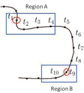
For example, Figure 3 shows a trajectory sequence and it includes fourteen points. The transformation result will
be 00AAAA0000BB00, where 0 indicates that this point
is not within any region. Although this trajectory sequence passes through Region A four times, it will be recorded once. Meanwhile, the trajectory points that are not within popular regions will be ignored. Furthermore, the trajectory may stay at a region for a while, but only the entry time will be taken into account. In other words, the trajectory in Figure 3 will be transformed into the region sequence RA
t1−t9
→ RB. When the
above step completes, the original trajectory sequence could be approximated by the region sequence.
C. Frequent Sequential Pattern Mining
When the region sequences are obtained, Algorithm 1 (Mod-ified PrefixSpan Algorithm), which is based on PrefixSpan [1] algorithm, is employed to extract frequent sequential patterns. In Algorithm 1, DatabaseScan procedure will get frequent 1-itemsets. For example, if we have four transactions as shown in Table I. After DatabaseScan procedure applying to the above sequences with the minimum support of value three, the frequent 1-itemset of the database will be a, b and d. A queue will be created to store these frequent items. Database
TABLE II PROJECTIONRESULT Transaction ID Sequence 1 b c d e 2 b c d 4 b
3
Algorithm 1 Modified PrefixSpan Algorithm
Input: A database DB with transaction list, minimum support min supp Output: Maximal Frequent List
1: 1-itemsetList← DatabaseScan(DB,min supp)
2: Queue← CreateQueue(1-itemsetList)
3: while Queue is not empty do
4: e← Queue.dequeue()
5: projectedItemList← DatabaseScan(Projection(e, DB), mini supp)
6: if projectedItemList is empty then
7: OUTPUT e
8: else
9: for all i such that1 ≤ i ≤ projectedItemList.Length do
10: Queue.enqueue(e.concat(projectedItemList[i])
11: end for
12: end if
13: end while
projection will be applied to the elements in the queue. For example, the first element in queue is a and Table II shows the result of a-projection on the database.
For each projection result, DatabaseScan procedure could be applied to get the frequent 1-itemset of the projected database and the projection item could combine the new itemset to obtain larger itemset. For example, the frequent 1-itemset in Table II is b, and it means that ab will be frequent itemset too and ab will be added into the queue for further process. When the above process is completed, the system could obtain frequent region patterns.
D. Bayesian Network Construction
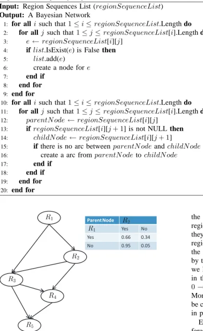
As mentioned above, frequent patterns on region sequences could be discovered by sequential pattern mining. The ana-lyzers could determine the regions they are interested in and the system could choose the patterns including these regions. These popular regions will be used to denote the random variables of the Bayesian network. In this paper, we assign each region an unique serial number. For example, if we are interested in Region1 − 5, and the frequent region sequences including these five regions are listed as follows:
R1→ R2→ R3→ R4
R2→ R4→ R5
R1→ R2→ R3→ R5
R2→ R3→ R4
R1→ R3→ R5
For each region sequence, we could construct a correspond-ing traversal path and Figure 4 shows the result. The ordercorrespond-ing of regions in the sequence indicates the visiting ordering, and the ordering is used to represent causal relationship of the Bayesian network. When the system processes R1 → R2 →
R3→ R4 sequence, a traversal path starting from R1 will be
constructed.
Essentially, a Bayesian network represents a system of probabilistic events as nodes in a directed acyclic graph. For the graphs with loops, it is possible to use loopy belief
propagation approach to approximate inference. However, be-cause the graph now has cycles, information can flow many times around the graph. For some models, the algorithm will converge, whereas for others it will not [9]. Meanwhile, in many applications such as tour planning and transportation routing analysis, people rarely re-visit the same place during a fixed time interval and cycle conditions in the trajectory sequence could be ignored. Thus, The region sequences with cycle condition will be removed in this paper. The construction of a Bayesian network structure using region sequences is presented in Algorithm 2, where Line1−9 will create a region node if this region node has not been created and Line10 − 20 will create the arc between parent node and child node.
In addition to the structure construction, we could construct the conditional probability table for each random variable from empirical data. In trajectory analysis, we define all the nodes as discrete-valued, where “Yes” and “No” are used to denote whether the moving objects have visited or not. As shown in Figure 4, the conditional probability table for node R1 will need to take into account two conditions: the
proportion of region sequences includes R1and the proportion
of region sequences does not pass through R1. According to
the empirical sequence data, the number of paths including R1
is 3, so the proportion would be 60%; while the proportion
of paths not including R1 is 40%. As for R2, it has one
parent node R1, so it has to take into account both its parent
node. The conditional probability table of R2 is presented in
Figure 4, where smoothing method is adopted to avoid the zero probability problem. Therefore, when the above processes are completed, we could construct a Bayesian network with structure and parameters.
IV. EXPERIMENT
In Bayesian network, inference is the process of updating probabilities of outcomes based upon the relationships in the model and the evidence known about the situation at hand. Therefore, performing inference means manipulating evidence in a model and obtaining the posterior probabilities resulting from the changes in evidence. Essentially, exact and approxi-mate inferences in Bayesian network is NP-hard, but we can
4
Algorithm 2 Trajectory Bayesian Network Construction Input: Region Sequences List (regionSequenceList) Output: A Bayesian Network
1: for all i such that1 ≤ i ≤ regionSequenceList.Length do
2: for all j such that1 ≤ j ≤ regionSequenceList[i].Length do
3: e← regionSequenceList[i][j]
4: if list.IsExist(e) is False then
5: list.add(e)
6: create a node for e
7: end if
8: end for
9: end for
10: for all i such that1 ≤ i ≤ regionSequenceList.Length do
11: for all j such that1 ≤ j ≤ regionSequenceList[i].Length do
12: parentN ode← regionSequenceList[i][j]
13: if regionSequenceList[i][j+ 1] is not NULL then
14: childN ode← regionSequenceList[i][j + 1]
15: if there is no arc between parentN ode and childN ode then
16: create a arc from parentN ode to childN ode
17: end if 18: end if 19: end for 20: end for Parent Node Yes No Yes 0.66 0.34 No 0.95 0.05
Fig. 4. Bayesian Network Structure for Region Sequences
nonetheless come up with approximations which often work well in practice. In our experiments, inference is performed by using MSBNx [10], which is a component-centric toolkit for modeling and inference with Bayesian network. MSBNx uses clique-tree propagation methods to calculate the probabilities and it provides an extensive programming interface that makes editing and evaluation of Bayesian Networks especially easy from COM-friendly languages such as Visual Basic, Jscript, and C#.
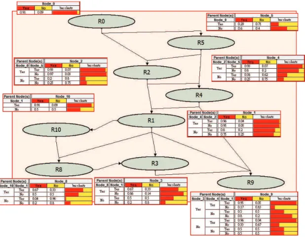
We use the trajectory data collected from GPS recorders to construct the Bayesian network. In the data set, there are 232 trajectory sequences. These trajectory sequences will be used to extract popular regions and the number of popular regions is 17. As mentioned above, the trajectory sequences does not pass through any popular region will be ignored and
the number of trajectory sequences passing through popular regions is 120. In practice, people could choose the regions they are interested in to perform the inference. We select 9 regions to construct the Bayesian network and Figure 5 shows the model result. The direction of arcs could be determined by the ordering of the regions in the sequences. For example, we have sequences <0, 2, 4, 1, 3, 9 > and < 0, 5, 2, 1, 3, 9 > in the raw data, so we could construct two traversal paths: 0 → 2 → 4 → 1 → 3 → 9 and 0 → 5 → 2 → 1 → 3 → 9. Moreover, the conditional probability table for each node could be constructed based on empirical sequence data as mentioned in previous section and they are presented in Figure 5.
Essentially, Bayesian network allows us to perform in-ference and get the probabilities of all possible states of an unobserved node under the current observed data. For example, when we have an evidence saying that the user’s current location is at R2, the system could further inference
user’s previous region is at R0 with a higher probability:
P r(R0= 1|R2= 1) = P r(R0= 1, R2= 1) P r(R2= 1) = 0.98 P r(R5= 1|R2= 1) = P r(R5= 1, R2= 1) P r(R2= 1) = 0.29 Besides, we could also derive possible reasons with a given cause. For example, when the user’s current location is at R0,
the system could obtain the probability of arriving at R1 is
0.93 and the probability of arriving at R8 is0.07. In general,
a Bayesian network could be designed to represent the deep causal knowledge of a domain expert and provide probabilistic answers to many queries by computing the posterior
probabil-5
Fig. 5. Trajectory Bayesian Network Experiment
ities over query nodes X, given the evidence E encountered so far.
V. CONCLUSION
In this paper, we proposed a novel approach based on Bayesian network to predict a moving object’s future location under uncertainty. Meanwhile, we proposed several algorithms to construct a Bayesian network from the trajectory informa-tion. The approach includes space-partitioning schemes, pop-ular region extraction, transformation of trajectory sequence and region sequence, frequent sequential pattern mining and the Bayesian network construction. The system allows the analyzers to determine the regions they would like to analyze and the system would retrieve all the frequent region patterns that include these regions. The transformation between the frequent region patterns and the Bayesian network includes two phases. The first phase is about the Bayesian network structure construction, where each popular region is regarded as a random variable in the Bayesian network. Meanwhile, the arcs between nodes of the Bayesian network are determined by the traversal paths of the frequent region patterns. In the second phase, the local probability distribution could be obtained based on empirical data. The experiment shows that the Bayesian network allows us to perform inference and get the probabilities of all possible states of an unobserved node under the current observed data.
ACKNOWLEDGMENT
This work was supported in part by the National Science Council under the Grants 97-2221-E-009-135 and NSC-97-2811-E-009-019.
REFERENCES
[1] J. Pei, J. Han, B. Mortazavi-Asl, and H. Pinto, “Prefixspan: Mining sequential patterns efficiently by prefix-projected pattern growth,” in
ICDE 2001, 2001, pp. 215–225.
[2] M. J. Zaki, “Spade: An efficient algorithm for mining frequent se-quences,” Machine Learning, vol. 42, no. 1, pp. 31–60, 2001. [3] F. Giannotti, M. Nanni, D. Pedreschi, and F. Pinelli, “Mining sequences
with temporal annotations,” in SAC ’06: Proceedings of the 2006 ACM
symposium on Applied computing, 2006, pp. 593–597.
[4] F. Giannotti, M. Nanni, F. Pinelli, and D. Pedreschi, “Trajectory pattern mining,” in KDD ’07: Proceedings of the 13th ACM SIGKDD
interna-tional conference on Knowledge discovery and data mining, 2007, pp.
330–339.
[5] H. Jeung, Q. Liu, H. T. Shen, and X. Zhou, “A hybrid prediction model for moving objects,” in The 24th International Conference on Data
Engineering, 2008, 2008, pp. 70–79.
[6] Y. Ishikawa, Y. Tsukamoto, and H. Kitagawa, “Extracting mobility statistics from indexed spatio-temporal datasets,” in STDBM, 2004, pp. 9–16.
[7] H. Jeung, H. T. Shen, and X. Zhou, “Mining trajectory patterns using hidden markov models,” in DaWaK 2007, 2007, pp. 470–480. [8] J. Pearl, Probabilistic Reasoning in Intelligent Systems: Networks of
Plausible Inference. Morgan Kaufmann, 1988.
[9] C. M. Bishop, Pattern Recognition and Machine Learning. Springer, 2007.
[10] C. Kadie, D. Hovel, and E. Horvitz, “MSBNx: A component-centric toolkit for modeling and inference with bayesian networks,” Microsoft Research Technical Report MSR-TR-2001-67, Tech. Rep., 2001.
98 年度專題研究計畫研究成果彙整表
計畫主持人:李嘉晃 計畫編號: 98-2221-E-009-141-計畫名稱:非監督式中文寫作自動評閱系統之研究與設計 量化 成果項目 實際已達成 數(被接受 或已發表) 預期總達成 數(含實際已 達成數) 本計畫實 際貢獻百 分比 單位 備 註 ( 質 化 說 明:如 數 個 計 畫 共 同 成 果、成 果 列 為 該 期 刊 之 封 面 故 事 ... 等) 期刊論文 0 0 100% 研究報告/技術報告 0 0 100% 研討會論文 0 0 100% 篇 論文著作 專書 0 0 100% 申請中件數 0 0 100% 專利 已獲得件數 0 0 100% 件 件數 0 0 100% 件 技術移轉 權利金 0 0 100% 千元 碩士生 4 4 100% 博士生 0 0 100% 博士後研究員 1 1 100% 國內 參與計畫人力 (本國籍) 專任助理 0 0 100% 人次 期刊論文 3 3 100% 研究報告/技術報告 0 0 100% 研討會論文 2 2 100% 篇 論文著作 專書 0 0 100% 章/本 申請中件數 0 0 100% 專利 已獲得件數 0 0 100% 件 件數 0 0 100% 件 技術移轉 權利金 0 0 100% 千元 碩士生 0 0 100% 博士生 0 0 100% 博士後研究員 0 0 100% 國外 參與計畫人力 (外國籍) 專任助理 0 0 100% 人次其他成果
(
無法以量化表達之成 果如辦理學術活動、獲 得獎項、重要國際合 作、研究成果國際影響 力及其他協助產業技 術發展之具體效益事 項等,請以文字敘述填 列。)除了三篇期刊論文 (IEEE Intelligent Systems 一篇,Expert Systems with Applications 兩篇),兩篇 Conference 論文 (ISICA 2008 與 ICNC'10 )之 外,目前尚有兩篇期刊論文分別於 Information Processing &; Management 與 IEEE Trans. on SMC -Part C 2nd revision 中。
成果項目 量化 名稱或內容性質簡述 測驗工具(含質性與量性) 0 課程/模組 0 電腦及網路系統或工具 0 教材 0 舉辦之活動/競賽 0 研討會/工作坊 0 電子報、網站 0 科 教 處 計 畫 加 填 項 目 計畫成果推廣之參與(閱聽)人數 0
國科會補助專題研究計畫成果報告自評表
請就研究內容與原計畫相符程度、達成預期目標情況、研究成果之學術或應用價
值(簡要敘述成果所代表之意義、價值、影響或進一步發展之可能性)
、是否適
合在學術期刊發表或申請專利、主要發現或其他有關價值等,作一綜合評估。
1. 請就研究內容與原計畫相符程度、達成預期目標情況作一綜合評估
■達成目標
□未達成目標(請說明,以 100 字為限)
□實驗失敗
□因故實驗中斷
□其他原因
說明:
2. 研究成果在學術期刊發表或申請專利等情形:
論文:■已發表 □未發表之文稿 □撰寫中 □無
專利:□已獲得 □申請中 ■無
技轉:□已技轉 □洽談中 ■無
其他:(以 100 字為限)
3. 請依學術成就、技術創新、社會影響等方面,評估研究成果之學術或應用價
值(簡要敘述成果所代表之意義、價值、影響或進一步發展之可能性)(以
500 字為限)
在本論文中,我們所提出的中文寫作多面向評分系統,有別於以往的評分系統,本系統將 不再需要事前訓練資料,且不再是以單面向、主觀的方式來給予評分,我們希望在評分上 能達到更高的可信度,因此提出了針對多面向來進行評分的方式,根據文章的結構、詞語… 等特徵,將各分數加以統整,在上述的實驗中,利用此方法所得之正確率達到 94.2%,證 明了多面向整合的評分方式較為客觀,且其實驗結果之整合分數比傳統的評分系統更足以 採信;此外,針對錯別字與各特徵都將給予回饋,使用者可藉由此回饋資訊得知在寫作上 有哪些需要改進的部份,以提升寫作能力。目前成果部分,有一篇論文已經被 IEEE Intelligent Systems 期刊接受, 兩篇論文被 Expert Systems with Applications 期刊接受,另外在決策樹方面我們提出一個簡化多 值化決策樹的方法,該論文已經被 ISICA 2008 接受,該論文也將會收錄於 LNCS 期刊; 另外尚有一篇論文被 ICNC'10 Conference 接受並且已經刊出。