On the complexity of search algorithms

1172 IEEE TRANSACTIONS ON COMPUTERS, VOL. 41, NO. 9, SEPTEMBER 1992

Foresight-Ok(n,constrained,curr)

Tentatively schedule n in the current instruction, curr. If there is a conflict, return FALSE. Update absolute times (tentatively).

Order constrained by minimum absolute time, ties are broken by maximum absolute time. For each m E constrained

Place m in the earliest instruction allowable. return(can all elements of constrained be placed?)

Fig. 6. Foresight-Ok algorithm.

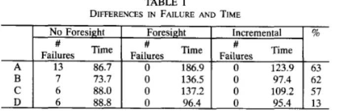
TABLE I

DIFFERENCES IN FAILURE AND TIME

Failures Time Failures Time Failures Time

73.7 136.5 97.4 62

C 6 88.0 0 137.2 109.2 57

D 6 88.8 0 96.4 0 95.4 13

using the foresight algorithm is 62.8 units, while the excess time of using the incremental algorithm is only 23.7 units, so the excess time saved by using the incremental is 62% ((62.8 - 23.7)/62.8).

The need for incremental compaction grows with the number of

[9] B. Su, S. Ding, J . Wang, and J. Xia, “Microcode compaction with timing constraints,” in Proc. 20th Microprogramming Workshop (MICRO-20), Colorado Springs, CO, Dec. 1987, pp. 59-68.

[lo] V. H. Allan and R. A. Mueller, “Compaction with general synchronous timing,” IEEE Trans. S o w a r e Eng., vol. 14, no. 5, pp. 595-599, May 1988.

[ l l ] H. F. Smith, Data Structures Form and Function. San Diego, C A Harcourt Brace Jovanovich, 1987.

[12] V. H. Allan, “A critical analysis of the global optimization problem for horizontal microcode,” Ph.D. dissertation, Comput. Sci. Dep., Colorado State Univ., Fort Collins, CO 80523, 1986.

[13] P. Wijaya, “Incremental foresighted microcode compaction,” Master’s thesis, Utah State Univ., Logan, UT, 1990.

[14] P. Wijaya and V. H. Allan, “Incremental foresighted local compaction,” in Proc. 22th Microprogramming Workshop (MICRO-22), Dublin, Ire- land, Aug. 1989.

finite maximum arcs. Overall, the incremental algorithm saves around 48% of excess time, and neither algorithm fails in compacting the examples. However, since this is still an increase over no foresight, it is better to use the incremental foresight algorithm only when the

DPS fails.

On the Complexity of Search Algorithms

Kuo-Liang Chung, Wen-Chin Chen, and Femg-Ching Lin 111. CONCLUSIONS

Compaction with timing constraints requires new techniques. Fore- sighted compaction is very effective in reducing failure inherent in

Abstract4onsider the average complexity for searching a record in a sorted file of records that are stored on a tape. We analyze in this note the

-

a greedy compaction algorithm. Incremental foresighted compaction

when discriminating compaction fails.

average complexity of four search algorithms, namely, sequential search, search. Our theoretical results are consistent with the recent simulation results bv Nishihara and Nishino. These results show that seauential reduces the cost to tolerable levels, but even then should only be used binary Fibonacci search, and a modified version Of Fibonacci

search, fibonacci search, and modified Fibonacci search are ali better than binary search on a tape.

Index Tems-complexity, Fibonacci search, generating function, mod- search*

REFERENCES

[l] J. A. Fisher, D. Landskov, and B. D. Shriver, “Microcode compaction: Looking backward and looking forward,” in Proc. Nut. Comput. Con$, vol. 50, Montvale, NJ, July 1981. M I P S Press, pp. 95-102. 121 D. Landskov, S. Davidson, B. D. Shriver. and P. W. Mallett, “Local

ified Fibonacci search’

I. INTRODUCTION

_ _

microcode compaction techniques,” ACM Comput. Surveys, vol. 12, no. 3, pp. 261-294, Sept. 1980.

[3] T. Nakatani and K. Ebcioglu, “Using a lookahead window in compaction-based parallelzing compiler,” in Proc. 23rd Microprogram- ming Workshop (MICR0-23), Orlando, FL, Nov. 1990.

[4] U. Banejee, S. Shen, D. J. Kuck, and R. A. Towle, “Time and parallel processor bounds for fortran-like loops,” IEEE Trans. Comput., vol.

C-28, no. 9, pp. 660-670, Sept. 1979.

[5] S. R. Vegdahl, “Local code generation and compaction in optimizing microcode compilers,” Ph.D. dissertation, Dep. Comput. Sci., Carnegie- Mellon Univ., Pittsburgh, PA, 1982.

[6] K. V. Palem and B. B. Simons, “Scheduling time-critical instructions on risc machines,” in Proc. Seventeenth Annu. ACM Symp. Principles Programming Languages, Jan. 1990, pp. 270-280.

[7] A. Aiken and A. Nicolau, “Optimal loop parallelization,” in Proc. SIG- P D W ’88 Con$ Programming Language Design and Implementation, Atlanta, GA, June 1988, pp. 308-317.

[8] A. Nicolau and R. Postasman, “An environment for the development of microcode for pipelined architectures,” in Proc. 23rd Symp. and Workshop Microprogramming and Microarchitecture, Orlando, FL, Nov. 1990, pp. 69-79.

Consider a search key and a sorted file of records stored on a tape. The goal of a search algorithm is to find the record saved on the tape that matches the given key.

In this note we investigate the average complexity of four known search algorithms, namely, sequential search (SS), binary search (BS),

Fibonacci search (FS), and a modified version of Fibonacci search (mFS). For the purpose of analyzing the complexity of these four search algorithms, we shall only concern the average total distance that the reading head is required to move for searching a record. This Manuscript received September 21, 1990; revised October 6, 1991. This work was supported in part by the National Science Council of R.O.C. under Grant NSC79-0408-E002-07.

K.-L. Chung is with the Department of Information Management, National Taiwan Institute of Technology, Taipei, Taiwan 10772, R.O.C.

W.-C. Chen and F.-C. Lin are with the Department of Computer Science and Information Engineering, National Taiwan University, Taipei, Taiwan 10764, R.O.C.

IEEE Log Number 9103107.

IEEE TRANSACTIONS ON COMPUTERS, VOL. 41, NO. 9, SEPTEMBER 1992

is due to the fact that moving the reading head of the tape takes much longer time than reading and comparing the current record with the search key. Hence, head movement time, which is proportional to the traveling distance, is the dominant factor in the search time.

To make the complexity analysis easier, we shall assume that the sorted file containing F,, - 1 records, where F,, is the nth Fibonacci number. Our main results derived in Section I11 show that the complexities of SS, BS, FS, and mFS are asymptotically equal to

O..IF,, , F,,

,

0.882F7,, and 0.809F,, , respectively. Our results indicate that algorithm SS is optimal and gives 30% better efficiency than BS; mFS gives 19.1% better efficiency than BS; and FS is 11.8%

better than BS. Some of these results are consistent with the recent simulation results by Nishihara and Nishino [4].

11. THE PERFORMANCE EQUATIONS

This section first describes the basic concepts of the BS, FS,

and mFS algorithms and then derives their corresponding recurrence equations for the average complexity formulas (complexity, for short). The recurrence equations for the average distance of the head movement required by the algorithms for external search on a tape were derived recently in [4]. However, they did not solve the recurrence equations to get the closed forms of the formulas. Instead, they used these recurrence equations iteratively to obtain the approximate performance values for some specific file sizes. In this note we solve the recurrence equations to get the closed forms of the formulas. These formulas are then used to compare the search complexities of the four search algorithms.

With the BS algorithm described in [3], we begin a search process by comparing the search key with the record in the middle of the sorted file. The orbit of BS on the sorted file consists of a root node containing a record and the links to the left and right subtrees which are defined in the same way. The left subtree contains those keys which are smaller than the key at the root, whereas the right subtree contains the larger keys in comparison with the root. Given, say, 12 records

IC1

.

I<z. . . . .IC12 and the search key I<, the first record being examined is IC6 which is labeled by the index 6. If l i e is less than

IC, then IiS is examined; otherwise l i 3 is examined. Continuing this process, the binary tree with root at level 0 describing this process is shown in Fig. l(a) and the search sequences with only the first three probes on the storage are shown in Fig. l(b).

In order to make the analysis easier, we may assume that the number of records in the sorted file is F,, - 1 = 2"' - 1 for some

I I I

2

1 . We also assume that each record is searched with equal

probability. Under these assumptions, the complexity of BS is given by

21(2'''-t - 1)

1

/(F,t - 1). (1)

T B . s ( I ~ ) =

(

2"'-'-'

O < >

<,,!

- 1

The reading mechanism moves 2"'-'-' units of length when travers- ing a node at level ( i - 1) to a node at level i . Therefore, the time needed in a search step is 2"'-'-'. The number of subtrees whose roots are at level i is 2' and the size of those subtrees is 2'n-1 - 1 . Furthermore, each node in the corresponding subtree accumulates

2"'- 1 - c

An alternative method proposed by Ferguson [ l ] is FS which splits the file according to the Fibonacci sequence. The Fibonacci sequence is defined as

time units when one search step is passed.

F(, = 0. F I = 1.

F, = Ft-,

+

Ft--2 for i

2

2.

In FS, we first examine the F,,-znd record instead of the middle one. The F,,-and record corresponds to the root of the Fibonacci

1173

(a)

1st

2nd a d

(b)

Fig. 1 . (a) A binary search tree. (b) Search sequences of BS.

1st

A A

1 2 3 4 5 6 7 8 9 1 0 1 1 12

a d 2nd

(b)

Fig. 2. (a) A Fibonacci search tree. (b) Search sequences of FS.

tree containing F,, - 1 nodes. Based on the comparison result, we then (recursively) search either the left subtree or the right subtree which contains F,,-Z - 1 or Fn-l - 1 records. For example, given 1 2

records (TI = 7), the Fibonacci tree describing the splitting process

is shown in Fig. 2(a), and the search sequences of FS with the first three probes are shown in Fig. 2(b).

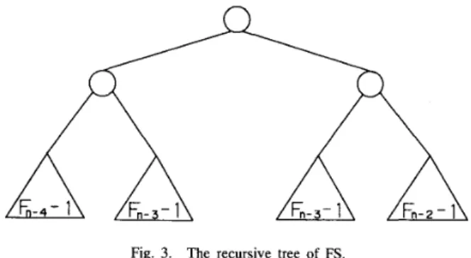
Consequently, the total search time is equal to F,L-2(FrI - 1) plus the total amount of time needed in the left and right subtrees. As shown in Fig. 3, the distances from the root of the original tree to the roots of the left and right subtrees are both Fn-3. In fact, for any node, the distance from this node to its two subtrees are equal. However, since the splitting point is decided by the Fibonacci

1174 IEEE TRANSACTIONS ON COMPUTERS, VOL. 41, NO. 9, SEPTEMBER 1992

Fig. 3. The recursive tree of FS.

sequence, the sizes of these two subtrees are different, namely,

Fn-2 - 1 for the left subtree and Fn-l - 1 for the right subtree. Thus, the complexity of FS is T ~ s ( n ) = pn-z/(Fn - l), where

pn is subject to

pn = F n ( F n + 2 - 1 ) + p n - l + Qn-1,

qn = Fn(Fn+l - 1)

+

pn-2

+

qn-2 for 7~

2

2 ( 2 ) with the initial conditions p o = 0, p l = 1, qo = 0, and 41 = 0 [4]. Note that the initial condition can be obtained by checking the case n = 4.

A modified version of FS (mFS) is proposed to keep the amount of head movement as small as possible [4]. In FS, the sizes of the splitted pair of subfiles (subtrees) always form the two numbers F, - 1 and

F,+1- 1. In mFS, while the moving manner of the reading mechanism is similar to that of FS, the splitting position is decided such that the splitted part with smaller length F, always abuts the current position of the reading head. The probe sequence defined in this way can keep the head movement small since the reading mechanism moves only

F, units of length in each search step.

The modified Fibonacci tree describing the splitting process is shown in Fig. 4(a) and the search sequences of mFS with the first three probes are shown in Fig. 4(b). The complexity of mFS, which can be derived by virtue of Fig. 5, is equal to T , F s ( ~ ) =

sn-2/(Fn - l), where s n is subject to recurrence

s, =

Fn(F,+2

- 1 )

+

s , - ~

+

sn-z for n

2

2 ( 3 )

with initial values SO = 0 and s 1 = 1 [4].

111. THE ANALYSIS OF COMPLEXITIES

In this section, we analyze the complexities of SS, BS, mFS, and FS. First, the complexities of SS and BS can be analyzed rather easily.

Theorem 1: The complexity of SS is Tss(n) M 0.5Fn. Proof: In SS, the complexity T s s ( n ) is given by

M 0.5Fn. This completes the proof.

Theorem 2: The complexity of BS is TBS ( n ) M F,,

.

Proof: Replacing the term 2" in (1) by F,, we have

T B S ( n ) =

(

2"-1-z22"(2m-t - l ) ) / ( F n - 1) O < z < m - l F, - 1 M- (2"(2" - 1 ) - m2"-') "N F,.

I

Fig. 4. (a). A modified Fibonacci search tree. (b) Search sequences of mFS.

n

Fig. 5. The recursive tree of mFS.

Before analyzing the complexities of mFS and FS, we need some important lemmas and corollary. The following three lemmas are from [2].

Lemma 1: Fn+, = Fm-lFn

+

Fn+lFm.

Lemma 2:

where M 1.618 and

4

M -0.618. Lemma 3:

From Lemma 1-afd the fact that Fn+l M 1.618Fn [2], we obtain

Corollary 1: F2,, M 2.236FnFn.

Theorem 3: The complexity of mFS is T , ~ s ( n ) M 0.809Fn.

F k F n - k = 9 F n

+

F F n - 1 .

the following corollary.

Proof: Since T , ~ s ( n ) = sn-2/(Fn - l), we first solve s n - 2

in (3) as follows:

st = Fz(Fz+2 - I )

+

sz--l

+

s,-2 for i

1:

2, where SO = 0 and s1 = 1.

Taking the generating function on both sides of the above equation, we have

S ( 3 ) = 3

+

z S ( z )

+

Z 2 S ( 3 )

+

C F Z ( F 2 + 2 - l)ZZ

IEEE TRANSACTIONS ON COMPUTERS, VOL. 41, NO. 9, SEPTEMBER 1992 1175

where S ( z ) =

as shown in

[2].

right-hand side of (4), thus

s , z z and G ( z ) = 2 / ( 1 - z

-

2 ' ) =

Cz2"

F,zz

The value of s n P 2 is equal to the coefficient of tn-' on the -

S n - 2 = FkFn-k-lFvz-k+l -

E

FkFn-n-i.

OSk<n-l 0 5 k < , I - 1

From Lemma 3, the above equation is

n - 2 2n

-

2

Fn-2. ( 5 )

Fn-1 -

-

Then using Lemma 2 and Corollary 1, we can calculate the

_ -

summation term in the right-hand side of (5).

FkFn-k--IFn-k+i OSkSn-1 - + J n + l Q n - k - l + Q n - I d n - k + l - - - + 4 k d 2 n - 2 k - J k 4 2 n - Z k

JZn-,,.

( 6 )

Although, there are 8 summation terms in the right-hand side of (6),

only the following two terms need be considered:

M 5.854F2, M 13.090FnFn, J k 4 2 , 1 - 2 k - -

(in

-

d 2 n ) @ 2

O < k L n - l

4

- d2 M l.81Fzn % 4.047Fn F,. (7)

The other 6 summation terms can be ignored because their values are too small to affect the analytical result. For example, the fourth term is

% 0.691Fr3,

which is quite small, compared with the above hvo summation terms. Plugging the right-hand sides of (7) into (6), we have

FkFn-k--lFn-k+l M 0.809FnF,,. ( 8 )

O<k<n-l

Finally, from ( 5 ) and (8) we get

~ ~ % -0.809FnFn. 2

Thus, T , F S ( I I ) = S , - L ) / ( F ~ ~

-

1 ) % 0.809F7,.

I

Theorem 4: The complexity of FS is T F S ( n ) M 0.882F,,. Proof: Since

T ~ s ( n )

= pn-2/(F,, - l ) , we first solve p n - 2 in (2) as follows:

p t = Ft(F,+z - 1) +p,-i

+

~ ~ - 1 :

qL = Ft(FL+l - 1) +pl--2 +q,--2 for i

2

2 where PO = 0 , p l = 1,yo = 0 , and q1 = 0.

equations and obtain

We take the generating function on both sides of the above

P ( z ) = z

+

IP(z)

+

z Q ( z )

+

F,(FL+2 - l) z ' , (9)

1>2

Q ( Z ) = Z ~ P ( Z )

+

2~(.)

+

C

F , ( F , + ~ -

6 2 2

where P ( z ) = C 1 > O p L z *

,

Q ( z ) =

Cz20qztz.

Replacing Q ( z ) in (9) by the right-haid side of (lo), we have

P ( z ) = 2

+

2 P ( _ , )

+

-

(a(_.)

1 - 22 1

-

2 2

+

C F z ( F z + 2 - 1 ) ; ' ) -- - - - ,2 ( 2

+

A

E

FC(FL+l -

1b'

1 2 2 L>2 = ( 1 - z 2 ) G ( z )

+

G ( 3 ) F,(F,+1 - 1 ) z ' 222 1 -

+

+G(z) Ft(Fz+z

-

1 ) ~ ' L >2 = G ( z ) F,(F,+1 - 1 ) ~ '

+

( 1 - z 2 ) G ( z ) &>0

.

C

F , ( F , + ~ - ~ ) ~ ' - l . (11) * > O

The value of p n - 2 is the coefficient of z n P 2 in the right-hand side

of (ll), thus

P n - 2 %

1

FkFn-k-2Fn-k-1 O < k < n - 2

-

c

FkFtt-k--3F~~-k--l- (12)

OSk<n-3

Each summation term in the right-hand side of (12) is similar to the term in (11) and thus can be calculated using Lemma 2 and Corollary 1 as follows: FkFn--l;--2Fn-k-1 0.085F2, M 0.191FnFn. O < _ k < n - 2 FkFn--k--lFn-k+l % 0.362F2, % 0.809FnFn. FkFn-k-3Fn-k-1 NN 0.053F2, M 0.118FnFn. O < k < n - 1 O < k < n - - 3

Substituting the values of the above summation terms into (12), we have

p n - 2 M 0.882FnF,,.

1176

IV. CONCLUSIONS

Theorems 1 and 2 give

TSS/TBS

N 0.5. That is, SS is 50% better than BS. Theorems 2 and 3 give T,,,b \/TB\ M 0.809, or

mFS is 19.1% more efficient than BS. Theorems 2 and 4 give

TFS/TBS

z 0.882 or FS is 11.8% more efficient than BS. In

summary, when searching on a tape, sequential search, Fibonacci search, and modified Fibonacci search are all better than binary search. Moreover, modified Fibonacci search indeed is better than Fibonacci search.

In [4], Nishihara and Nishino wrote computer programs to eval- uate the performance values by iteratively applying the recurrence equations in Section 11. When the size of the sorted file is more than 2000 records, they obtained the approximate efficiency ratios as

TFS/TBS

z 0.882 and

Tm~s/T&

N 0.809. These experimental values confirm our theoretic results derived in this note.

REFERENCES

D. E. Ferguson, “Fibonacci searching,” Commun. ACM, vol. 3, no. 12, pp. 648, 1960.

D. E. Knuth, The Art of Computer Programming, Vol. I , Fundamental Algorithms, 2nd ed.

D. E. Knuth, The Art of Computer Programming, Vol. 3, Sorting and Searching. Reading, M A Addison-Wesley, 1973.

S. Nishihara and H. Nishino, “Binary search revisited: Another advan- tage of Fibonacci search,” IEEE Trans. Comput., vol. C-36, no. 9, pp.

Reading, MA: Addison-Wesley, 1973.

1132-1135, 1987.

Exact Parametric Analysis

of Stochastic Petri Nets

Man Li and Nicolas D. Georganas

Abstract- An algorithm for exact parametric analysis of Stochastic

Petri Nets is presented. The algorithm is derived from the theory of Decomposition and Aggregation of Markov Chains. The transition rate of interest is confined into a diagonal submatrix of the associated Markov Chain by row and column permutations. Every time a new value is assigned to the transition, a smaller Markov Chain is analyzed. As a result, the computational cost is greatly reduced.

Index Terms-Decomposition and Aggregation, Markov Chain, para- metric analysis, stochastic Petri Nets.

1. INTRODUCTION

Stochastic Petri Nets, introduced independently by Molloy [6] and Natkin [7], are a tool for modeling systems with concurrency, synchronization, and communication. They have been widely used in the performance analysis of communication systems, protocols, manufacturing systems, etc.

Manuscript received July 25, 1990; revised April 24, 1991. This work was supported in part by the Natural Science and Engineering Research Council

of Canada under Grant A-8450 and the Ontario University Research Incentive Fund under Grant OT9-003.

The authors are with the Department of Electrical Engineering, University

of Ottawa, Ottawa, Ont., Canada K1N 6N5. IEEE Log Number 9103109.

IEEE TRANSACTIONS ON COMPUTERS, VOL. 41, NO. 9, SEPTEMBER 1992

According to Molloy [6], the continuous time Stochastic Petri Net is defined as

S P S = ( P . T . 3. R )

P = { p ~ , p ~ : . . p ~ , } is a set of places

T = { t ~ . f z ; . . f , ~ } is a set of transitions A

c

{ P x

T}

U { T x P }

R = { r l , r q , .

. .

T , , ~ } is a set of firing rates for the exponentially distributed transition firing times.

Molloy further showed that any finite place, finite transition, marked Stochastic Petri Net is isomorphic to a Markov Chain. As a result, the usual way of analyzing a Stochastic Petri Net is to generate the Reachability Graph (RG) of the Stochastic Petri Net and at the same time construct the associated Markov Chain. The markings constitute the states of the Markov Chain (hence we will use “state” and “marking” alternatively) and the transition rates between markings constitute the infinitesimal generator matrix. Solving the Markov Chain, we obtain the steady-state probabilities. From these probabilities, we obtain the performance measures of interest.

Frequently, in the performance analysis by Stochastic Petri Nets, we are interested in the behavior of the system with respect to one parameter, or one transition. By assigning different values to this transition, we may obtain the effect of this particular transition on the whole system performance. One drawback of this analysis is that every time the transition rate is changed, we have to analyze the whole net again. This is a tedious procedure. Regarding this problem, Ammar [l] recently proposed a time scale decomposition method for analyzing a kind of Stochastic Petri Net whose transition rates differ by orders of magnitude. Approximate results were obtained. Li and Georganas [5] proposed the parametric analysis of a class of Stochastic Petri Nets whose underlying Markov Chain satisfies local balance equations. They showed that exact results can be obtained in an approach analogous to Norton’s theorem. Both [l] and [5] dealt with only a special class of Stochastic Petri Nets. In this paper, w e propose exact parametric analysis of Stochastic Petri Nets in general. The idea is based on the theory of Decomposition and Aggregation of Markov Chains.

The organization of this paper is as follows: Section I1 gives an introduction to decomposition and aggregation techniques and then derives an algorithm for parametric analysis. Section I11 considers the computational gain achieved by the algorithm compared with directly solving the Markov Chain by Gaussian elimination. Section IV deals with implementation of the algorithm to parametric analysis of Stochastic Petri Nets. Section V gives an example and Section VI concludes this paper.

11. EXACT PARAMETRIC ANALYSIS OF STOCHASTIC PETRI NETS We give an introduction to decomposition and aggregation tech- niques and then derive an algorithm for parametric analysis.

A. The T h e o v of Decomposition and Aggregation

The decomposition and aggregation techniques were first proposed by Simon and Ando [9] in the early 1960’s. The primary feature of the decomposition and aggregation techniques is reducing the analysis of a large system into that of a set of smaller problems.

Let Q be the infinitesimal generator matrix of a continuous time Markov Chain. Assume Q is an rt x t t matrix. Q is partitioned into