An exemplar-based learning model for hydrosystems prediction and categorization

(1)

ELSEVIER

Journal

Journal of Hydrology 169 (1995) 229-241 141

An exemplar-based learning model for hydrosystems

prediction and categorization

Fi-John Chang*, Li Chen

Department of Agricultural Engineering, National Taiwan University. I, Sec. 4, Roosevelt Rd.. Taipei, 10770, Taiwan

Received 8 February 1994; accepted 7 September 1994

Abstract

The main purpose of this paper is to represent a new Exemplar-Based Learning model and to apply this model for river flow estimation. The central idea of the model is based on a theory of learning from examples. This idea is similar to human intelligence: when people encounter new situations, they often explain them by remembering old experiences and adapting them to fit. To explore the stability and efficiency of the model performance, a simple mathematical function is simulated by the model. The model is then applied to extend the annual stream flow records according to the nearby stream flow stations and to classify the monthly flow by using the monthly rainfall and runoff information in the previous months. The results show that the model has better performance than the traditional methods and the results demonstrate the power and efficiency of the model for the hydrological data analysis.

1. Introduction

Natural phenomena are marvellously complex and varied, and events never repeat exactly. But even though events are never the same, they are also not completely different. There is a thread of similarity and continuity, so we are able to predict from past experience to future events. Although natural phenomena in general do not have well-defined rules or fixed boundaries separating alternatives, most early work in model fitting used well-defined concepts, such as regression analysis or hypothesis testing theories. Focusing on such issues has the relative difficulty of acquiring different rules, strategies for testing alternative hypothesis, and the transfer of behavior to new stimulus sets.

* Corresponding author.

(2)

230 F.-J. Chang, L. Chen / Journal of Hydrology 169 (1995) 229-241

Owing to recent technological advances in computer-aided design, it is now much easier to build massively parallel machines. This has contributed to a new wave of interest in models of computation that are inspired by neural nets rather than the formal manipulation of symbolic expressions. The exemplar-based learning (EBL) algorithm is one of the new trends in that domain. The EBL is a very powerful method for category formation, especially in complex real-world situations where complete causal information is not available. The basic idea of this algorithm is based on a theory of learning from examples. This idea is similar to much of human intelligence. When people encounter a new situation, they often explain it by remembering old experiences and adapting them to fit.

In this paper we describe the nested hyper-rectangles learning model (Salzberg, 1988, 1989, 1991) which is based on the EBL algorithm (Medin and Schaffer, 1978; Schank and Leake, 1989; Minton et al., 1989). Next, we explore the stability and efficiency by using the nested hyper-rectangles learning model to: (1) simulate a simple mathematical function; (2) extend the short record stream flow; (3) classify the monthly flow. We then conclude by comparing the results from the nested hyper- rectangles learning model with traditional approaches.

2. Major characteristics of the exemplar-aided constructor of hyper-rectangles (EACH)

The strategy of the exemplar-based learning (EBL) algorithm is based on storing points (or examples) in Euclidean n-space, F’, where it is the number of variables or features in an example, then comparing the new example to those, and finding the most similar example in memory. The algorithm is a very powerful tool for prediction or categorization tasks. The EACH, proposed by Salzberg (1989), is a new theory of EBL where the points in the EBL are generalized into hyper-rectangles. As the generalizations grow large, there may exist some exceptions which create ‘holes’ in the hyper-rectangles. These may in turn give holes inside them, resulting in a nested structure of hyper-rectangles.

To show the powerfulness and usefulness of the EACH, several important characteristics summarized from Salzberg (1989) are described below.

2.1. Knowledge representation schemes

Many systems acquire rules during their learning processes; however, these rules do not exhaust the possible representation of the knowledge that learning may acquire. EACH, on the other hand, creates a memory space filled with exemplars, some of which represent generalizations; and some of which represent individual examples from the system’s experience.

2.2. Learning strategies

Incremental and non-incremental learning are two main strategies used by machine learning systems (Michalski et al., 1983). The main shortcoming of non-incremental

(3)

F.-J. Chang, L. Chen 1 Journal

of

Hydrology 169 11995) 229-241 231 strategies is inefficiency; for example, to insert a new example, the entire set of previous examples must be added to build a model. EACH is an incremental learning strategy in which systems model with each example they process; however, it also has a disadvantage in that it is sensitive to the order of the inputs. As stated by Salzberg (1991) the problem of creating an optimal number of rectangles to classify a set of points is NP-hard, consequently the problem can not be solved in polynomial time now.

2.3. One-shot learning

A machine learning system capable of one-shot learning should be able to learn a new concept or category from one example. Some learning models rely on notions of statistics which make one-shot learning very difficult. Some systems require that statistical outliers be confirmed by additional examples before they can be used in category formation. In EACH, once a new point has been stored in memory, which may occur after a single example, it is immediately available for use in prediction.

2.4. Discrete and continuous variables

EACH can handle variables that are binary, discrete, and/or continuous. For continuous variables, the model has an error tolerance parameter, which indicates how close two values must be in order to be treated as ‘match’; consequently, the continuous variables are approximated by a discrete set of values.

2.5. Disjunctive concepts

Many concept learning programs have ignored disjunctive concepts because they are more difficult to learn than conjuncts. EACH handles disjunctions very easily in its structured exemplar memory. It can store many distinct exemplars which carry the same category label. A new example which matches any one of these distinct exemplars will fall into the category they represent. A set of such exemplars represents a disjunctive concept definition.

Salzberg (1989) used the EACH on three different domains: predicting the recur- rence of breast cancer, classifying iris flowers, and predicting survival times for heart attack patients. In all cases, he demonstrated that EACH performs as well as, or better than, other algorithms which were run with the same data sets.

3. The nested generalized exemplar learning algorithm

The basic algorithm of EACH is that it uses some existing events as a foundation to predict the outcomes of other events by building the structure of hyper-rectangles. This process includes adjusting the weights of the model’s parameters in time and making the system learn. The main procedures are described as below.

(4)

232 F.-J. Chang, L. Chen / Journal of Hydrology 169 (1995) 229-241

3.1. Initial work

For the sake of making predictions, EACH must have a history of examples as the bases of its predictions. Consequently, the first step is to seed some examples which are randomly chosen from the training set. This process simply stores each selected example in memory without attempting to make any predictions. An example, in fact, is a vector of features, where each feature may have any number of values, ranging from 2 (for binary variables) to infinity (for real valued). According to Salzberg (1991), the number of seeds was determined by trial and error on a simulated data set, and performance was insensitive to the size of the seed set.

3.2. Match and classify

After initialization, every new example is matched to memory by a matching process. This process uses the distance metric to measure the distance (or similarity) between a new data point (an example) and an exemplar (an existing point or hyper-rectangle in _I?). The best match is the one which has the smallest distance and is then used to make a prediction in the way that the new example has the same category as the closest matching exemplar.

Let the new example be E and the existing hyper-rectangle be H. The match score between E and His calculated by measuring the Euclidean distance between the two objects. The distance is determined as follows:

Let HI,~,~

be the lower end of the range, and Hupper be the upper end, then the distance metric becomes

{

Efi - Hupper when & > Upper & - Hri = HI,,,, - Eri when Eri < HI,,,

0 otherwise

The distance measured by this formula is equivalent to the length of a line dropped perpendicularly from the point Efi to the nearest surface, edge, or corner of H. Note that points internal to a hyper-rectangle have distance 0 to that rectangle.

Where Wh is the weight of the exemplar H, Wi is the weight of the feature i, Efi is the value of the ith feature in example E, Hfi is the value of the ith feature in exemplar H, mini, maxi are the minimum and maximum values of that feature, and m is the number of features.

The formula divides distances along each dimension by (maxi - mini) in order to standardize them to the interval [O,l] so that each feature in the exemplars has the same basis.

There are two weights in the distance metric, W,, and Wi. W, is a simple measure of how frequently the exemplar, H, has been used to make a correct prediction. W, is the ratio of the number of times H has been used to the number of times it has resulted in

(5)

F.-J. Chang, L. Chen / Journal of Hydrology 169 (1995) 229-241 233 a correct prediction. Consequently, it can indicate the reliability of each exemplar. Thus if a hyper-rectangle His used many times, but nearly always makes the wrong prediction, the weight W,, will grow very large, and H will tend not to be chosen as the closest match in the future. If H is a noisy point, then it will eventually be ignored as

W, increases. The minimum value of W,, is unity in the case of perfect prediction. The other weight measure, Wi, is the weight of the ith feature. These weights are adjusted to reflect the fact that all features do not normally have equal importance in a category decision.

3.3. Feedback

EACH adjusts the weights Wi on the feature fi after discovering that it has made the wrong prediction. Weight adjustment is executed in a very simple loop: for each fi if & matches Hfi, the weight Wi is increased by setting Wi = Wi( 1 + Af), where Af is the global feature adjustment rate. An increase in weight causes the two objects to seem farther apart; if Efi does not match Hfi, then W, is decreased by setting Wi = Wi(l - Af).

3.4. The procedures of EACH

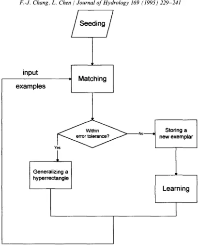
Fig. 1 is the flow chart of the EACH algorithm. The procedure is summarized as follows.

(1) Seeding: EACH uses historical examples to predict events in the future. (2) Matching: use a distance metric. Each new example is matched to the exemplar in the memory with the minimum distance score.

(3) Feedback:

(a) if the system makes a correct prediction, then a new hyper-rectangle is generalized;

(b) if the system makes a wrong prediction, then the new example E is taken as a single point and stored in the memory.

(4) Learning: When the system makes a mistake, EACH can automatically adjust each Wi in the following way:

(a) if any Efi is too close to Hfi, then Wi is set to Wi(l + Af); (b) if any Efi is not close to Hfj, then Wi is set to Wi(l - Af).

3.5. Explanation of paradigm

Fig. 2 shows the geometric picture of the seeding and matching processes for the case of two variables.

Let function: Y = 3 Xl + 2 X2 and error tolerance = 6 Given: three training data = (2, 1; S), (3, 2 ; 13), (1, 7; 17) Find: two predicting data = (5, 6; Y,r), (2, 2; Y,,)

(6)

234 F.-J. Chang. L. Chen 1 Journal of Hydrology 169 (1995) 229-241 input examples . b Matching

FA

Within storing a error tolerance? NO Yes _-cl new exemplar

1

Generalizing a hyperrectangle . Learning 1. Training:

(0)

(1)

(2)

Fig. 1. The flow chart of the EACH algorithm.

seeding one point:

input: Hl (2, l), YH1 = 8 memorize one point [(2, 1); 81 adding one point

input: El (3, 2), YEI = 13

calculate: DEIHl = [(3 - 2)* + (2 - 1)2]o.5 = 1.414 error = (YE1 - YE21 = 113 - 81 = 5 < 6 execute: construct a hyper-rectangle Hl

memorize: a hyper-rectangle [(2,1), (3,2); 81 adding another point

input: E2 (1, 7), YE2 = 17

calculate: DE2H1 = [( 1 - 2)* + (7 - 2)2]o.5 = 5.099 error=IYE2--YHII=117-81=9>6

execute: store a single point E2

(7)

F.-J. Chang. L. Chen 1 Journal of Hydrology 169 (1995) 229-241 235 . x2 E2 P2 El Pl a 1 2 3 4 5 6 7 8 Xl Fig. 2. The geometric picture for the EACH. 2. Predicting:

(1)

(2)

Pl ( 5,6 ), Ypl = ? input: (5, 6)

calculate: DPIHl = [(5 - 3)’ + (6 - 2)2]o.5 = 4.472 DPIE2 = [(5 - l)* + (6 - 7)2]o.5 = 4.123 execute: match point E2

set Ypl = YE2 = 17 (true value of Ypl = 20) P2 (2, 2) Yp* = ?

input: (2, 2)

calculate: DPZH1 = 0 (P2 within hyper-rectangle H2) DP2n2 = [(2 - l)* + (2 - 7)2]o.5 = 5.099 execute: match hyper-rectangle Hl

set Yp2 = Yn, = 8 (true value of Yp2 = 10)

4. Tests, results and discussions

4.1. Theoretical case

Stability and efficiency are two important factors when one deals with model performance. To show the general characteristics of the EACH performance, a simple mathematical function,

Y = Xl2 +X22 (O<Xl,X2< 1)

(8)

236 Table 1

F.-J. Chang, L. Chen 1 Journal of Hydrology 169 (1995) 229-241

Relationship between the number of hyper-rectangles and predictive accuracy The number of

hyper-rectangles

Mean (%) Standard deviation (%)

5 55.94 15.02

10 78.00 11.29

15 85.72 8.59

20 90.78 5.58

25 94.45 2.72

predict the dependent variable Y. First, an n set of (Xl, X2, Y) is randomly selected as input data for EACH. The function has two random variables, Xl and X2, so the distance metric is two dimensions. The error tolerance is set as 0.2; i.e. if the difference between the forecasting value and true value is within 0.2, it is considered as a ‘match’ and is set in the same hyper-rectangle. The procedure then is run with all the 12 data set to build up the nested hyper-rectangles in the E2 domain.

After the training task is completed, the EACH model’s performance is then estimated. It begins with randomly selected N new sets of (Xl, X2), then uses the set model, without modifying or changing the model structure or parameters, to predict Y values and compare the predicted values with true values from the mathematical function. If the error is within 0.2, the forecast result is accounted as correct; otherwise it is incorrect. In order to determine the effect of the number of nested hyper-rectangles, m, to the prediction accuracy, we test several different numbers of m, i.e. m = 5,10,15,20,25. In each case, 100 sets of (X1,X2) were performed to match their Y values by using the EACH model with a different number of nested hyper-rectangles in the model, and the number of correct times were recorded. The procedures were run 100 times for the purpose of statistical analysis.

The results are shown in the Table 1. We found that as ‘m’ increases, the mean value of the correct times will increase and the standard deviation will decrease. The results support the concept that when we have more experiences, we are more sophisticated.

4.2. Stream flow extension

Stream flow records have been extensively used in a wide variety of water resources studies. Unfortunately, we often face the problem that the records of stream flow are too short to contain a sufficient range of hydrological conditions or have periods of missing data. To solve this problem, we may transfer information from nearby stream gages, that is, use the historic records and extend them in time by the correlation between flow at the site of interest and concurrent flow at nearby gage(s) (Alley and Burns, 1983). However, if the correlation is low, extending the records by using such a method directly would be questionable.

The nested hyper-rectangles algorithm provides a feasible alternative in this cir- cumstance. In the following, we used four stream flow gages in the Potomac basin, USA to demonstrate the usefulness of the algorithm for annual stream flow extension.

(9)

Table 2

F.-J. Chang, L. Chen 1 Journal of Hydrology 169 (1995) 229-241 237

Mean annual flow in c.f.s. at the Strausburg, Antietam, Point of Rocks and Cumberland stations (1931- 1960)

Strausburg (Sl) Antietam (S2) Point of Rocks (S3) Cumberland (S4) 282 158 4642 731 675 309 10100 1314 344 268 7767 1192 325 268 7056 1344 804 242 11350 1649 330 127 4665 643 742 383 10840 1237 741 479 11010 1336 745 423 13030 1609 500 278 8543 1231 1047 378 13210 1440 490 228 7867 1228 241 192 5220 750 592 257 8828 1172 567 231 8925 1439 366 181 6849 1134 998 357 13480 1652 461 242 6144 986 430 270 7317 1087 545 280 9108 1175 610 251 9002 1113 494 209 8692 1218 769 336 12670 1574 984 340 13440 1570 767 251 10670 1356 226 173 4856 760 790 344 12700 1480 378 168 6920 1060 232 125 4920 852 402 229 6490 799

The data of annual stream flows from 1931 to 1960 were obtained from Salas et al. (1980) and are shown in Table 2. For each case, one station was taken as having a short-record gage so that its last 10 years’ annual flow needed to be estimated and the other three stations were taken as having a long-record. The first 20 years of concurrent annual flow of the short-record gage and the long-record gages were used as a training set to build up the EACH model. As the model is set, its structure and parameters would not be modified and it is used to predict directly the last 10 years’ stream flow for the short record gage by using the concurrent records from the other three gages. The error tolerance is set to 85 c.f,s. For comparison, the multiple linear regression is performed with the same data set for each case. The results are shown in Table 3. The mean absolute error of EACH is smaller than that of multiple regression even in the case where it has a very high correlation. Apparently, the EACH has better performance than the multiple regression.

(10)

238 F.-J. Chang, L. Chen / Journal of Hydrology I69 (1995) 229-241 Table 3

The mean absolute errors of four stations using EACH and multiple regression methods Names of station Hyper-rectangle

Strausburg (Sl) 58.7 Antietam (S2) 43.8 Point of Rocks (S3) 488.2 Cumberland (S4) 63.9 Linear regression 63.2 53.8 537.5 128.6 Years of training, N = 20; years of prediction, m = 10.

The function of linear regression and the coefficients of multiple determination: Sl = 1.153 - 0.69882 + 0.13S3 - 0.325S4, R2 = 0.9345; S2 = 56.339 - 0.39731 + 0.078S3 - 0.20484, R2 = 0.7517; S3 = -310.522 + 6.34381 + 6.716S2 + 3.05184, R2 = 0.9768; S4 = 268.44 - 1.14Sl - 1.25882 + 0.2233, R2 = 0.8488.

In the following it is shown how the number of training sets influences the prediction; the gage at Point of Rocks (S3) is used as a case study. The first 5, 10, 15 and 20 years of stream flow records are used to set up the EACH model. The model is then used to predict the last 10 years’ stream flows. The multiple linear regression is also performed by using the same data sets in each situation. The results are shown in Table 4.

The results are consistent with the theoretical case; that is, the model has better performance as the training data are increased. Also, the EACH has smaller mean absolute errors than the multiple regression in most of the cases, even the regression correlation is very high. Moreover, it is found that the mean absolute error in the linear regression case for N = 5 is 815, while for N = 10 it is 1030 and for N = 15 it is

Table 4

The results of station Point of Rocks (S3) as N = 5,10,15,20

Flows N=5 N= 10 N= 15 N = 20

Linear Hyper Linear Hypcr Linear Hyper Linear Hypcr 9002 8692 12670 13440 10670 4856 12700 6920 4920 6490 7717 8257 7767 12483 11350 12345 11350 9707 10100 4108 4642 11742 11350 6540 7761 4391 4642 4917 4642 10100 8019 8543 8007 8828 8640 8828 7194 8543 8303 7867 7943 7867 12841 13030 11663 13030 11626 13030 13207 11350 11479 13210 13004 13210 9390 10100 9368 10100 10377 10100 3631 4642 5312 5220 4604 5220 12640 13030 11148 13030 11526 13030 5129 7767 6977 7767 6449 6849 2728 4642 5346 5220 4600 5220 5621 4642 6009 4642 6215 4642

Mean absolute error 815 1054 1030 715 863 585 537 488

The function of linear regression: N = 5, S3 = -4119.914 - 0.67581 + 10.55832 + 8.62494; N = 10, S3 = -5199.247 + 1.26831+ 28.20582 + 4.82184; N = 15, S3 = -1115.325 - 0.94831+ 11.092S2 + 6.21434; N = 20, S3 = -310.522 + 6.34381 + 6.71632 + 3.05134.

(11)

F.-J. Chang, L. Chen / Journal of Hydrology 169 (1995) 229-241 239

863, i.e. the addition of 200% extra training points has worsened the performance of the linear regression method. This anomaly is due to small sample size and incon- sistent data structures within the training sets and predicting years.

4.3. Streamjlow forecasting

The final task in this series given to EACH was to classify/predict the average daily stream flow in April for 29 years at the Shihmen Reservoir, Taiwan. The data sets were obtained from Chang and Hsu (1990) and they also cover three different hydrological factors which may influence the stream flow in April: (1) the average daily stream flow; (2) the maximum daily stream flow; (3) the average daily rainfall in the. Each stream flow was classified as three levels as obtained from Chang and Hsu (1990). The level of stream flow (Y) was classified as follows. If:

(1) Y < 9 CMS then stream flow under average oil); (2) 9 < Y < 16 CMS then average condition (~2);

(3) 16 < Y < 50 CMS then stream flow above average (~3).

EACH seeded the 29 years’ records. After the training process, it established 12 hyper-rectangles and it could precisely predict the level of Y by using the three hydrological factors in the previous month (i.e. March). Comparing the optimal calibrated results obtained with Baye’s decision rules and fuzzy inference rules (with the same data set) obtained from Chang and Hsu (1990) showed that the correct prediction rates were 5 1.7% for Baye’s rules and 62.1% for fuzzy inference rules, while the EACH could make a perfect prediction. The fuzzy inference rules and EACH were also used to predict the average daily stream flow of April in 1986 and 1987, and both methods made a correct prediction. The results are shown in Table 5.

5. Conclusion

Three advantages of the nested hyper-rectangle learning model have been found. (1) Saving computer memory: similar types of data are categorized as a hyper- rectangle and only two diagonal points of each are memorized in its computing procedure, so the memory space can be reduced dramatically.

(2) Learning ability: the model can dynamically adjust its parameters through the feedback of new added examples. The model has the ability to learn. Consequently, the model will be more sophisticated for prediction and/or categorization if more examples (data) have been used on its training procedure.

(3) Fast execution: because the executing time is linear (not exponential) to the number of hyper-rectangles; so even if there are thousands of hyper-rectangles, the result can be obtained within a few seconds.

The model is applied to extend annual stream flows using the long records of nearby gage-stations. The results show that the model is better than the multiple linear regression method. In the case of classifying the monthly flow, the model

(12)

240 Table 5

F.-J. Chang, L. Chen / Journal of Hydrology 169 (1995) 229-241

Streamflow classification /prediction using three different methods Year 1957 1958 1959 1960 1961 1962 1963 1964 1965 1966 1967 1968 1969 1970 1971 1972 1973 1974 1975 1976 1977 1978 1979 1980 1981 1982 1983 1984 1985 Flow 17.3 9.4 17.2 12.7 11.8 22.6 5.6 6.1 6.7 9.4 7.0 26.7 8.3 12.5 8.2 10.0 15.5 24.5 22.0 8.7 4.6 33.0 14.4 10.3 8.8 9.7 36.8 22.1 31.0 Class Baye’s - Accuracy (X) Y3 Y2 Y2 Y2 Y3 YJ Y2 Y2 Y2 Y3 Y3 Yl YJ Yl Yl Yl Yl Yl Y2 Y2 Yl Yl Y3 Y3 YJ Y2 Y2 Y2 Yl Yl Y2 Yl Y2 YJ Y3 Y2 Y3 Y2 Yl Y2 Yl Yl Y3 Y3 Y2 Y2 Y2 Yl Yl Y2 Y2 Y3 Y3 Y3 Y3 Y2 Y3 Y3 51.7 Y3 Y2 Yl Yl Y3 Y3 Yl Yl Yl Y2 YJ Y3 Y2 Y3 Yl Yl Yl Y2 Y3 Yl Yl Y3 Y2 Y2 Y3 Y3 Y3 Y2 Y3 Fuzzy - 62.1 + + _ _ _ + + + + + + + - _ + _ _ _ + + + + + + _ _ + _ + her Y3 Y2 Y3 Y2 Y2 Y3 Yl Yl YJ Y2 Yl Y3 YJ Y2 Yl Y2 Y2 Y3 Y3 Yl Yl Y3 Y2 Y2 Yl Y2 Y3 Y3 Y3 100 + + + + + + + + + + + + + + + + + + + + + + + + + + + + + +, Correct classification/prediction. -, Incorrect classification/prediction.

does completely distinguish the investigated data set, while the rates of correct classification of Baye’s decision rules and fuzzy inference rules are 51.7% and 62.1%, respectively, which were obtained from Chang and Hsu (1990). The results demonstrate that the model is a very powerful and efficient tool for prediction and/or categorization in the field of hydrological data analysis.

References

Alley, W. M. and Burns, A. W., 1983. Mixed-station extension of monthly streamflow records. AXE J. Hydraul. Eng., 109(10): 1272-1284.

Chang, F.J. and Hsu., K.L., 1990. A study for streamflow forecast. J. Chin. Agric. Eng., 36(4): l-12. Medin, D. and Schaffer, M., 1978. Context theory of classification learning. Psychol. Rev., 85(3): 207-238.

(13)

F.-J. Chang, L. Chen / Journal of Hydrology 169 (1995) 229-241 241 Michalski, R., Carbonell, J. and Mitchell, T. (Editors), 1983. Machine Learning. Springer, Berlin. Minton, S., Carbonell, J.G., Knoblock, CA., Kuokka, D.R., Etzioni, 0. and Yolanda, G., 1989. Explana-

tion-based learning: a problem solving perspective. Artif. Intell., 40: 63-118.

Salas, J.D., Delleur, J.W. and Lane, W.L., 1980. Applied Modeling of Hydrologic Time Series. Water Resources, Littleton, CO.

Salzberg, S., 1988. Exemplar-based learning: theory and implementation. Tech. Rep. TR-10-88, Center for Research in Computing Technology, Harvard University.

Salzberg, S., 1989. Nested Hyper-Rectangles for Exemplar-Based Learning. In: J. Siekmann (Editor), Lecture Notes in Artificial Intelligence. Analogical and Inductive Inference. Int. Workshop A11’89, l-6 October 1989, Reinhardsbrunn Castle, GDR, Springer, pp. 184-201.

Salzberg, S., 1991. A nearest hyper-rectangle learning method. Mach. Learn., 6: 251-275.

Schank, R.C. and Leake, K.B., 1989. Creativity and learning in a case-based explainer. Artif. Intell., 40: 353-385.