人體動作辨識之推論與取樣頻率研究

國 立 交 通 大 學

電 控 工 程 研 究 所

碩 士 論 文

人體動作辨識之推論與取樣頻率研究

Inference and Down-sampling Rate study for

Video-based Human Action Recognition

研 究 生 ： 劉 育 誠

指 導 教 授： 張 志 永

人體動作辨識之推論與取樣頻率研究

Inference and Down-sampling Rate study for

Video-based Human Action Recognition

學 生 : 劉育誠 Student : Yu-Cheng Liu

指導教授 : 張志永 Advisor : Jyh-Yeong Chang

國立交通大學

電控工程研究所

碩士論文

A Thesis

Submitted to Department of Electrical Engineering

College of Electrical Engineering

National Chiao-Tung University

in Partial Fulfillment of the Requirements

for the Degree of Master in

Electrical and Control Engineering

July 2012

人體動作辨識之推論與取樣頻率研究

學生:劉育誠 指導教授: 張志永 博士

國立交通大學電機與控制工程研究所

摘要

人體動作辨識系統在電腦視覺領域一直是很熱門的研究與應用目標。在居家 監控系統中最常見的方式是，使用固定式的攝影機，對室內的人物進行追蹤與動 作辨識。為了達到即時監控之目標，處理的演算法必須快速，而且又必須能夠有 效的分析影像。 在本論文中，動作辨識的目標是人體，為了更正確的擷取出人體部份，我們 同時使用灰階域與 HSV 色彩空間，建立兩個背景模型，提升消除影像中陰影部 分之影響，使得前後景之分離結果能夠更完整。取得即時影像，擷取出的前景部 份，經過特徵空間轉換與標準空間轉換後，累積三張動作影像後，藉由預先學習 而建立之模糊法則與時序動作姿態比對，完成人體動作之辨識。 研究對於較短周期的動作其取樣頻率改變是否獲得更多資訊，更多的訊息可 以使人體動作辨識更加的準確，並且對判斷相同動作的規則，取其最大或者前三 大、前五大、前七大和前九大相似度的動作法則平均值，藉由更多規則決定目前 輸入的影像與判別動作之間的相似度，確能更加準確判斷人體動作。

Inference and Down-sampling Rate study for

Video-based Human Action Recognition

STUDENT: Yu-Cheng Liu ADVISOR: Dr. Jyh-Yeong Chang

Institute of Electrical and Control Engineering National Chiao-Tung University

ABSTRACT

Human activity recognition system is now a very popular subject for research and application. Using a fixed camera to track a person and recognize his (her) activity is widely seen in home surveillance. For real-time surveillance, the embedded algorithms must be efficient and fast to meet the real-time constraint.

In the thesis, we build two background models, one is grayscale another is HSV color space that extract the human region correctly, and we also reduce the shadowing effect. For better efficiency, the binary image is transformed to a new space by eigenspace and canonical space transformation. After that, we gathered three consecutive down-sampled images to recognize the human actions by fuzzy rules.

We utilize different down-sampling rate for short-period action to obtain more information which is useful for the human action recognition. Furthermore, we investigate to the average value of maximal top-3, top-5, top-7 and top-9 firing strength of rules with the same action to recognize the human action. Using more rules to determine the similarity between the inputs and rules that can be more accurately determine human action.

Acknowledgment

I would like to express my sincere gratitude to my advisor, Dr. Jyh-Yeong Chang for valuable suggestions, guidance, support and inspiration he provided. Without his advice, it is impossible to complete this research. Thanks are also given to all the people who assisted me in completing this research.

Finally, I would like to express my deepest gratitude to my family for their concern, supports and encouragements.

Contents

摘要 ...………..………...i

ABSTRACT ……….……….…...ii

Acknowledgment………...………..iii

Contents ………...iv

List of Figures ………vii

List of Tables ………..……….ix

Chapter 1 Introduction ………1

1.1 Motivation of this research ………...………1

1.2 Foreground extraction ………..………4

1.3 Eigenspace and Canonical Space Transformation ………….……...………5

1.4 Image Frame Classification and Activity Recognition ………….…………6

1.5 Thesis Outline ………..………7

Chapter 2 Basic Concept ………8

2.1 Fundamentals of Eigenspace and Canonical Space Transform ………8

2.1.1 Eigenspace Transformation (EST) ..………10

2.2 The HSV color space ..………14

Chapter 3 Human Activity Recognition System ….………17

3.1 Object Extraction ………17

3.1.1. Background Model ….……….17

A. Grayscale Value Background Model………..…17

B. HSV Color Space Background Model……….18

3.1.2. Foreground Object Extraction………..………19

3.1.3. Shadow Suppression ………...………22

3.1.4. Object Segmentation ………...………24

3.1.5. Foreground Image Compensation ………...………24

3.2 Background Update ………27

3.3 Down-sampling the Video Stream …...………..29

3.4 Construction of Fuzzy Rules from Video Stream………...33

3.5 Classification Algorithm……….37

Chapter 4 Experimental Results ...39

4.3 The Recognition Rate of Activities ………50

Chapter 5 Conclusion ……….63

List of Figures

Fig. 1.1 Block diagram showing the human action recognition system…....………….3

Fig. 2.1 The HSV Cone. ……….………...……..14

Fig. 3.1 The framework we apply to foreground subject extraction.……..………….20

Fig. 3.2 The binary image is projected on X-axis and Y-axis..………26

Fig. 3.3 The binary image of extracted foreground region.……….………26

Fig. 3.4 The walking video sequences..……….………..…29

Fig. 3.5 The jog video sequences……….….………..…… 29

Fig. 3.6 The running video sequences………30

Fig. 3.7 Using 5:1 down-sampling rate to select the essential template images.……30

Fig. 3.8 Common states of two different activities………33

Fig. 3.9A fuzzy rule learned to classify action………... 36

Fig. 3.10 Utilizing the average value of maximal top-3 firing strength.…………... 38

Fig. 4.1 One of the environment in our LAB databases.……….………39

Fig. 4.2 Another environment in our LAB databases.………..39

Fig. 4.3 An example of hand region extraction. (a) Weizmann databases (b) KTH databases………...40

Fig. 4.3 An example of hand region extraction. (c) LAB databases...41

Fig. 4.4 Showing an example of foreground extraction. (a) Background image. (b) Input image. (c) Grayscale value image. (d) Binary image. (e) Extraction foreground image...43

Fig. 4.5 Some essential templates use the same down-sampling rate. From top to bottom: walking, jog and running, respectively……….44

Fig. 4.7 30 essential templates for Weizmann databases…...………46 Fig. 4.8 20 essential templates for KTH databases.……….…47 Fig. 4.9 30 essential templates for our LAB databases.………….………..48 Fig. 4.10 The statistic velocity of walking, jog and running from the KTH dataset……….…..51 Fig. 4.11 Normalizing the statistic velocity.………..………..51

List of Tables

Table I Some of the Obtained Fuzzy Rule Base………..50 Table II Action Recognition Use 5:1 Down-Sampling Rate on KTH dataset…….…52 Table III Action Recognition Use 5:1 for Walking, 3:1 for Jog and 2:1 for Running Sampling Rate………..………52 Table IV Action Recognition Use 5:1 for Walking, 3:1 for Jog and 2:1 for Running Sampling Rate with Velocity factor………..53 Table V Action Recognition Use the Maximum Firing Strength on Weizmann databases………...…………54 Table VI Action Recognition Use the Average Value of maximal Top-3 Firing Strength on Weizmann databases……….54 Table VII Action Recognition Use the Average Value of maximal Top-5 Firing Strength on Weizmann databases……….55 Table VIII Action Recognition Use the Average Value of maximal Top-7 Firing Strength on Weizmann databases……….56 Table IX Action Recognition Use the Average Value of maximal Top-9 Firing Strength on Weizmann databases……….56 Table X Action Recognition Use the Maximum Firing Strength on KTH databases...57 Table XI Action Recognition Use the Average Value of maximal Top-3 Firing Strength on KTH databases………..…57 Table XII Action Recognition Use the Average Value of maximal Top-5 Firing Strength on KTH databases………..…58

Table XIV Action Recognition Use the Average Value of maximal Top-9 Firing Strength on KTH databases………..…58 Table XV Action Recognition Use the Maximum Firing Strength on LAB databases………..………….59 Table XVI Action Recognition Use the Average Value of maximal Top-3 Firing Strength on LAB databases………..…60 Table XVII Action Recognition Use the Average Value of maximal Top-5 Firing Strength on LAB databases………..…60 Table XVIII Action Recognition Use the Average Value of maximal Top-7 Firing Strength on LAB databases………..…61 Table XIX Action Recognition Use the Average Value of maximal Top-9 Firing Strength on LAB databases………..…62

Chapter 1 Introduction

1.1 Motivation of this research

Recognizing human actions in monocular video is an important scene understanding issue for applications [1] such as automatic surveillance, content-based video search, human-computer interaction, intelligent environment, and many others. Our society is becoming increasingly aging. Thus, home nursing is getting more and more important. However, the price of most home nursing care service is very expensive. Besides, the trained nurses are limited and they cannot take care of the elderly 24 hours a day. Therefore, automatic home caring system plays an important role to this trend. For example, when automatic surveillance system recognizes one's human activity is dangerous, the alarm will be triggered. Nevertheless, there is no well-defined structure which is effective to recognize the human actions to data. Therefore, this makes human action recognition become a challenging task.

A number of human action recognition methods have been proposed in the past few years. Carlsson and Sullivan et al. [6] proposed an action recognition method by shape matching to key frames from edge data which obtained from canny edge detection. Luke and Keller et al. [5] utilized using fuzzy logic to model human activities from voxel person. Cohen and Li [4] presented a 3D visual-hull constructed from a set of silhouettes to infer the human postures. W4 [2] can detect single person or several persons in group by using an adaptive background model and identify the activities by finding the body components on the silhouette boundary. Bobick et al. [3], recognized human activities by comparing motion's energy and history.

In our research, we have designed a robust method that makes use of shape features to recognize the human actions. It is know that, when people do a specific action, which are composed of similar posture sequences in the time axis. Therefore, we can down-sample the frame sequence to recognize the human actions. Then, we use the 5:1, 3:1 and 2:1 down-sampling rate to classify the three consecutive key postures and then use the maximum, the average value of maximal top 3, top 5, top7 and top 9 firing of the action rule to recognize the human action.

The human action recognition system is composed of three modules. The first module is foreground extraction. The second module is the posture classification module which will transform the image data to a smaller dimension for computational and storage efficiency. Then the foreground image will be classified to the key postures of actions. The third module is the inference module which reasons the using the fuzzy rules to classify the three consecutive posture sequences to recognize the human action. The human action recognition system is showing in Fig. 1.1.

Input frame image Background image Background model Foreground detection Foreground image EST CST

Inference from three consecutive posture

sequences

Learned action fuzzy rule base Three posture

sequence

The first module

The second module

The third module

1.2 Foreground extraction

The foreground subject extraction is the first step of human action recognition. We need to construct a background model. Background subtraction is a method typically used to segment moving regions in image sequences taken from a static camera by comparing each new frame to a model of the scene background [7]. There are many methods to build background models. In Piccardi [8], a review of the most relevant background subtraction methods were presented. W4 [2] is such a popular example that using frame-difference with a threshold. In addition, foreground subject extraction is commonly affected by the additional inclusion of shadows. A lot of attempts have been developed to tackle the shadow suppression. Horprasert et al. [9] and Cucchiara et al. [10] utilized the rationale that shadows have similar chromaticity, but lower brightness than the background model. In our system, we build two background models. The first one is based on grayscale value and the second is based on HSV color space. In short, the background model should be adoptive to the represent the scene change. A subject enters scene and then leaves some things in the scene. After the subject leaves the scene, the background model will be updating accordingly.

After building the background model, we can extract the foreground subject from video frames. Subtracting each pixel of background model from current image frames will produce foreground subject. Then, the resulting image is converted to a binary image which contains the foreground subject by setting a threshold. Therefore, we can extract the most possible region of a person to a rectangle binary image. The rectangle image is resized to the specified resolution for normalization.

1.3 Eigenspace and Canonical Space Transformation

In most of video and image processing, the size of frame is usually very large and it usually contains a great deal of redundancy. The redundancy wastes the resources greatly in computation and storage aspects. Hence, some space transformations are introduced to reduce the redundancy of an image by reducing the data size of the image. The first step of redundancy reduction often transforms an image from a high-dimensional space into a low-dimension space. The transformation can use fewer dimensions to approximate the original image. There are many well-known transformation methods such as Fourier Transformation, Wavelet Transformation, Principal Component Analysis, Multi Dimensional Scaling (MDS) and Locally Linear Embedding (LLE). Our transformation method combines eigenspace transformation and canonical space transformation which are described as follows.

The Eigenspace Transformation (EST), which is based on Principal Component Analysis (PCA), has been demonstrated to be a potent scheme used for automatic face recognition [11], [12], gait analysis [13] and action recognition [14]. The subsequent transformation, Canonical Space Transformation (CST) based on Canonical Analysis, is used to reduce data dimensionality and to optimize the class separability and improve the classification performance. Unfortunately, CST approach needs long computation efforts when the image is large. Therefore, we combine EST and CST in order to improve the classification performance while reducing the dimension. Thus each image can be projected from a high-dimensional spatiotemporal space to a low-dimensional canonical space. In this low-dimension space the recognition of

1.4 Image Frame Classification and Activity Recognition

In this thesis, images are transformed into an image feature vector by extracting features from images. We extract image features by using eigenspace transformation and canonical space transformation. Because of the cameras usually capture image frames with a frequency of 30 frames per second. There is not much difference between two consecutive image frames. Thus, down-sampling the input image stream is necessary and that can reduce the computation load and complexity.We group three contiguous down-sampled images and transform them to three consecutive feature vectors. Then, the time-sequential images are converted to a posture sequence by using these three feature vectors. The posture sequence is signified by the number of the templates. In the learning phase, we build a transition model in terms of three consecutive posture sequences which are the category symbol of the posture template. For human action recognition, the model which best matches the observed posture sequence is chosen as the recognized action category.

One of the famous methods to model the time-sequential data's transition model is Hidden Markov Models (HMMs). The basic concept of Hidden Markov Models is described in [15]. HMMs have been used in speech recognition [16] and hand gestures recognition [17]. After transforming image frames to eigenspace and canonical space domain, we greatly reduce the image data size. We adopt the fuzzy rule-based techniques to classify human activities, not by the shape-based features of the images. Therefore our activity analysis system is tolerant of dissimilarity, uncertainty, ambiguity and irregularity which exist in the action video. Relevant articles using the fuzzy theory in action recognition are described as follows. Wang and Mendel [18] proposed that fuzzy rules to be generated by learning from examples.

Su [19] presented a fuzzy rule-based approach to spatio-temporal hand gesture recognition.

In our system, we propose a fuzzy rule-base approach for human activity recognition. Each action is represented in the form of fuzzy IF-THEN rules, extracted from the posture sequences of the training data. Each IF-THEN rule is fuzzified by employing an innovative membership function in order to represent the degree of the similarity between a time-based three posture pattern and the corresponding antecedent to infer the subject's action. When our system classifies an unknown action video, we match the three contiguous down-sampled images to the precedent part of each fuzzy rule. The rule's consequent with maximal accumulated similarity measure associated with these three consecutive postures defines the subject's activity type.

1.5 Thesis Outline

The thesis is organized as follows. In Chapter 2, we introduce the basic concepts concerning eigenspace transform, canonical space transform, and the HSV color space. In Chapter 3, we describe that utilizing different down-sampling rate to select the key postures and investigating to the average value of maximal top-3, top-5, top-7 and top-9 firing strength of rules with the same action to recognize the human action. In Chapter 4, the experiment results of our recognition systems are shown. At last, we conclude this thesis with a discussion in Chapter 5.

Chapter 2 Basic Concept

In this chapter, we briefly explain the basic concepts of eigenspace and canonical space transform. Then HSV color space concept is introduced.

2.1 Fundamentals of Eigenspace and Canonical Space

Transform

In video and image processing, the dimensions of image data are often extremely large. It is common to transform the image from high-dimensional space into a low-dimension one to discover a small set of composite features for action recognition. There are many well-known transformation methods such as Fourier Transformation, Wavelet Transformation, Principal Component Analysis (PCA), Multi Dimensional Scaling (MDS) and Eigenspace Transformation (EST). However, PCA based on the global covariance matrix of the full set of image data is not very effective to the class structure existent in the data. In order to enhance the discriminatory power of various activity features, Etemad and Chellappa [20] introduced Linear Discriminant Analysis (LDA), also called canonical analysis (CA) [21], which can be used to optimize the posture class separability of different activity classes and improve the classification performance. The features are obtained through maximizing between-class and minimizing within-class variations. Here we call this approach canonical space transformation (CST). To benefit from these two transforms, combining EST based on PCA and CST based on CA. Therefore, our approach reduces the data dimensionality and optimizes the posture class separability of different activity classes.

Image data in high-dimensional space are converted into low-dimensional eigenspace using EST. Then, the obtained vector is further projected to a smaller canonical space using CST. Action Recognition is accomplished in the canonical space.

Assume that there are c training classes to be learned. Each class represents a specific posture, which assumes of testers various forms existing in the training image data. x′ is the j-th image in class i, and Ni,j i is the number of images in the i-th class.

The total number of images in training set isNT =N1+N2++Nc. This training set

can be written as

[

x′1,1,,x1′,N1,,x′2,1,,x′c,Nc

]

(2.1)

where each x′ is an image with n pixels. i,j

At first, the intensity of each sample image is normalized by

. , , , j i j i j i x x x ′ ′ = (2.2)

Then, the mean pixel value for the training set is given by

1 . 1 1 , x

∑∑

= = = c i N j j i T i N x m (2.3)

The training set can be rewritten as an n×NT matrix X. And each image xi,j forms

a column of X, that is

2.1.1 Eigenspace Transformation (EST)

Basically EST is widely used to reduce the dimensionality of an input space by mapping the data from a correlated high-dimensional space to an uncorrelated low-dimensional space while maintaining the minimum mean-square error to avoid information loss. EST uses the eigenvalues and eigenvectors generated by the data covariance matrix to retain the original data coordinates along the directions of maximal variance sequentially.

If the rank of the matrix XXT is K, then K nonzero eigenvalues of XXT, λ1, λ2, ,λK, and their associated eigenvectors, e1,e2,,eK , satisfy the

fundamental relationship

λiei =Rei, i=1,2, ,K (2.5)

where T

XX

R= and R is a square, symmetric n× matrix. In order to solve n

Eq. (2.5), we need to calculate the eigenvalues and eigenvectors of the n× matrix n

T

XX . But the dimensionality of XX is the image size, it is usually too large to be T

computed easily. Based on singular value decomposition, we can get the eigenvalues and eigenvectors by computing the matrix R~ instead, that is

T

: =

R X X X data matrix (2.6)

in which the matrix size of R~ is NT ×NT which is much smaller than n× of R. n

Then the matrix R~ still has K nonzero eigenvalues K

~ , , ~ , ~ _{λ λ} λ1 2  and K associated eigenvectors ~e1,~e2,,~eK which are related to those in R by

( )

    λ = λ = λ − i i i i i e X e ~ ~ ~ 2 1 i = 1 , 2,,K (2.7)

These K eigenvectors are used as an orthogonal basis to span a new vector space. Each image can be projected to a point in this K-dimensional space. Based on the theory of PCA, each image can be approximated by taking only the largest eigenvalues λ₁ ≥ λ₂ ≥≥ λ_k , k ≤K , and their associated eigenvectors

k

e e

e1, 2,, . This partial set of k eigenvectors spans an eigenspace in which yi,j are

the points that are the projections of the original images xi,j by the equation

[

]

T

, , ,1 2 , , 1, 2,..., ; 1, 2,...,

i j = k i j i= c j= Nc

y e e  e x (2.8)

We called this matrix

[

e1,e2,,ek

]

T the eigenspace transformation matrix. After

this transformation, each image xi,jcan be approximated by the linear combination of

these k eigenvectors and yi,j is a one-dimensional vector with k elements which are

their associated coefficients.

2.1.2 Canonical Space Transformation (CST)

Based on canonical analysis in [22], we suppose that

{

φ1,φ2,,φc

}

represents

the classes of transformed vectors by eigenspace transformation and yi,j is the j-th

vector in class i. The mean vector of entire set can be written as

_y 1 _{i j,} 1, 2, , ; 1, 2, , _i i j T i c j N N =

∑∑

= = m y   (2.9)

The mean vector of the i-th class can be presented by 1 . Φ ,

∑

∈ = i i,j j i i i N y y m (2.10)

Let Sw denote the within-class matrix and Sb denote the between-class matrix,

then

(

)(

)

(

)(

)

∑

∑ ∑

= = ∈ − − = − − = c i y i y i i T c i i j i i j i T N N N _{ij i} 1 T 1 φ T , , 1 1 , m m m m S m y m y S y b w

where Sw represents the mean of within-class vectors distance and Sb represents the

mean of between-class distance vectors distance. The objective is to minimize Sw and

maximize Sb simultaneously, which is known as the generalized Fisher linear

discriminant function and is given by

( )

_T . T W S W W S W W J w b = (2.11)

The ratio of variances in the new space is maximized by the selection of feature transformation W if =0. ∂ ∂ W J (2.12)

Suppose that W* is the optimal solution where the column vector w is a *i

generated eigenvector corresponding to the i-th largest eigenvalues λ . According to i

After solving (2.11), we will obtain c–1 nonzero eigenvalues and their corresponding eigenvectors

[

v₁,v₂,,v_c−1

]

that create another orthogonal basis and span a (c–1)-dimensional canonical space. By using these bases, each point in eigenspace can be projected to another point in canonical space by

i j

[

c

]

i,j T 1 2 1 , v ,v , ,v y z =  − (2.14)

where z represents the new point and the orthogonal basis i,j

[

]

T 1 2

1,v , ,vc−

v  is

called the canonical space transformation matrix. By merging equation (2.8) and (2.14), each image can be projected into a point in the new (c－1)-dimensional space by

zi,j = Hxi,j. (2.15)

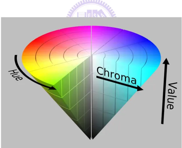
2.2 The HSV color space

The HSV (hue, saturation and value) color space corresponds closely to the human perception of color. Conceptually, the HSV color space is a cone as shown in Fig. 2.1. Viewed from the circular side of the cone, the hues are represented by the angle of each color in the cone relative to the 0o line, which is traditionally assigned to be red. The saturation is represent as the distance from the center of the circle. Highly saturation color are on the outer edge of the cone, whereas gray tones (which have no saturation) are at the very center. The value is determined by the colors vertical position in the cone.At the point end of the cone, there is no brightness, so all colors are blacks. At the fat end of the cone are the brightness colors.

The formula of RGB transfers to HSV is defined as below:                      = ° + − − × ° = ° + − − × ° < = ° + − − × ° ≥ = ° + − − × ° = ° = B max min max G R G max min max R B B G R max min max B G B G R max min max B G min max H if , 240 60 if , 120 60 and if , 360 60 and if , 0 60 if , 0     − = = otherwise , 0 if , 0 max min max max S max V = (2.16)

where max =max(R,G,B) and min=min(R,G,B).

The hue parameter is the value which represents color information without brightness. Therefore, the hue is not affected by change of the illumination brightness and direction. Although hue is the most useful attribute, there are three problems in using hue attribute for color segmentation: 1) hue is meaningless when the intensity value is very low, 2) hue is unstable when the saturation is very low, and 3) saturation is meaningless when the intensity value is very low [18]. Accordingly, Ohba et al.[23] use three criteria (intensity value, saturation, and hue) to obtain the hue value reliably.

 Intensity Threshold Value:

If V < , then V_t H =0, where V , V , and _t Hare an intensity value, the intensity threshold value, and a hue value, respectively. If measured color is not bright enough, the color is discarded. Then, the hue value is set to a predetermined value, i.e., 0.

 Saturation Threshold Value:

If S< , then St H =0, where S, S , and t Hare an saturation value, the

saturation threshold value, and a hue value, respectively. Using this equation, measured color close to gray is discarded in the image.

 Hue Threshold Value:

If 0<H <Ht or, 2π−Ht <H <2π then H =0. The range of hue

value is from 0 to 2π , and it has discontinuity at 0 and 2π . We use the phase

Chapter 3 Human Activity Recognition System

The first step of human activity recognition system is foreground subject extraction. We need to construct a background model. There are many well-known methods to build background models. The most common one is that applying frame difference with a threshold. W4 [2] is such a famous example with some modifications. It records the maximum and minimum grayscale values and the maximum inter-frame difference of each pixel in a background video. Then each pixel in the image frames subtracts the maximum and minimum grayscale values. If the pixel’s absolute value of the subtraction operation is larger than the maximum inter-frame difference, the pixel is classified as the foreground. We cannot detect reliably those foreground pixel whose luminance component close to background pixel. In order to solve this problem, we build another background model in the HSV color space. The HSV color space corresponds closely to the human perception of color. We can have the luminance information and the chromatic information simultaneously. Hue is unreliable in some condition, so we use the three criteria (intensity value, saturation, and hue) described in Chapter 2 to obtain the hue value reliably.

3.1 Object Extraction

3.1.1 Background Model

characterized by three statistics: minimum grayscale value ngray(x,y), maximum grayscale value mgray(x,y) and maximum inter-frame difference dgray(x,y) of a background video. Because these three values are statistical, we need a background video without any moving objects, for background model training. Let I be an image frame sequence and contains N consecutive images. I_igray(x,y) is the grayscale value of a pixel which is located at (x,y) in the i-th frame of I. The grayscale value for background model, [mgray(x,y),ngray(x,y),dgray(x,y)], of a pixel is obtained by

{

}

{

}

{

}

           − =           − ( , ) ) , ( max ) , ( min ) , ( max ) , ( ) , ( ) , ( 1 i y x I y x I y x I y x I y x d y x n y x m gray i gray i i gray i i gray i gray gray gray (3.1) where i=1,2,...,N.

B. HSV Color Space Background Model

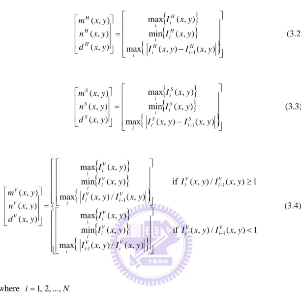
We build another background model with the minimum value ([nH( , ),x y nS( , ),x y nV( , )]x y ) and maximum value ([mH( , ),x y mS( , ),x y mV( , )]x y ) in

each HSV domain. Then, we also record the inter-frame ratio in the brightness information and the inter-frame different in the chromatic information. Similarly, we use the same background video to build another background model. Suppose the observed image frame sequence that contains N consecutive images. I_iH

( )

x y is the , pixel’s hue value at

( )

x,y of the i-th image frame. I_iS

( )

x y is the pixel’s saturation , value at

( )

x,y of the i-th image frame. I_iV

( )

x y is the pixel’s brightness value at ,

{

}

{

}

{

}

           − =           − ( , ) ) , ( max ) , ( min ) , ( max ) , ( ) , ( ) , ( 1 i y x I y x I y x I y x I y x d y x n y x m H i H i i H i i H i H H H (3.2)

{

}

{

}

{

}

           − =           − ( , ) ) , ( max ) , ( min ) , ( max ) , ( ) , ( ) , ( 1 i y x I y x I y x I y x I y x d y x n y x m S i S i i S i i S i S S S (3.3)

{

}

{

}

{

}

{

}

{

}

{

}

            <             ≥             =           − − − 1 ) , ( / ) , ( if ) , ( / ) , ( max ) , ( min ) , ( max 1 ) , ( / ) , ( f i ) , ( / ) , ( max ) , ( min ) , ( max ) , ( ) , ( ) , ( 1 1 -i 1 1 i y x I y x I y x I y x I y x I y x I y x I y x I y x I y x I y x I y x I y x d y x n y x m V i V i V i V i i V i i V i V i V i V i V i i V i i V i V V V (3.4) where i=1, 2,...,N

3.1.2 Foreground Object Extraction

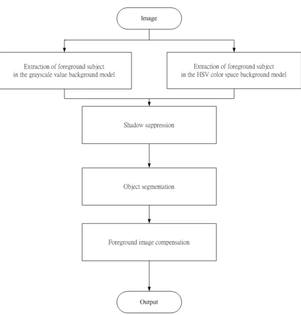
Fig. 3.1 shows the framework we apply to foreground subject extraction. Our framework of foreground subject extraction is composed of four components. The first component is foreground subject extraction in the grayscale value and the HSV color space background models. The second component is the shadow suppression.

classified to the background.

Fig. 3.1The framework we apply to foreground subject extraction.

Foreground objects can be segmented from every frame of the video stream. Each pixel of the video frame is classified to either a background or a foreground pixel by the difference between the background model and a captured image frame. First, we utilize the maximum grayscale value mgray

( )

x,y , minimum grayscale value n

( )

x,y

( )

model to segment a foreground by      − > + < = otherwise , 255 ) ) , ( ( ) , ( and ) ) , ( ( ) , ( if , 0 ) , ( 1 µ µ k y x n y x I k y x m y x I y x I _it gray gray t i foreground (3.5)

where I_it(x,y) is the intensity of a pixel which is located at

( )

x,y , I1foreground(x,y) is the gray level of a pixel in binary image, µ is the median of all dgray

( )

x,y , and k is a threshold. Threshold k is determined by experiments according to different environments. The value of k affects the amount of information retained in binary image I1foreground(x,y).

On the other hand, we utilize the maximum value V

(

,

)

m x y , minimum value

(

,

)

V

n x y and maximum inter-frame value ratio V

(

,

)

d x y of the HSV color space

background model to segment the foreground pixel by

     < < = otherwise , 255 ) , ( ) , ( / ) , ( or ) , ( ) , ( / ) , ( if , 0 ) , ( 2 y x d k y x n y x I y x d k y x m y x I y x I _iV V _V V V V V V i foreground (3.6)

where I_iV

(

x y is the intensity of a pixel which is located at ,

)

( )

x,y , I2foreground(x,y) is the gray level of a pixel in a binary image, k is a threshold, determined by light _V

sufficiency of the scene. k will be reduced for in-sufficient light condition and V

3.1.3 Shadow Suppression

The pixels of the moving shadows are easily detected as the foreground pixel in normal condition. Because the shadow pixels and the object pixels share the important visual feature: motion model. For this reason, the moving shadows cause object merging and object shape distortion. Therefore, we need to remove the shadow by using the shadow filter. We assume that the observed intensity of shadow pixels is directly proportional to incident light. Consequently, shadowed pixels are scaled versions (darker) of corresponding pixels in the background model [24].

In the first place, we build the shadow filter in the grayscale value. Let B(x,y)

be the background image formed by temporal median filtering, and I(x,y) be an image of the video sequence. For each pixel (x,y) belonging to the foreground, consider a 3×3 template T_xy such that T_xy(m,n)=I(x+m,y+n) , for

1 1

, 1

1≤ ≤ − ≤ ≤

− m n (i.e. T corresponds to a neighborhood of pixel _xy (x,y)). Then,

the NCC between template T and image B at pixel _xy (x,y) is given by:

) , ( ) , ( ) , ( xy T B x y E E y x ER y x NCC = (3.7) where

∑ ∑

∑ ∑

∑ ∑

− = =− − = =− − = =− = + + = + + = 1 1 1 1 2 1 1 1 1 2 1 1 1 1 ) , ( ) , ( ) , ( ) , ( ) , ( ) , ( n m xy T n m B n m xy n m T E n y m x B y x E n m T n y m x B y x ER xy (3.8)

If a pixel (x,y) is in a shadowed region, the NCC in a neighboring region T _xy

should be large, and the energy

xy

T

E of this region should be lower than the energy )

, (x y

E_B of the corresponding region in the background images. There, we get

    ≥ < = otherwise , foreground ) , ( and ) , ( shadow, ) , ( 1 NCC x y L E E x y y x S ncc Txy B (3.9)

where S1(x,y) is the binary image, and L_ncc is a fixed threshold. If L_ncc is low, several foreground pixels may be misclassified as shadow pixels. On the other hand, selecting a large value of Lncc, then the shadow pixels may not be detected.

We know that the shadow pixels have similar chromaticity but lower brightness than the background model. Therefore, we can detect the shadow in the HSV color space. We analyze the points which are possible moving object that are detected above. Building another shadow filter S2 for each ( , )x y point as follows:

       < − < − < − = otherwise , foreground ) , ( ) , ( ) , ( and ) , ( ) , ( ) , ( and 0 ) , ( ) , ( if shadow, ) , ( 2 y x d k y x m y x I y x d k y x m y x I y x n y x I y x S S S S S i H H H H i V V i (3.10)

where IiH( , )x y ,IiS( , )x y , and IiV

(

x y are respectively the HSV channel of a pixel ,

)

located at

( )

x,y , and S2(x,y) is one of the shadow filter to class the pixel in the moving shadow. Values kS and kH are selected threshold values that used to

We extract the foreground objects from the two background models. Setting a hard threshold for each background model, we obtain the foreground objects which have less noise, but missing some foreground objects. Therefore, using the union is better than the intersection. Because of using the union can increase the foreground with less noise. Finally, the foreground subject is defined as:

I_foreground(x,y)=S1(x,y)∨S2(x,y) (3.11)

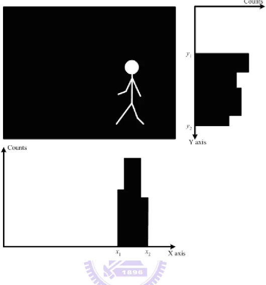
3.1.4 Object Segmentation

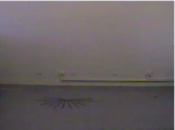
According to the binary image I_foreground segmented by above, we extract the region of foreground object as minimum as possible. Foreground region extraction can use a simply method by setting a threshold on the histograms in X-axis and Y-axis. Fig. 3.2 shows an example of foreground region extraction. We utilize the binary image that the binary image is projected on X-axis and Y-axis. The region we interest in that has higher counts in the histogram. We obtain the boundary coordinates x1, x2

of X-axis and y1, y2 of Y-axis from the projection histogram. We can use these

boundary coordinates as corners of a rectangle to extract foreground region.

3.1.5 Foreground Image Compensation

It is difficult to detect all the foreground pixels and remove all the shadows in the same time. When we want to remove shadow pixels, some foreground information

will be lost and that makes the foreground image be broken. In order to solve the problem, we will repair the foreground image by opening filter and closing filter.

After the four components, we extract the foreground objects. The rectangular image which contain foreground objects will be normalized to 128×96. Fig. 3.3 is the extracted foreground region.

Fig. 3.2The binary image is projected on X-axis and Y-axis.

3.2 Background Update

If we move indoor facilities, they will be detected as foreground pixels and the activity recognition will be misclassified. Therefore, we have to update background models in order to avoid above state occurring. Background models will be updated if the video does not vary for a long time and there is nobody in the scene. By Eq. (3.12), we calculate how many times the binary values are unchanged.

   + = = − otherwise ), , ( ) , ( ) , ( if , 1 ) , ( ) , ( 1 y x update y x I y x I y x update y x update t foreground t foreground (3.12)

where Itforeground(x,y) is the gray level of a pixel in binary image and it is located at

) ,

(x y . Value update(x,y) is a record of how many times It_foreground(x,y) remains unchanged.

By skin color detection, we can discriminate that there are someone or not. First, the input image is transfer to the normalized RGB color space by:

B G R R r + + = (3.13) B G R G g + + = (3.14)

According to Soriano and Martinkauppi [25], the boundary of skin tone in the r-g plane is defined as follow:

1452 . 0 0743 . 1 3767 . 1 ) (r =− r2 + r+ f_upper (3.15) 1766 . 0 5601 . 0 7760 . 0 ) (r =− r2 + r+ flower (3.16)

If a pixel satisfies the following four conditions, it will be labeled as skin pixel. Therefore, we know there is a person or not.

(3.17) ) ( nd ) (r a g f r f g > _lower < _upper (3.18) 0004 . 0 ) 33 . 0 ( ) 33 . 0 (r− 2 + g− 2 ≥ (3.19) B G R> > (3.20) 45 ≥ − G R

3.3 Down-sampling the Video Stream

Physical constraints on the architecture of human bodies’ induce rhythmic and repetitive patterns of motion limited within a certain frequency. Because cameras usually capture image frames in high frequency, i.e., 30 frames /sec. There is almost no difference between two consecutive image frames for a normal recording of 30 frames per second. Hence, we can down-sample the video frame instead of using all the 30 frames captured in a second. Down-sampling can also reduce the intensive computation and memory load. It is difficult to select the key posture as a result of different actions with different cycles.

The action cycle is defined as backing to repeat the same attitude time. In our daily life, some of the most universal and frequently performed actions are walking, jog and running. According to the statistics shown in KTH datasets, the mean of the walking cycle is 1.1s, jog cycle is 0.86s and running cycle is 0.67s. We observed running is short-period and walking is long-period. Fig. 3.4 is the walking video sequences. Fig. 3.5 is the jog video sequences, and Fig. 3.6 is the running video sequences.

Fig. 3.4 The walking video sequences.

Fig. 3.6 The running video sequences.

In our research, we compare using the same down-sampling rate with using the different down-sampling rate for different actions. Because of utilizing the 5:1 down-sampling rate for short-period actions, the key postures may be the same that cannot show the short-period action. Therefore, we will see whether down-sampling rate affects the human action recognition or not. The first method, we utilize 5:1 down-sampling rate for all actions to select the essential template image. The second method, we utilize 5:1 down-sampling rate for walking, 3:1 down-sampling rate for jog and 2:1 down-sampling rate for running to select the essential template image. Fig. 3.7 shows using 5:1 down-sampling rate to select the essential template images.

t₁ t₂ t₃ t₄ t₅ t₆ t template n₁ template n₂

Fig. 3.7 Using 5:1 down-sampling rate to select the essential template images.

These essential templates are transformed to a new space by eigenspace transformation (EST) and canonical space transformation (CST). The approximation will lose slight information of image with little differences, but it can decrease massive data dimensions. However, two similar image frames will converge to two

near points after eigenspace and canonical space transformation. The images of similar postures done by difference people also barely converge to one point. Consequently, we select only essential templates rather than use all sequences for human activity recognition.

Combining both EST and CST, each image frame is transformed to a (c–1)-dimensional vector [26]. Assume that there are n training models and c clusters in the system. Therefore, we have Nt templates, where Nt is equal to n multiplied by c.

Let gi,j be a vector of template image of the j-th training model and the i-th category

and ti,j be the transformed vector of gi,j. ti,j is computed by

n j c i j i j i, =H⋅g, , =1,2,, ; =1,2,, t (3.21)

where H denotes the transformation matrix which combine EST with CST and n is the total number of posture images in the i-th cluster. ti,j is a (c–1)-dimensional vector

and each dimension is supposed to be independent. Hence, ti,j is rewritten as

[

₁

]

T , 2 , 1 , , , , , − = c j i j i j i j i t t  t t (3.22)

The transformation of each training model’s templates is treated as a mean vector. That is,

∑

= = n j j i i n 1 , 1 t μ (3.23)

where i is the number of template categories.

The standard deviation vector of the m-th dimension is computed by

(

)

1 1 1 2 , − − =

∑∑

= = t c i n j m i m j i m N t µ σ (3.24) where m=1, 2, ,c−1.

3.4 Construction of Fuzzy Rules from Video Stream

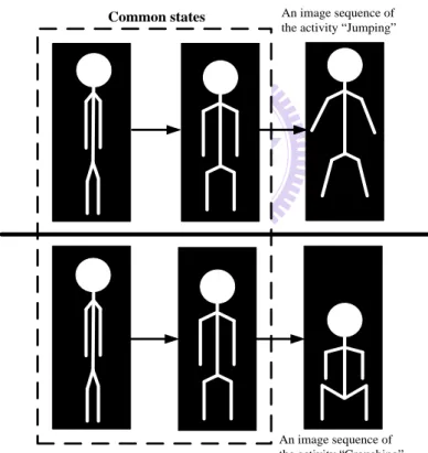
For human activity classification, temporal relationships of postures in video sequence are important information. Human’s actions may have similar postures in two different activity sequences. Therefore, only one image frame is utilized to classify the action that is prone to wrong. For example, the actions of “jumping” and “crouching” both have the same postures called common states as shown in Fig. 3.8. Besides, the posture sequence of each activity is dissimilar in different people.

An image sequence of the activity “Jumping”

An image sequence of the activity “Crouching”

Common states

Fig. 3.8 Common states of two different activities.

Hence, we propose a method which not only combines temporal sequence information for recognition but also is tolerant to variation of actions done by

We use the membership degree to represent the feature’s possibility of each cluster. We choose the Gaussian type membership function to represent the key posture’s features, because the Gaussian type membership function can reflect the similarity of the input feature vector to a key posture template vector.

Firstly, when the k-th training image frame xk is inputted, the feature vector ak is

extracted by

a_k =Hx_k. (3.25)

where H denotes the transformation matrix and ak can be rewritten as

a_k =

[

a_k1,a_k2,,a_kc−1

]

T. (3.26) If we assume that the dimensions of the feature vectors are independent, then we can compute the similarity between the training vector ak and each template vector.

Let Σ denote the covariance matrix of all essential template vectors and Ci denote the

i-th class of essential templates. The membership function is given by

∏

− = − −         − − =    _{− − −} = = 1 1 2 2 , 1 2 1 2 1 , ) ( 2 1 exp 2 1 ) ( ) ( 2 1 exp ) 2 ( 1 ) ( M c m m m j i m k m T c i k i a C r σ µ σ π π μ a Σ μ a Σ a k k k

(3.27)

where j is the training model number, ri,k denotes the grade of membership function

in category i of the k-th image frame and σm is the m-th dimensional variance of the

k i k r p _, i max arg = (3.28)

We obtain which category the image belongs to, but that is a single image. Recognizing the human action is using three consecutive posture sequences instead of a single posture. Therefore, we combine three consecutive posture sequences to a group (I1, I2, I3) and transfer the group to the feature vector (a1, a2, a3). Assume we

have c categories. There are c3 combinations of the feature vector. By Eq. (3.28), the feature vector (a1, a2, a3) is represented to (p1, p2, p3).

In [18], fuzzy rules are generated by learning from examples. The generated rules are the follow form:

“IF antecedent conditions hold, THEN consequent conditions hold.”

The number of antecedent conditions equals the number of features and the antecedent conditions are connected by “AND”. For example, an image sequence (Image 1, Image2, Image3) with its category is D1. We express that in vector format.

Eq. (3.29) is showing the vector format.

[

P1,P2,P3;D1

]

(3.29)

Suppose that Image 1, Image2 and Image 3 belong to category 1, category 2 and category 3 respectively. Therefore, the image sequence (Image 1, Image2, Image3) is transferred to (P1, P2, P3). Then, a rule is generated by the image sequence.

P1 P2 P3

Fig. 3.9 A fuzzy rule learned to classify action.

Rule 1. IF I is ₁ P AND ₁ I is ₂ P AND ₂ I is ₃ P₃ , THEN the activity is D1.

After the learning step of different actions, some conflicting rules may be generated. The conflicting rules have the same image sequence but different activity. Therefore, we have to choose one from a set of conflicting rules. To this end, we choose the rule that is supported by a maximum number of training examples. Furthermore, to prune redundant or inefficient fuzzy rules, if the number of examples supporting a rule is less than a threshold, the rule is excluded from the set of rules.

3.5 Classification Algorithm

To obtain the action for an input video stream, we utilize the background model to extract foreground objects from the image frames. Then, we use down-sampling rate to classify the three consecutive postures. These images will be obtained by the following procedures:

1. Foreground subject extraction 2. Normalization

3. Transformation by EST and CST

After these procedures and constructing the rule base, we can compute the similarity between current image sequences (Ik-2, Ik-1, Ik) and each rule in the rule

base by the membership function which is given by

∏

− = − −         − − =    _{− − −} = = 1 1 2 2 , 1 2 1 2 1 , ) ( 2 1 exp 2 1 ) ( ) ( 2 1 exp ) 2 ( 1 ) ( M c m m m j i m k m T c i k i s C s r σ µ σ π π μ s Σ μ s Σ k k k

(3.30)

where Σ denote the covariance matrix of all essential template vectors, Ci denote the

i-th class of essential templates and j is the training model number. σis the standard deviation of all essential templates. ri,k denotes the grade of membership function in

For example, given a rule, “IF Ik-2 is Pn1 AND Ik-1 is Pn2 AND Ik is Pn3, THEN

the action is Dn.” we compute the similarity degree of each image. We obtain the membership degrees (rk-2,n1, rk-1,n2, rk,n3) by Eq. (3.30). Then, we have to calculate the

firing strength (FS) of the rule. The sum is used to compute the firing strength that is defined as follows: 3 , 2 , 1 1 , 2n k n kn k r r r FS = ₋ + ₋ + (3.31)

Hence, we can compute the firing strength of each fuzzy rule which is in the rule base. Moreover, we will also investigate to the average value of maximal top-3, top-5, top-7, and top-9 firing strength of the rules with the same action to recognize the human action. Fig. 3.10 shows that take top-3 as an example, the similarity between three consecutive down-sampled images and each action that we average the maximal top-3 firing strength of the rules which have the same actions. After that, the action which has the highest average value of similarity is selected. Because of the major factors to separate the walking, jog and running is not templates but the velocity, therefore we include the velocity factor to recognize the human actions. We utilize the velocity to determine the actions and the fuzzy rules to determine the direction.

Chapter 4 Experimental Results

In our experiment, we tested our system on videos. We took the Weizmann databases, KTH databases and our LAB databases. We took our LAB databases at the 5th Engineering Building in NCTU campus. The light source is fluorescent lamp and stable. The background is not complex and we equip a table in the scene. The camera has a frame rate of thirty frames per second and image resolution is 320 240×

pixels.

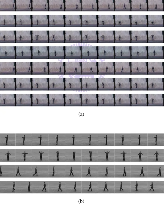
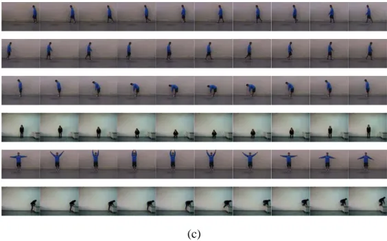
Fig. 4.1 and Fig. 4.2 show the environment of our LAB databases. In our LAB databases, the person performed several actions: “walking from left to right,” “walking from right to left,” “bend,” “crouch,” “climbing up,” and “waving.” The action “climbing up” is to climb up on the table from the ground. Fig. 4.3 shows the examples of actions from Weizmann databases, KTH databases and our LAB databases.

(a)

(c)

Fig. 4.3 Example video sequence used in our experiments. (a) Typical video sequences of Weizmann. From top to bottom: walk, bend, jack, jump, side, wave1 and wave2, respectively. (b) Typical video sequences of KTH. From top to bottom: boxing, wave, walking from left to right and walking from right to left, respectively. (c) Typical video sequences for actions of our LAB. From top to bottom: walking from right to left, walking from left to right, bend, crouch, wave and climbing up, respectively.

4.1 Background Model and Object Extraction

A background model is used for segmenting the foreground subject or object. In our system, we first record a video with no subject in environment to build the background models. If the grayscale value and the HSV color space background models are complete, we will extract the foreground pixels by using Eq. (3.5) and Eq. (3.6) in Section 3.1.2.

In order to get the optimal result of object extraction, we have to adjust the threshold in our system. In the grayscale value and the HSV color space background models, we set k =2.3 in Eq. (3.5) and kv =1.4 in Eq. (3.6) to extract foreground pixels. Fig 4.4 shows an example of foreground extraction. Fig. 4.4(a) is a frame which obtained from background video. Fig. 4.4(b) is an image frame of the video stream. Fig. 4.4(c) is the result of the image frame transferred to grayscale value. Fig. 4.4(d) is the binary image after using shadow filter, closing filter and opening filter. Fig. 4.4(e) is the extracted foreground region.

(a) (b)

(c) (d)

(e)

Fig 4.4 Showing an example of foreground extraction. (a) Background image. (b) Input image. (c) Grayscale value image. (d) Binary image. (e) Extraction foreground image.

4.2 Fuzzy Rule Construction for Action Recognition

We construct the template model and the fuzzy rule database with the training data. We first utilize 5:1 down-sampling rate for walking, jog and running to select the essential templates. On the other hand, we utilize 5:1 down-sampling rate for walking, 3:1 down-sampling rate for jog and 2:1 down-sampling rate for running to select the essential templates. Thus, compare using the same down-sampling rate with using the different down-sampling rate, and we will know whether down-sampling rate affects the human action recognition. Fig. 4.5 is an example of some templates that using the same down-sampling rate. Fig. 4.6 shows using the different down-sampling rate to select the essential templates.

Fig. 4.5 Some essential templates use the same down-sampling rate. From top to bottom: walking, jog and running, respectively.

Fig. 4.6 Some essential templates use the different down-sampling rate. From top to bottom: walking, jog and running, respectively.

Furthermore, we chose five kinds of essential templates for “walking from right to left,” “walking from left to right,” “bend,” “crouch,” “climbing up,” “waving,” “boxing,” “jack,” respectively; four for “side,” “wave1,” “wave2” and three for “jump.” There are totally 30 kinds of essential templates in Weizmann databases, 20 kinds of essential templates in KTH databases and 30 kinds of essential templates in our LAB databases. Each essential template is a cluster with four similar key postures which are selected from four different training persons. Fig 4.7, Fig. 4.8, and Fig. 4.9 are the examples of essential templates of respective datasets.

Class 1 Class 3 Class 7

Class 9 Class 11 Class 14

Class 17 Class 19 Class 21

Class 24 Class 27 Class 29

Class 1 Class 3 Class 7

Class 8 Class 9 Class 10

Class 11 Class 12 Class 14

Class 16 Class 18 Class 19

Class 1 Class 3 Class 6

Class 9 Class 12 Class 14

Class 17 Class 19 Class 23

Class 25 Class 26 Class 29

After determining the standard deviation vectors, the corresponding training video frames are inputted. The relationship between each image frame and each template is calculated by using Eq. (3.27) in Section 3.4. We gathered three consecutive down-sampled images as a group in order to include temporal information. The interval between each of these three images is determined by the down-sampling rate which is the same as in template selection phase and learning phase. Therefore, we gathered three images from different start points to train fuzzy rules. Taking 5:1 down-sampling rate for examples: the first frame, the 6-th frame and the 11-th frame are gathered together as an input training data; the second frame, the 7-th frame and the 12-th frame are gathered together as another input training data; the third frame, the 8-th frame and the 13-th frame are gathered together as another input training data, etc. Different start points of image frames are used for training fuzzy rules in our experiment, because the starting posture of testing video may not be the same. By utilizing different start points, the system is able to learn and then classify the actions at any time instant.

The group of the three images is converted to the posture sequence which has the maximum summation of three membership function values in Eq. (3.27). Each posture sequence will the consequent action of the rule with maximal value. If the corresponding rule is not existent, a new rule is built in the form of IF-THEN which is represented in Section 3.4.

Table I

Some of the Obtained Fuzzy Rule Base

Number Image 1 Image 2 Image 3 Class

1 P1 P1 P1 WRL 2 P1 P1 P2 WRL 3 P1 P1 P3 WRL      30 P4 P11 P12 WLR      60 P3 P13 P14 Bend      80 P13 P16 P17 CROUCH      91 P2 P18 P18 WAVE      129 P27 P28 P10 CUP 130 P28 P7 P7 CUP 131 P28 P28 P10 CUP

4.3 The Recognition Rate of Activities

In order to calculate the recognition rate of activities, we use videos to test the human action recognition system. Each of video includes several actions in our experiment. Then, we input the testing video from different starting frames which is similar to the way for the training fuzzy rules. Namely, we recognize the video from the first frame, the second frame, the third frame and the fourth frame, etc. with the sampling intervals of five frames. Hence, there are many video databases for testing. The WRL is the activity “walking from right to left,” WLR is the activity “walking from

“running from left to right,” and CUP is the activity “climbing up.” The frame based

accuracy is the total number of correct recognition divide by the total number of recognitions done. The following tables show the accuracy by using the video bases. Fig. 4.10 shows the statistic velocity of walking, jog and running from the KTH dataset and we normalize the statistic result. Fig. 4.11 shows the regularization result.