Adaptive radio maps for pattern-matching localization via inter-beacon co-calibration

(1)

Contents lists available atSciVerse ScienceDirect

Pervasive and Mobile Computing

journal homepage:www.elsevier.com/locate/pmc

Adaptive radio maps for pattern-matching localization via inter-beacon

co-calibration

Chi-Chung Lo

∗

, Lan-Yin Hsu, Yu-Chee Tseng

Department of Computer Science, National Chiao-Tung University, Hsin-Chu, 30010, Taiwan

a r t i c l e i n f o

Article history:

Received 24 February 2011

Received in revised form 30 December 2011 Accepted 2 January 2012

Available online 11 January 2012 Keywords:

Localization Location-based service Trajectory tracking Wireless sensor network

a b s t r a c t

A growing number of location-based applications are based on indoor positioning, and much of the research effort in this field has focused on the pattern-matching approach. This approach relies on comparing a pre-trained database (or radio map) with the received

signal strength (RSS) of a mobile device. However, such methods are highly sensitive to

environmental dynamics. A number of solutions based on added anchor points have been proposed to overcome this problem. This paper proposes an approach using existing beacons to measure the RSS from other beacons as a reference, which we call inter-beacon

measurement, for the calibration of radio maps on the fly. This approach is feasible because

most current beacons (such as Wi-Fi and ZigBee stations) have both transmitting and receiving capabilities. This approach would relieve the need for additional anchor points that deal with environmental dynamics. Simulation and experimental results are presented to verify our claims.

1. Introduction

Location-based services (LBS) are highly popular applications in mobile and wireless technology [1], and location tracking is the core problem [2–4]. GPS is currently the most widely used technology for location tracking in outdoor environments; however, due to effects such as shadowing, GPS cannot be used indoors.

Recently, considerable research has been dedicated to the development of wireless networks as an infrastructure for indoor location tracking. One promising approach is the pattern-matching technique [5–8], which is capable of meter-level accuracy. It uses the received signal strength (RSS) of the radio frequency emitted by the stations of wireless networks as reference. We call these stations beacons. A pattern-matching system usually works in two phases: training and positioning. In the training phase, the operator collects the RSS of beacons at various training locations to form a database referred to as a the radio map. During the positioning phase, the mobile device compares its current RSS against the radio map to determine its location.

Fluctuations resulting from environmental dynamics are the major drawback of the pattern-matching approach. Temperature, humidity, and moving objects are all capable of disrupting the observed RSS, leading to deviations in the trained radio map. LANDMARC [9] is a solution relying on active RFIDs and training data obtained from online sources to perform indoor localization. LEMT [10] is another approach using anchor points to derive adaptive temporal radio maps to overcome this problem. However, all of these existing solutions rely on additional hardware to deal with environmental dynamics and to calibrate the radio maps.

This paper proposes a novel approach that allows for the self-calibration of radio maps without the need for additional hardware. Most current beacons (such as Wi-Fi APs and ZigBee nodes) have both transmitting and receiving capabilities.

∗_{Corresponding author.}

(2)

Using these beacons to observe the RSS from other beacons, which we call inter-beacon measurement, would enable the capture of current environmental dynamics and the calibration of radio maps on the fly.

The remainder of this paper is organized as follows. In Section2, we review some related works. In Section3, we propose a framework to enable inter-beacon measurement as well as two schemes to calibrate radio maps, based on data clustering and data regression. In Section4, we verify our results via simulations and practical experiments. Conclusions are drawn in Section5.

2. Background and related works

The implementation of radio-based wireless networks for indoor localization relies on either a radio-propagation model [11] or an empirical-fit model [12]. In a radio-propagation model, a multi-lateration mechanism is required to calculate the location of a device. The path loss of beacon b at a distance d is normally modeled as follows [13]:

Pr

(

d

,

b

) =

Pt

(

b

) −

PL

(

d0

,

b

) −

10

η

log10



d d0



+

N

(

0

, σ ),

(1)

where Pt

(

b

)

is the transmitting power of b, PL

(

d0

,

b

)

is the path loss at distance d0

, η

is an environment- and

hardware-dependent constant, d0 is a reference distance, and N

(

0

, σ)

is a zero-mean normal-distribution random variable.

Unfortunately, this model is not adequate for indoor environments with dynamically changing

η

and

σ

.

This study focuses on the empirical-fit model [5,14,15], also known as pattern-matching localization. Given a set of beaconsB

= {

b1

,

b2

, . . . ,

bm

}

and a set of training locationsL

= {

ℓ

1

, ℓ

2

, . . . , ℓn

}

in a sensing field, this method proceeds

through two phases. In the training phase, we measure the RSS vectors of all beacons at each training location

ℓi

over a period of time and create a feature vector

υi

= [

υi

_,₁

, υi

_,₂

, . . . , υi

_,_m

]

for

ℓi

, where

υi

_,j

∈

R is the average RSS from bj, j

=

1

. . .

m. These feature vectors are collected in a setV

= {

υ

₁

, υ

₂

, . . . , υn

}

, called the radio map. In the positioning phase, a mobile device measures its current RSS vector s

= [

s1

,

s2

, . . . ,

sm

]

and compares s againstV. The best matched one or ones in

Vare used to predict the current location of the device. In practice, we could also choose the nearest neighbor [5] and use probabilistic techniques [15] as a matching method. In [5], the nearest neighbor algorithm is applied to search for the best match according to Euclidean distances in the signal space. In [6], a probabilistic framework for localization is presented to handle fluctuations in signal strength. Generally, the probabilistic approach can more accurately reflect the dynamics associated with changes in RSS. Below, we review existing works from three perspectives: (1) techniques to improve scalability, (2) techniques to exploit history tracking information, and (3) techniques to handle RSS dynamics.

To improve scalability, it should be noted that all pattern-matching solutions rely on a large amount of training data. To deal with this issue, Refs. [16,17] propose clustering-based methods to reduce comparison costs. The main idea is to apply clustering techniques to divide a radio map into smaller sub-maps.

To exploit history tracking information, many researchers have used a sequence of positioning results to improve accuracy. In [18], Bayesian filters were developed to integrate multiple sources of sensing data. The key features of these filters are observation, prediction, and history models to remove unreliable data. For example, a tracking system is capable of exploiting the mobility history of users to speculate as to their trajectory [19]. By contrast, particle filters are used in [18] to reflect the probability densities of our beliefs based on previous measurements. In [20], the belief about a dynamic system at time t is represented as a probability distribution over the state space.

To deal with environmental dynamics, [9] used RFID tags as references for RSS distribution to aid in localization. In [21], stationary emitters and sniffers were used to determine the training data and assist in indoor localization online. A sensor-assisted scheme was proposed in [22] to measure the current radio map. LEMT [10] is the first research to use anchor points to derive adaptive temporal radio maps capable of overcoming environmental dynamics. However, these approaches all required additional hardware to deal with environmental dynamics and to calibrate the radio maps.

3. Adaptive radio maps via inter-beacon measurement

An inherent limitation of the pattern-matching localization method is the problem of signal instability. To deal with this issue, we propose a method based on inter-beacon measurement. We have observed that most beacons in use have both transmitting and receiving capabilities. Recruiting these beacons to measure the RSS of neighboring beacons, would enable the adaptive calibration of radio maps. Consider the example inFig. 1. Suppose that biand bjare two beacons and

ℓ

is a training location. In the training phase, let Siand Sjbe the RSSs of biand bjmeasured at

ℓ

, respectively. During the positioning phase, suppose that a device at

ℓ

measures the RSSs of biand bjas Si′and S

′ j, respectively. If

{

S ′ i

,

S ′ j

}

were to deviate too far from

{

Si,Sj

}

, it would be exceedingly difficult to determine whether the device is at position

ℓ

.

The concept behind the proposed inter-beacon measurement method is to add two tags, Si,jand Sj,i, during the training phase to represent the RSS of bias observed by bjand the RSS of bjas observed by bi. It the positioning phase, in addition to measuring S′

iand S ′

j, we also collect S ′

i,j(the RSS of bias observed by bj) and S′j,i(the RSS of bjas observed by bi). It is expected that using the set

{

Si,Sj,Si,j,Sj,i

}

collected in the training phase and the set

{

Si′

,

S

′ j,S′

i,j,S ′

j,i

}

collected in the positioning phase, would provide additional clues to determine whether the mobile device is located near

ℓ

.

(3)

Fig. 1. An example of inter-beacon measurement.

Fig. 2. Flow chart of the proposed solutions.

In the following, we formally define the problem as follows. We define a set of beaconsB

= {

b1

,

b2

, . . . ,

bm

}

and a set of training locationsL

= {

ℓ

₁

, ℓ

₂

, . . . , ℓn

}

in a sensing field. In the training phase, suppose that we measure the RSS vectors at each location

ℓi

to create the radio mapVin conjunction with the measurements among the beacons. The question is: In the positioning phase, how do we provide an adaptive radio mapV′_{, based on the current observations of inter-beacon}

measurement to facilitate the task of localization?

We propose two solutions as follows. The first solution uses information related to the inter-beacon measurement to cluster training data into multiple radio maps. To position a device, we first use the current inter-beacon measurement to select an appropriate radio map, from which we choose the closest location. This solution is based on the assumption that there should be a high correlation between each inter-beacon measurement and its corresponding training cluster. Therefore, the current inter-beacon measurement is a good indicator of the cluster to be used during the positioning phase. Conversely, the second solution involves the use of inter-beacon measurements to interpolate the current radio map. This solution is based on the assumption that the correlation between each inter-beacon measurement and its corresponding training data can be predicted using a linear regression model. Both solutions comprise three phases, as illustrated inFig. 2.

3.1. Solution 1: Clustering-based scheme

Beacon-assisted training phase: In each training location, we collect two types of RSS: beacon-to-device RSS (BD-RSS) and beacon-to-beacon RSS (BB-RSS). BB-RSSs reflect the environmental characteristics when the corresponding BD-RSSs are collected. Specifically, multiple (BD-RSS, BB-RSS) pairs will be collected at each

ℓi

. Each BD-RSS is a vector with the format

υ

(x)

i

= [

υ

(x)

i,j

]

j=1...m, where x is the timestamp of when the vector was measured and

υ

( x)

i,j is the RSS of beacon bjmeasured at

ℓi

. When

υ

_i(x)is recorded, the system also records the RSS of bjmeasured by bk, denoted by

µ

(i,xj),k. These measurements

(4)

are recorded in a BB-RSS vector

µ

(_ix)

= [

µ

(_i_,x_j)_,_k

]

_j=1...m,k=1...m,j̸=k. In practice, it is difficult to ensure that a BD-RSS and a BB-RSS are taken at precisely the same time, considering that beacons have regular jobs to perform. A degree of timing difference is acceptable as long as the environment remains roughly similar between measurements. For simplicity, we still use the same superscript (x) here. The combination (

υ

_i(x)

, µ

(_ix)) is called a (BD-RSS, BB-RSS) pair measured at time x for

ℓi

. The collections are maintained in a training databaseT

= {

(υ

_i(x)

, µ

_i(x)

) | ∀ℓi

∈

L

, ∀

x

}

.

To enable inter-beacon measurement, each beacon must switch to receive mode from time to time. This can be performed easily by modern Wi-Fi and ZigBee interfaces. In addition, to increase the diversity of databaseT, the measuring time xs should be as diversified as much as possible. For example, we could conduct measurements on sunny and rainy days, on working days and holidays.

Data clustering phase: Because databaseT is collected with diversity in mind, we suggest partitioningT into several subsets, each called a radio map, according to their similarity. Below, we propose a modified k-means clustering algorithm [7,

23] to achieve this goal.

1. Apply the k-means algorithm to partitionT into k subsets using the BB-RSS of each (BD-RSS, BB-RSS) pair as the key. The k-means process involves multiple data-clustering iterations in which these keys are compared. Specifically, when comparing the similarity between two (BD-RSS, BB-RSS) pairs P

=

(υ

_p(x)

, µ

(_px)

)

and Q

=

(υ

_q(y)

, µ

(_qy)

)

, we define their distance as d

(

P

,

Q

) =





∀j,∀k

µ

(x) p,j,k

−

µ

(y) q,j,k



2

.

(2)

Here, a larger distance means a lower degree of similarity. Each iteration of the process generates k subsets. Intuitively, pairs with similar BB-RSSs (i.e., those measured under similar conditions) are inserted into the same subset.

2. Let the k subsets obtained in step 1 beT1,T2

, . . . ,

Tk. For eachTi, i

=

1

. . .

k, we define a feature vector forTibased on the BB-RSSs of the members ofTi. Specifically,Ti’s feature vector is

ωi

= [

ωj

,k

]

j=1...m,k=1...m,j̸=k, where

ωj

,k

=



(υ(x) p ,µ( x) p )∈Ti

µ

(x) p,j,k

|

Ti

|

.

(3) 3. The above definedTi,i

=

1

. . .

k, is not necessarily well-formed because a number of the training locations may not appear inTi(the k-means algorithm does not guarantee this property). To ensure thatTiis a well-formed radio map, we must check whether there exists at least one

(υ

p(x)

, µ

(px)

) ∈

Tifor each

ℓp

∈

L. If not, we compare the

ωi

ofTiagainst all (BD-RSS, BB-RSS) pairs for

ℓp

inT. The pair for which BB-RSS is most similar to

ωi

is added toTi. With this amendment,

Tibecomes well-formed.

In practice, for a given total number of t training samples, we set k

=

√

t. In addition, it should be noted that it is possible that multiple units of training data sampled at different times in the same training location may be inserted into the same radio map. This is because they may have similar environmental characteristics. These data may be averaged into a single unit or remain unchanged, depending on the localization algorithm used in the positioning phase.

Clustering-based positioning phase: When a device is required to determine its location, it measures its current BD-RSS vector, denoted by

υc

˜

= [ ˜

υc

_,_j

]

_j=1...m. It then submits

υc

˜

to the location server, which takes the following actions.

1. The location server first requests that all beacons measure the RSS of the others. The collected current BB-RSS vector is denoted by

µ = [ ˜µj

˜

_,_k

]

_j=1...m,k=1...m,j̸=k.

2. The location server then compares

µ

˜

against the

ωi

of eachTi. The distance between

µ

˜

and

ωi

is defined as

d

( ˜µ, ωi) =





∀j,∀k

 ˜

_µj

_,_k

−

ωj

_,_k



2

.

(4)

LetTibe the one for which d

( ˜µ, ωi)

is the smallest. We then selectTias the current radio map and compare

υc

˜

against the BD-RSS of each (BD-RSS, BB-RSS) pair inTi. When comparing the similarity of

υc

˜

and a BD-RSS

υp

, we define their distance as d

( ˜υc, υp) =





∀j

 ˜

_υc

_,_j

−

υp

_,_j



2

.

(5)

The location for which the corresponding BD-RSS is most similar to

υc

˜

is estimated as the location of the device. In Step 2, a BB-RSS must be measured in response to every location query. To reduce overheads, the location server can periodically collect BB-RSS vectors, such that the most recent is regarded as

µ

˜

.

(5)

0 10 20 30 40 50 Y axis 0 10 20 X axis 30 40 50 Walls Path1 Path2 Path3

Fig. 3. The simulated environment. 3.2. Solution 2: Regression-based scheme

The Beacon-assisted training phase is the same; therefore, we will only discuss the following two phases.

Data regression phase: Recall that for each training location

ℓp

, we have already collected a number of (BD-RSS, BB-RSS) pairs inT. Given the current BB-RSS, we can use these pairs to predict the current BD-RSS vector at

ℓp

using a regression method. LetTpbe the set of (BD-RSS, BB-RSS) pairs collected at

ℓp

. We assume the following linear relation:

υ

(x) p,i

=



∀x,∀j,j̸=i

aj

×

µ

(px,)i,j

+

b

.

(6)

Intuitively, we use terms on the right-hand side to predict the RSS of bimeasured at

ℓp

. Eq.(6)can be established for each pair inTp, resulting in







µ

(1) p,i,1

· · ·

µ

(1) p,i,m 1

...

· · ·

...

µ

(x) p,i,1

· · ·

µ

(x) p,i,m 1













Ap,i

×







a1

...

am b







  

Bp,i

=







υ

(1) p,i

...

υ

(x) p,i













Cp,i

.

(7)

Using least-squares analysis, we obtain

Bp,i

=

(

ATp,iAp,i)−1ATp,iCp,i

.

(8)

Note that if we continue increasing the number of training vectors, Bp,iwill also be changed. In practice, we can update

Bp,iperiodically to balance the computing cost and positioning accuracy. In addition, the size ofTpshould be bounded to ensure that computing Eq.(8)remains feasible.

Regression-based positioning phase: When a device must determine its location, it measures its current BD-RSS vector

υc

˜

and submits

υc

˜

to the location server, which then takes the following actions.

1. It first request all beacons measure the RSS of the others. Let the RSS of bimeasured by bjbe

µi

˜

,j.

2. Using the previously obtained Bp,i, the server then predicts the current RSS vector at location

ℓp

as

υp

˜

=

[ ˜

υp

_,₁

, ˜υp

_,₂

, . . . , ˜υp

_,_m

]

, where

υp

˜

_,_i

= [ ˜

µi

_,₁

, ˜µi

_,₂

, . . . , ˜µi

_,m,1

] ×

Bp,i

,

i

=

1

. . .

m.

3. We then compare

υc

˜

against each

υp

˜

for all training locations. The

ℓp

which provides the smallest distance d

( ˜υc, ˜υp)

is estimated as the location of the devices.

4. Simulation and experimental results

4.1. Simulation results

To verify our results, we simulated a 50 m

×

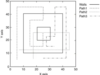
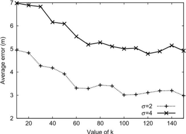
50 m sensing field with 12 beacons. Each beacon had a radio power of 15 dBm to ensure that the beacons could reach each other. Training locations were grid points separated by 1 m, and five samples were taken from each training location. To complicate the environment, a number of vertical and horizontal walls were placed on the field, as shown inFig. 3. Several roaming paths of users were simulated. Note that users may occasionally

(6)

Fig. 4. Impact of k in the clustering-based scheme.

pass walls; the purpose is to see how the scheme performs when there are sudden signal changes. We adopted the path loss model of RIM [24] and rewrote Eq.(1)as follows:

Pr

(

d

,

b

) =

Pt

(

b

) −

PLDOI

(

d

,

b

) −

PLWAF

(

d

,

b

) +

N

(

0

, σ).

(9)

In RIM, DOI stands for ‘‘degree of irregularity’’, and is used to control the amount of path loss in different directions, PLDOI

(

d

,

b

) =



PL

(

d0

,

b

) +

10

η

log10



d d0



×

Ki, (10)

where Kiis used to model the level of irregularity at degree i

(

i

=

0

..

359

)

,

Ki

=



1 if i

=

0

Ki−1

±

W

(

0

, β, φ) ×

DOI if i

=

1

..

359 (11)

where

|

K0

−

K359

| ≤

DOI and W

(

0

, β, φ)

is a zero-mean Weibull random variable with a slope parameter

β

and a scale

parameter

φ

. Here, we let

β =

1 and

φ =

0

.

1. The resulting PLDOI

₍

_d

_,

_b

₎

_{has non-isotropic and continuous properties. To} model the impact of indoor partitions and walls in such an environment, we employed a wall attenuation factor

(

WAF

)

[5],

PLWAF

(

d

,

b

) =

min

(

Nobs

,

Nmax

) ×

WAF

,

(12)

where Nobsis the number of walls crossed by a line-of-sight path, Nmaxis the maximum number of walls that can influence

PLWAF

₍

_d

_,

_b

₎

_{, and WAF is the amount of signal attenuation caused by a single wall. Note that P}

r

(

d

,

b

)

is a random variable, which may change at any moment.

The total simulation time was 1000 s. The moving speed of the users was set to 1 m/s and RSSs were measured every second. The default simulation parameters were Pt

(

b

) =

15 dBm, d0

=

1 m

, σ =

2 or 4, PL

(

d0

,

b

) =

37

.

3 dBm,

η =

3

.

3

,

DOI

=

0

.

01, WAF

=

3, and Nmax

=

4. We compared our scheme against the NNSS (nearest neighbor in signal space)

scheme [5]. We also simulated an ideal NNSS scheme, which assumes that the

η

used in the training phase is known in the positioning phase. For each measurement (including training and positioning phases), we randomly selected

η

in

[

3

.

1

,

3

.

5

]

and

[

2

,

4

]

to reflect the environmental dynamics. Below, we discuss our simulation results from four perspectives.

(1) The impact of k in the clustering-based scheme:Fig. 4shows the impact of k on positioning accuracy in the Clustering-based scheme when

σ =

2 and 4. In our simulation, 13

,

005 training samples were divided into k clusters. According to our simulation result, the Clustering-based scheme can continuously improve the average positioning errors for k

≤

60. However, for k

>

60, the average positioning error almost remains the same. In our experience, for given a total number of t training samples, setting k

=

√

t is a fairly good choice (in the above case k+110). We will adopt this setting in subsequent discussions.

(2) Comparison of positioning errors:Table 1shows the average positioning error of our scheme, as opposed to the NNSS and the ideal NNSS schemes under various combinations of

σ

and

η

values. Note that

σ

reflects the impact of environmental noise to those schemes, while

η

reflects the impact of temperature, humidity and various kinds of hardware-dependent dynamics. Compared to the NNSS scheme, the Clustering-based scheme reduces the average positioning error by 16%–28% and the Regression-based scheme reduces the average error by 35%–45%. In our experience, the Regression-based scheme performs slightly better than the Clustering-based scheme. For

σ =

2 and 4,Fig. 5(a) and (b) show the respective CDFs of the positioning errors of these schemes when

η

is in interval

[

3

.

1

,

3

.

5

]

. The ideal NNSS has maximum error distances of 4.5 m and 9.4 m, whereas the NNSS has maximum error distances of 14.8 m and 24.1 m, when

σ =

2 and 4, respectively. Under the same environment, the maximum error distances of the Regression-based scheme and the Clustering-based scheme are approximately 7.4–11.3 m and 8.4–13.2 m, respectively. All schemes suffer from increased noise levels. For

σ =

2 and 4,

(7)

Table 1

Average positioning errors in meters.

σ =2 σ =4 σ =2 σ =4 ηin [3.1, 3.5] ηin [3.1, 3.5] ηin [2, 4] ηin [2, 4] Ideal NNSS 1.446 2.991 1.522 3.201 Regression-based 2.398 4.101 2.655 4.188 Clustering-based 3.031 4.552 4.130 5.037 NNSS 3.692 6.401 4.757 7.144

Fig. 5. Comparisons of CDFs of positioning errors when (a)σ =2 andη ∈ [3.1,3.5], (b)σ =4 andη ∈ [3.1,3.5], (c)σ =2 andη ∈ [2,4], (d)σ =4 and

η ∈ [2,4].

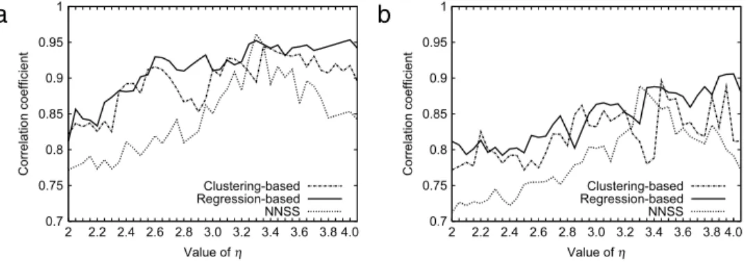
Fig. 6. Correlation coefficient of the used radio map and the current radio map versusηwhen (a)σ =2 and (b)σ =4.

Fig. 5(c) and (d) show the respective CDFs of positioning errors using these schemes when

η

is in

[

2

,

4

]

. A larger interval for the environment- and hardware-dependent constant

η

makes the resulting radio map more dynamic, thereby increasing the difficulty and errors associated with of our positioning.

(3) Correlation of radio maps: To explain why the Regression-based scheme performs slightly better than the Clustering-based scheme, we analyzed the correlation between the selected radio map and the current radio map. Theoretically, if we select a radio map with a high degree of correlation (i.e., similarity) with the current radio map, the pattern-matching approach should provide a positioning result with a high degree of accuracy. This is the main idea in [9,10,21,22] and in the proposed scheme. InFig. 6(a) and (b), we compare the correlation coefficients of the selected radio map with the current radio map when

σ =

2 and

σ =

4, respectively. Here, the correlation of two radio maps is defined as follows. Let

(8)

Fig. 7. Impact of beacon density on positioning accuracy. Table 2

Comparison of average and maximal positioning errors (in meters).

Regression-based Clustering-based NNSS

Average error 4.96 6.37 8.13

Maximum error 15.95 16.51 22.17

˜

υi

= [ ˜

υi

_,_j

]

_j=1...mbe the RSS vector in the selected radio map and

υi

= [

υi

,j

]

j=1...mbe the RSS vector in the current radio map. Also, let X be the set of

[ ˜

υi

_,_j

]

_i=1...n,j=1...mand Y be the set of

[

υi

,j

]

i=1...n,j=1...m. Then, the correlation coefficient

ρX

,Y of two radio maps can be derived as

ρX

,Y

=

cov

(

X

,

Y

)

σX

σY

,

(13)

where cov

(

X

,

Y

)

is the covariance between X and Y ,

σX

is the standard deviation of X , and

σY

is the standard deviation of Y . Here, we set

η =

2–4 in the positioning phase to generate the current radio map and compare it against the radio maps picked by the NNSS, the Regression-based scheme, and the Clustering-based scheme (

η

of the radio map picked by the NNSS is 3.3). According to our simulation results, the Regression-based scheme has a better correlation than the current radio map, which explains its better performance.

(4) The impact of the density of beacons:Fig. 7shows the impact of using various numbers of beacons. Although twelve beacons were used in the field, we randomly selected a few to measure the signal strengths from nearby beacons. (The other beacons were prohibited from conducting inter-beacon measurements.) For the NNSS and the ideal NNSS schemes, such a change did not impact performance. For the proposed scheme, using additional beacons with inter-beacon measurement capability improved the capture of environmental dynamics and thus improved positioning accuracy. These trends are illustrated inFig. 7.

4.2. Experimental results

We further verified our results in a real environment, as shown inFig. 8. Note that the environment has a dense deployment of WiFi access points (normally more than 20–40). Training data were collected from 124 training locations, each separated by 2 m, in a public corridor. In each training location, we randomly collected 100 samples between July 1, 2010 and October 30, 2010. Each sample comprised an average of ten base stations. In total, thirty five base stations were observed. We also collected data at 117 testing locations, each separated by 1 m, for testing purposes. In the experiment, the goal was to verify the existence of signal fluctuations and the capability of the proposed scheme to handle such environmental dynamics. Note that unlike the earlier simulations, we were unable to control the values of

η

and

σ

. Therefore, we were unable to compare the ideal NNSS scheme with the proposed scheme.

We randomly selected two training locations and observed the measurements.Fig. 9(a) and (b) show the measured RSS distributions from beacons in two locations. Clearly, the signal fluctuation problem does exist in real situations.

Based on the above setting, we conducted a number of localization experiments.Table 2shows the average positioning error and the maximum positioning error of the proposed scheme, compared with the NNSS. Compared toTable 1, all schemes returned higher positioning error in the real experiment. However, the Clustering-based scheme reduced the average error by 22%, and the Regression-based scheme reduced the average error by 43%. These results verify the effectiveness of the proposed approach.

(9)

Fig. 8. Experiment environment at the Computer Science Building, National Chiao Tung University. Training locations are labeled by dots (•). Testing data were collected along the dotted line between A and B.

Fig. 9. Measured RSS distributions from beacons in two locations. 5. Conclusions

In conclusion, we have proposed a novel indoor localization model in which beacons measure the signal strengths of other beacons. Thus, beacons not only serve as localization tools, but also serve as calibration tools to self-adjust the radio maps on-the-fly. We proposed two schemes to calibrate the radio map. The first scheme is based on data clustering, which we call the Clustering-based scheme, and the second scheme is based on data regression, which we call the Regression-based scheme. According to our results, both schemes are capable of improving localization accuracy with the Regression-based scheme performing slightly better than the Clustering-based scheme.

References

[1] S.J. Vaughan-Nichols, Will mobile computing’s future be location, location, location? Computer 42 (2) (2009) 14–17.

[2] I. Constandache, R. Choudhury, I. Rhee, Towards mobile phone localization without war-driving, in: Proc. of IEEE INFOCOM, 2010.

[3] C.-C. Lo, C.-P. Chiu, Y.-C. Tseng, S.-A. Chang, L.-C. Kuo, A walking velocity update technique for pedestrian dead-reckoning applications, in: Proc. of IEEE Int’l Symposium on Personal Indoor and Mobile Radio Communications, PIMRC, 2011.

[4] A. Kushki, K.N. Plataniotis, A.N. Venetsanopoulos, Intelligent dynamic radio tracking in indoor wireless local area networks, IEEE Trans. Mob. Comput. 9 (3) (2010) 405–419.

[5] P. Bahl, V.N. Padmanabhan, RADAR: an in-building RF-based user location and tracking system, in: Proc. of IEEE INFOCOM, 2000.

[6] T. Roos, P. Myllymäki, H. Tirri, P. Misikangas, J. Sievänen, A probabilistic approach to WLAN user location estimation, Int. J. Wirel. Inf. Netw. 9 (3) (2002) 155–164.

[7] S.-P. Kuo, B.-J. Wu, W.-C. Peng, Y.-C. Tseng, Cluster-enhanced techniques for pattern-matching localization systems, in: Proc. of IEEE Int’l Conference on Mobile Ad-Hoc and Sensor Systems, MASS, 2007.

[8] J. Letchner, D. Fox, A. LaMarca, Large-scale localization from wireless signal strength, in: Proc. of the Nat’l Conference on Artificial Intelligence, AAAI, 2005.

(10)

[9] L. Ni, Y. Liu, Y.C. Lau, A. Patil, LANDMARC: indoor location sensing using active RFID, in: Proc. of IEEE Int’l Conference on Pervasive Computing and Communication, PerCom, 2003.

[10] J. Yin, Q. Yang, L.M. Ni, Learning adaptive temporal radio maps for signal-strength-based location estimation, IEEE Trans. Mob. Comput. 7 (7) (2008) 869–883.

[11] R. Singh, L. Macchi, C.S. Regazzoni, K. Plataniotis, A statistical modelling based location determination method using fusion technique in WLAN, in: Proc. of Int’l Workshop Wireless Ad-Hoc Networks, 2005.

[12] J.J. Pan, J.T. Kwok, Q. Yang, Y. Chen, Multidimensional vector regression for accurate and low-cost location estimation in pervasive computing, IEEE Trans. Knowl. Data Eng. 18 (9) (2006) 1181–1193.

[13] S.-P. Kuo, Y.-C. Tseng, Discriminant minimization search for large-scale RF-based localization systems, IEEE Trans. Mob. Comput. 10 (2) (2011) 291–304.

[14] A. Kushki, K.N. Plataniotis, A.N. Venetsanopoulos, Kernel-based positioning in wireless local area networks, IEEE Trans. Mob. Comput. 6 (6) (2007) 689–705.

[15] M. Youssef, A. Agrawala, The horus WLAN location determination system, in: Proc. of ACM Int’l Conference on Mobile Systems, Applications, and Services, MobiSys, 2005.

[16] A. Agiwal, P. Khandpur, H. Saran, LOCATOR: location estimation system for wireless LANs, in: Proc. of ACM Int’l Workshop on Wireless Sensor Networks and Applications, WSNA, 2004.

[17] M. Youssef, A. Agrawala, A. UdayaShankar, WLAN location determination via clustering and probability distributions, in: Proc. of IEEE Int’l Conference on Pervasive Computing and Communication, PerCom, 2003.

[18] D. Fox, J. Hightower, L. Liao, D. Schulz, G. Borriello, Bayesian filtering for location estimation, IEEE Pervasive Comput. 2 (3) (2003) 24–33.

[19] S. Beauregard, M. Klepal Widyawan, Indoor PDR performance enhancement using minimal map information and particle filters, in: Proc. of IEEE/ION Position, Location and Navigation Symposium, PLANS, 2008.

[20] M. Klepal Widyawan, S. Beauregard, A novel backtracking particle filter for pattern matching indoor localization, in: Proc. ACM Int’l Workshop on Mobile Entity Localization and Tracking in GPS-Less Environments, MELT, 2008.

[21] P. Krishnan, A.S. Krishnakumar, W.-H. Ju, C. Mallows, S. Ganu, A system for LEASE: location estimation assisted by stationary emitters for indoor RF wireless networks, in: Proc. of IEEE INFOCOM, 2004.

[22] Y.-C. Chen, J.-R. Chiang, H.-H. Chu, P. Huang, A.W. Tsui, Sensor-assisted wi-fi indoor location system for adapting to environmental dynamics, in: Proc. of ACM Int’l Workshop on Modeling, Analysis and Simulation of Wireless and Mobile Systems, MSWiM, 2005.

[23] J. MacQueen, Some methods for classification and analysis of multivariate observations, in: Proc. of Berkeley Symposium on Mathematical Statistics and Probability, 1967.

[24] G. Zhou, T. He, S. Krishnamurthy, J.A. Stankovic, Impact of radio irregularity on wireless sensor networks, in: Proc. of ACM Int’l Conference on Mobile Systems, Applications, and Services, MobiSys, 2004.