Generalized histogram equalization based on local characteristics

GENERALIZED HISTOGRAM

EQUALIZATION BASED ON LOCAL CHARACTERISTICS

Tzu-Cheng Jen

and Sheng-Jyh Wang

Inst.

of Electronics,National Chiao Tung University, Hsinchu, Taiwan, R.O.C.

E-mail:

shengjyh@cc.nctu.edu.tw

ABSTRACT

Histogram Equalization (HE) and its variations have been

widely used in image enhancement. Even though these

approaches mayenhance image contrastin aneffective and efficient

way,

they usually face some undesired

drawbacks,

like loss of image details, noise amplification and over-enhancement. In this paper, we propose a generalized

histogram equalization technique based on localized image

analysis. Starting fromdesigning two measures fi and f2to

measure local characteristics around each pixel, the global statistics of these twolocal measures arethen recorded into an extended histogram. Based on this extended histogram,

we develop a procedure to generate suitable intensity

transfer functions for various applications, like contrast

enhancement and shadow enhancement. Experimental

results show that theproposed algorithm provides aflexible andefficientwayforimageenhancement.

Index Terms-Imageenhancement 1. INTRODUCTION

Histogram Equalization (HE) has been widely used for

image enhancement [1]. In HE, the cumulative density

function (cdf) of the histogram is used as the intensity

transfer function forintensityvaluemapping.Thisapproach

enhances the contrast of an image by expanding dynamic

rangeof the original imageto all available dynamic range. Since theHEapproachconsidersonly globalstatistics of the

image, someimagedetails may get lost while someportions

of the image may get over-enhanced. Moreover, image

noise may also get enhanced during the contrast enhancement process.

To overcome the over-enhancement problem, [2] and [3]

proposed similar solutions that preserve the intensity mean

of the image data by using sub-histogram information. However, under some circumstances, the improvement of the image quality may be restricted due to the mean-preserving criterion. On the other hand, [4] and [5]

performed contrast enhancement based on adaptive histogram equalization (AHE). The operation of AHE is

basically the same asHE, except that the histogram is now

formed from localized data. However, computational

complexity can be a major concern and the enhanced results may look unnatural.

In this paper, we propose an extension of histogram equalization for image enhancement. By taking local characteristics into account, a more general approach is

developed. This approach canbe applied to various image

enhancement applications, like contrast enhancement and shadow enhancement. In this paper, the concept of the proposed approach is first introduced in Section 2. Its

applications to contrast enhancement and shadow enhancement are then demonstrated in Section 3. Finally,

conclusions aregiveninSection 4.

2. GENERALIZED HISTOGRAM EQUALIZATION 2.1 Generation ofHistogramin HE

In histogram equalization, the first step is to generate the histogram of the image. Then the intensity transfer function for contrast enhancement is obtained as

(1) h(x)dx

T(g)

=

gj-n

+

(gax

-

gminm ,Fa

-)

hmxin

where g denotes theintensity value,g

.11

andgmaxdenote the lower bound and upper bound of g, h(x) denotes the histogram of the image, and T(g) denotes the intensity

transfer function for contrast enhancement. Intuitively, a

large peak in the histogram causes a steep increase in the cdf function. Hence, this approach allocates more gray levels for frequent intensity values, while assigns less gray levels forinfrequent intensityvalues.

Actually, this histogram equalization process can also be

explainedfromadifferentviewpoint.Here,wemayimagine h(x) as an expansion function, which describes how likely

the intensity value x needs to be expanded for image

enhancement. In HE, ifan intensity value X occurs more frequently, then we tend to expand more these intensity

values aroundX.Hence, Equation (1)canalso beexplained as the reallocation of intensity values based on the distribution of anexpansionfunctionh(x).

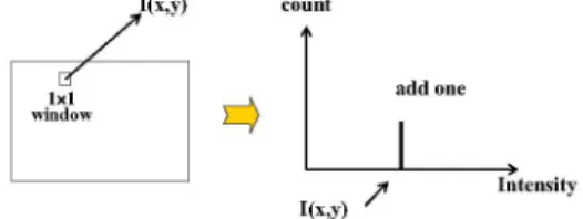
Onthe otherhand,the generationof thehistogramh(x) can

be viewed as a masking-and-accumulating operation. Imagine we use a 1x1 mask to scan through the image to measure the intensity data at each pixel. These intensity

values are then accumulatively added into h(x). By repeating the masking-and-accumulating operation over the whole image, the histogram function h(x) is obtained. In

Figure 1, we illustrate such a masking-and-accumulating operation. Due to the limited size of the 1xl mask, the HE

method doesn't consider the neighboring information around each pixel. Hence, the histogram function h(x) containsonly global statistics of theimage.

I(x,y) count Count f2(I(x,y),N(x,y)) addone fl(I(x,y),N(x,y)) \/--- ..''

(a)

(b)

Figure 2 (a) Illustration of I(x,y) and N(x,y).

(b)Generationof the extendedhistogram

addone

A

I(x,y)/21 lntensity

I(x,y)

Figure I Illustration ofhistogram generation D C B Intensity Value

2.2 Proposed Algorithm 2.2.1ExtendedHistogram

In our approach, we first extend the scanning mask size from 1x1 to nxn. When the center of the mask isplaced at

(x,y), we define I(x, y) as the intensity value at the center pixel, while define N(x, y) as the set ofintensity values within the nxn neighborhood of(x,y). The definitions of I(x,y) and N(x,y) are illustrated in Figure 2(a). Besides, we propose the use of two measures f1(I(x,y),N(x,y)) and

f2(I(x,y),N(x,y))

to estimate some local characteristics within the mask window. Here, we define f1 and f2 to

measure the local average and local variations within the mask, respectively. For example, if we choose the mask size

tobe 3x3,wemaydefine f1 andf2tobe 11 11

r(x,Y)= -L

₉

Y

I(x

+i,

y+

j)(2

i=-j=-l

f2(x)

Max{I(x+i,y+j);-l<i<1,1<j<1}

(3)

Min{I(x+i,y+ j);-l<i<1,-l<j<1}

In fact, many other functions, like aweightedmeanand the localvariance, can also be used to definef1andf2.

With the definitions of f1 and f2, we can calculate

f1(I(x,y),N(x,y))

and

f2(I(x,y),N(x,y))

ateach

pixel (x,y).

As the maskscans throughthe image, we countthe occurrence frequency of (f1,f2) and generate a so-called "extended

histogram". Figure 2(b) illustrates the generation of this extended histogram. This operation is similar to the

operationillustrated inFigure 1, except that the mask size is now nxn and the intensity value I(x,y) is replaced by two

local measures f1 and

f2.

After thegenerationof the extendedhistogram, weperform normalization over the extended histogram to get the 2-D probability density function p(f1,f2). In theory,

p(f1,f2)

records the global statistics of the local characteristics. For example,if

p(c,4)

=k, itmeans there exists somepixels in

the image with local features being fi = oc and f2

=3.

Moreover, theoccurrence rateof thesepixelsis k.

(a) P7 0 P5 0_P6 Pi P2 P3 P4 (c) Figure3 (a)Synthesized image.

(b) Histogram.

(c) p(f1,f2)

of

(a).

(b)

P8

fi

In Figure 3(a), we show a synthesized image, which contains 4 smooth regions, A, B, C, and D. The histogram

of thisimage is shown inFigure 3(b).Due tothe fact that C and D occupy only a small portion of the image, it is

expected that the contrast between C and D cannot be

adequately enhanced by the HE algorithm. In Figure 3(c), we show an illustration of the 2-D pdffunction p(f1,f2) of

Figure 3(a). Here, PI, P2, P3, and

P4

correspond to the smooth parts of A, B, C, and D, respectively. Onthe other

hand, P5,

P6,

P7and P8 correspond to the boundary regions

betweenA and B; B and C; B and D; and C andD. Here,

we use abrightercolortorepresentalargervalue ofp(f1, f2)

while use adarker colortorepresent a smaller value. It can

beeasilyseenthat this 2-Dpdffunction

p(ft,f2)

offers much more useful information than the 1-Dhistogram. Itrecords

not only the distribution of intensity values but also the

distribution of local variations. Based on

p(f1,f2),

we can easily distinguish pixels in smooth regions from pixels at boundary regions. Thiscapabilityenablesmorecomplicated manipulationsforimageenhancement.

2.2.2ExpansionFunction

Based on

p(f1,f2),

we aim to develop a suitable intensity mapping function that can satisfactorily enhance image contents. Inthis paper,weproposetheuse ofa"conditional

expansion function" to generate the intensity transfer function. This conditional expansion function

2878

/I(xy

n -E>

S[g

(f1

f2)=(a,

,6)]

is defined as a function ofintensity

value g, given fi = oc and f2 = 3. That is, this function

describes howlikely we want the intensity values around g toexpand if we are given the condition that fi =oc andf2= 3.

For example, if we want to enhance the image contrast in Figure 3(a) without enhancing image noise over smooth regions, we may simply set a threshold over f2 to screen out PI, P2, P3, and p4

first.

Onthe other

hand,

forP5,P6,P7, and

P8,

which

correspond

to

edge regions

in the

image,

we may

define the conditional expansion function to be something

like

S[g

(fi1f2)

=

(a,)]

=

f(ga)

where

HI(x)

is therectangularfunctionexpressedas

{I -0.5<x<0.5

H

(X)

-

otherwise

= 6(g-f1), then S(g) degenerates to the normalized form of

the 1-Dhistogram h(x). c +s(g) IntensityValue

(a)

(b)

T(g)

(4)

(5)

This means once we have observed a set of local statistics with fi = oc and f2= 3, then we expect theintensity values

within the range

[uc-0.5f3,c+O.5f3]

are more likely to be

expanded. Of course, there are many other choices of

S[g1f1,f2],

depending on how we want the image to be enhanced. Moreover, since the value of

p(f1,f2)

reflects the

occurrence frequencyof(f1,f2),we mayfurther take

p(f1,f2)

into account and calculate theaveraged expansion function:

s(g)

gmax

S

I(S[gf(fl,f2)]p(fl,f2)dfldf2

(6)

,imin rnin

ThisS(g) function indicates which intensity values are more

likely to be stretched in the image enhancement process. Then, based on S(g), we can deduce the intensity transfer functionT(g),which isdefinedas

[c

+

S(r)]dr-T(g)

=gj. +

(gmax -gmin)

in

mm

[c+

S(r)]d

(7)

An illustration ofS(g) and T(g) for the example ofFigure 3(c)is shown inFigure4. Here,we set athresholdoverf2to ignore

pi,

P2, P3 and

p4.

S[gf1,f2] isdefined as Equation (4)

and Figure 4(a) shows the

S[gJf1,f2]p(f1,f2)

profiles

corresponding to P5,P6, P7, andP8. Based on Equations (6)

and(7), c+S(g) andT(g) canbeeasily computed, as shown inFigure 4(b)andFigure 4(c).

It canbeeasily imaginedthat if(c+S(g)) has alarger value

at g, then T(g) has a larger slope at g. This means the

intensityvalues around g tend to be stretched more. Hence, after having obtained the expansion function S(g), we can

deduce the intensity transfer function T(g) to assign intensityvalues based ontheprominence of local statistics. Moreover, note that in Equation (7) we add one extra

parameter c. This parameter provides flexible control over

the degree of image enhancement. A smaller value of c causes a more apparent adjustment, and vice versa.

Moreover, it is worthmentioningthat ifwechoose

S[glfl,f2]

Intensity Value

(c)

Figure4 Exampleof

S[gJf1,f2]p(f1,f2),

c+S(g),andT(g). 2.2.3PreventionofOver-Enhancement

As mentioned above, once we have gotten the expansion function S(g), we can generate the intensity transfer function based on Equation (7). In practice, the magnitude

of S(g) has significant influence on the enhanced result. If there are some dominant peaks in S(g), overly enhanced

images may be produced. To avoid this problem, we proposed the use of a magnitude mapping function

MO )

to compress the dynamic range of S(g). This magnitude mapping function is a monotonically increasing function,

with itsslope monotonically decreasingto zero. Anexample

of

MO

is

Y=M(X)=

X1XM°

(8)

where X is the original expansion function, Y is the

adjusted expansion function, and

Mo

isa control parameter.

Insummary,Equation (7)is furthermodifiedtobe

,[c

+

M(S(-r))]d-c

T(g)=

gmin

+

(gmax

-gmin)

L[in (9)

[c

+

M(S(r))]drc

With the use of

M(

), the expansion function with large magnitudeswill beproperly constrained to an extent so that theprocessed imagelooksmorenatural.

3. APPLICATIONS 3.1 ContrastEnhancement

In our simulations, an RGB-formated color image is first

converted to the HSI color space and we apply our algorithm to the I component only. Besides, f1 and f2 are defined as Equations (2) and (3). To perform contrast enhancement,wedefine

S[glfl,f2]

as

,>I10 otherwise

InFigure 5, weshowsomesimulations and the comparisons with HE, AHE and the method proposed by [3]. We can

find that the proposed algorithm provides robust and more natural enhancement results. Besides, it is worth mentioning that the image quality in Figure 5(d) is with little improvement due to the mean-preserving constraint used in [3], Moreover, eventhough there exists strong image noise in Figure 6(a), we may still properly enhance the image contrastwithoutoverly enhance the image noise.

(a)

(d)

(e)

Figure 5. (a) Original image. (b) HE. (c) AHE. (d) Processed result of [3]. (e) Proposed method(C=0,Mo=2).

(a) (b) (c)

Figure6.(a) Original imagecontaminates with Gaussian noise.

(b)HE.(c) Proposedmethod(C=0,Mo=2).

3.2 Shadow Enhancement

The luminance variation within a scene often has a very wide dynamic range.Due to the narrowerdynamic rangeof the capturing devices, some portions of the reproduced image may look too dark or toobright. In this section, we demonstrate how theproposed method canbe used to deal with the shadow enhancementproblem.

For shadow enhancement, we may enhance areas with

smallergradientswhile suppress areaswith larger gradients.

This concept was proposed by [6] for dynamic range

compression. To achieve the same goal, here we may redefine the conditionalexpansionfunction to be

S[g

(fl,f2)

=

(a,)]

-

k(8)(

a)

(11)

where

k(f)

islarge for small f, and viceversa. To suppress

image noise,wemay also set

k(f)

tobe zero iff is smaller than apre-determinedthreshold. Some experimental results

ofshadow enhancement are shown in Figure 7. It can be

seenthat dark regions areeffectivelyenhanced. 4. CONCLUSIONS

In this paper, we propose a new approach for image enhancement. In this approach, we extend the concept of histogram equalization to record the global statistics of

some local characteristics. A complete procedure for the generation of the intensity transfer function is developed. Experimental results demonstrate that the proposed approach can provide a reliable and flexible scheme for variousimage enhancement applications.

(a)

(b)

(c) (d)

Figure 7. (a) (c): Original images.(b)(d): Images enhanced by the

proposedmethod.(c=0,MO=2)

ACKNOWLEDGEMENT

This research was supported by National Science Council of the Republic of China under Grant Number NSC-93-2219-E-009-017.

4. REFERENCES

[1]R.C. Gonzalez and R. E.Woods, Digitalimage processing, Addison-Wesley, 2002.

[2] Y.T. Kim, "Contrast enhancement using brightness- preserving

bi-histogram equalization," IEEE Trans. on Consumer

Electronics,Vol. 43, No. 1, pp.1-8, Feb. 1997.

[3] Soong-DerChen,Abd. RahmanRamli, "Minimum mean

brightness error Bi-histogram equalization in contrast

enhancement,"IEEETrans. on ConsumerElectronics,Vol. 49, No.4, pp.1310-1319, Nov. 2003.

[4] J.Y. Kim, L.S. Kim and S.H. Hwang, "An advanced contrast enhancement using partially overlapped sub-block histogram equalization,"IEEETrans. on Circuitsand Systemsfor Video

Technology, Vol. 11,Issue4, pp.475-484,Apr. 2001.

[5] T.K. Kim, J.K. Paik and B.S. Kang, "Contrast enhancement system using spatially adaptive histogram equalization with

temporal filtering,"IEEETrans. onConsumerElectronics,Vol. 44, Issue 1, pp.82-87,Feb. 1998.

[6]R.Fattal,D.Lischinski and M. Werman, "Gradient domainhigh dynamicrangecompression",Proc.ACMSIGGRAPH'02

2880

I

lyg-a)

S[g

(fl,f2)

=

(a,,g)]

=-

18