A Study on the Optimization Methods for Optomechanical Alignment
Ming-Ta Yu
a, Tsung-Yin Lin
b*, Yi-You Li
a, and Pei-Feng Shu
aa
Dept. of Mech. Eng., National Chiao Tung University, Hsinchu 300, Taiwan, R.O.C.
bDept. of Mech. Eng. Chung Cheng Institute of Technology, NDU, Taoyuan 335, Taiwan, R.O.C.
ABSTRACT
The alignment for optomechanical components is important in designing and manufacturing optical systems. This study uses optical fibers for example to find suitable optimization strategies for optomechanical alignment. The core diameter of the single-mode fiber is about 6µm to 9µm. Any slight misalignment or deformation of the optical mechanism will cause signification optical losses during connections. The alignment methods can be divided into passive and active ones. In the passive alignment, optical connectors, ferrules, and sleeves are used to align two optical fibers. In the active alignment, the best connection position with minimum connection losses must be found, and users usually take a lot of effort to do this. This study uses different optimum methodologies: non-gradient-based, gradient-based, and Hessian-based methods, to find the optimum position. The non-gradient-Hessian-based method has low accuracy and the efficiency cannot be increased. The gradient-based methods seem to have better efficiency to find the optimum position because it uses gradient information to calculate the search direction in every iteration. Finally for the Hessian-based methods, it is found that the advantage of using Hessian matrix is not obvious because the light intensity distribution is similar to the Gaussian distribution.
Keywords: optimization, optical fiber, optomechanical alignment.
1. INTRODUCTION
Fiber optic communications with low loss and broadband characteristics developed quickly after low-loss fibers were introduced in 1970. Because of the high capacity, high transmission rate, and no electromagnetic interference during optical communications, optical fibers have been steadily replacing copper wire as an appropriate means of signal transmission in recent years.
Similar to other communication mediums, optical fibers do not have infinite length. Fibers should be aligned and connected to each other when building the optical fiber network. Methods used to align fibers can be divided into passive and active methods. The passive methods use optical connectors and mechanisms to align and joint fibers. But the core diameter of a single-mode fiber is about 6µm to 9µm. Any slight misalignment or deformation on the connecting mechanism will cause signification optical losses across connections. Therefore, the design of the passive component is very important, and high manufacturing precision is required to make the component.
On the other hand, the active method will search the optimum position with the least transmission loss actively, and connect fibers in this position. It can ensure the connection performance of the two connecting fibers, but the time required for searching optimum position will increase the working-hours of component manufacturing. It will be unpractical if the time of searching optimum connection position is too much. Therefore, how to find the optimum connection position efficiently is the main objective in the active alignment method.
The optical fiber alignment problem is a typical unconstrained optimum design problem. This optimum design problem adjusts the connection position to find the position with the maximum light intensity or minimum optical power loss. Therefore, the objective function is the light intensity and the design variables are the coordinate values of the connection position. There is no constraint in the fiber alignment problem unless the coordinate values of connection position, and the boundaries are not treated as constraints in the optimum design problem. The typical solving process of this optimum design problem is called a “searching process”, and it can be divided into two parts: finding search directions, and finding the step size along the determined search direction. The detail solving process will be explained in the next section.
In 2001, Tang, et al.1 used Hill-climbing Method to solve the alignment problem to find the optimum connection
position. Mizukami, et al.2 simulated the alignment process as the equations of Hamiltonian Algorithm and solve the
equations to find the position with maximum light intensity. Pham and Castellani3 simulated the searching process as
moving in the light intensity surface to avoid the trap of local minimum, and solve the problem with gradient-based method. Chang and Chen4 used the predetermined search direction and used Swann’s Method and Quadratic Estimation
Method to find the step size. In 2002, Siao and Li5 used Gaussian Function to estimate the light intensity in the search
direction. In 2003, Zhang and Shi6 used Matlab/Simulink to solve Hamiltonian Algorithm to find the optimum
connection position. Sung and Huang7 used Steepest Descent Method to calculate the search direction and used Golden
Section Search to find the best step size. They also used Coordinate Search Method and Pattern Search Method to search the optimum connection position in the design space directly. In 2004, Zhang and Shi8 used Simplex Method to solve the
fiber alignment problem. Chen et al. 9 used a novel Simplex Method to avoid the trap of local minimum. Sung and Chiu10
used Genetic Algorithm to find the global optimum connection position and used Hill-climbing Method to improve the solution found with Genetic Algorithm.
Coordinate Search Method, Pattern Search Method, Simplex Method, and Genetic Algorithm search the optimum solution in the design space directly and they are non-gradient-based method. They do not calculate the search direction and the efficiency will not good if the design space is large. The Hill-climbing Method used in the above literatures does not calculate the search direction, too. The optimum solution is searched in predetermined directions. Typically, the directions along with X and Y axis will be used repeatedly. The efficiency is limited because the directions along X and Y axis may not be the direction with maximum increase of the light intensity. Swann’s Method, Quadratic Estimation Method, Gaussian Function Estimation, and Golden Section Method are used to calculate the step size and they have to be used with a direction searching method, such as Steepest Descent Method. There are few direction searching methods used in the optical fiber alignment problem. This study will introduce some direction searching methods that can be used in the fiber alignment problem and compare the efficiency between them and Genetic Algorithm.
2. METHODS FOR SOLVING OPTIMUM DESIGN PROBLEMS
The optimum design model will be formulated as finding the solution with minimum objective function value. This formulation can also consider the problem of maximizing the objective function value by multiplying the objective function with minus 1. The Methods used to solve unconstrained optimum design problems can be divided into indirect methods and direct methods. Indirect methods are analytic methods. They solve the necessary condition first and check the sufficient condition of an optimum design problem. The necessary condition of an unconstrained optimum design problem is the components of the gradient vector of the objective function have to be zero, and the sufficient condition is the Hessian matrix of the objective function has to be positive definite. Indirect methods can get the exact and global optimum solution, but they need the explicit function between objective function gradient and design variables. Unfortunately, it is difficult to find the explicit function of the light intensity because the light intensity has to be detected on every position. Therefore, the indirect methods can not be used to solve the fiber alignment problem but the direct methods can. Direct methods are numerical methods, and they solve an optimum design problem by “searching”. It can be described by the following iterative prescription:
; ) ( ) ( ) 1 (k X k X k X + = +∆ k=0, 1, 2… (1)
where X(k) is the collection of design variables with vector form and the superscript notes the iteration number. ΔX(k) is
the step from the solution of iteration k to iteration (k+1), and it is also a vector form. The step should be decided to improve the design. How to decide it is the main objective of solving methods. The step can be described by a “search direction” and a “step size” and it can be shown as follows:
; ) ( ) ( ) ( ) 1 (k X k k dk X + = +α k=0, 1, 2… (2)
where d(k) is the search direction, and α(k) is the step size (scalar). Thus, the solving process can be divided into solving
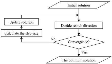
two subproblems: how to decide the search direction and how to decide the step size. The whole solving process is shown in Fig. 1. In the beginning, an initial solution X(0) should be selected, and it is the starting point of whole process.
The search direction d(k) will be decided in the second step. There are many methods for determining the search direction
and some popular methods will be introduced latter. Before moving along the search direction, the convergence condition of the process should be checked. The common convergence condition is that the gradient norm value of the
but the norm is difficult to be zero when using numerical methods. Therefore, a predetermined small value is used instead of zero. Another common convergence condition is checking the difference of objective function values between two solutions, and the solving process will stop if the difference is less than a predetermined small value. It means it is not efficient to continue solving process for the small improvement of the objective function. The solving process will continue if the convergence condition is not satisfied.
The step size along the search direction will be calculated if the solving process continues. The process of calculating the step size usually called “one-dimensional search” because it search optimum solution “along” the search direction. Hence, it becomes a one-dimensional problem in the step size calculating process no matter how many the dimension of the problem is. There are also many methods for the one-dimensional search in literatures as introduced above. This study only applied one method: the Golden Section Method11 for calculating the step size because it is not the main
object in this study. After determining the search direction and the step size, the solution can be updated, and it can continue to the next iteration.
Fig. 1. The solving process of direct methods
There are many methods for deciding search direction, such as Steepest Descent Method, Conjugate Gradient Method, DFP (Davidon-Fletcher-Powell) Method, and BFGS (Broyden-Fletcher-Goldfarb-Shanno) Method. The front two methods are gradient-based methods and the others are Hessian-based methods. They will be introduced in following sections.
2.1 Gradient-based methods
Taylor’s series expansion for f(X) about the point X(k) is:
1 ) ( ) ( ) ( ) ( ) ( ) (X f X c X X R f = k + k ⋅ − k + (3)
where c(k) is the gradient vector of f(X) at point X(k) and R
1 is the remainder term. Using Taylor’s series expansion to
approximate f(X) by ignoring the remainder term, and substitute X(k+1) of equation (2) for X. The equation (3) becomes:
) ( ) ( ) (X(k 1) f X(k) c(k) (k)d(k) f + = + ⋅α (4)
The model is formulated as finding the solution with minimum objective function value. Therefore f(X(k+1)) should be
less than f(X(k)) if the design is suitable for updating.
0 ) ( ) ( ) (X(k+1) − f X(k) = (k) c(k)⋅d(k) < f α (5)
Thus, any d(k) satisfies equation (5), i.e. the angle between d(k) and c(k) is between 90 degree and 270 degree, can be the
search direction and the gradient-based methods use this concept to decide their search directions. Initial solution
Decide search direction
Convergence? Calculate the step size
The optimum solution Update solution
Yes No
2.1.1 Steepest Descent Method
The gradient vector at a point X indicates in the direction of maximum increase in the objective function. The Steepest Descent Method uses the direction of maximum decrease in the objective function as its search direction. Thus it uses the direction that is opposite to the gradient vector. It can be shown as:
) ( )
(k ck
d =− (6)
2.1.2 Conjugate Gradient Method
Steepest Descent Method uses the simplest way to decide the search direction, but it is usually not efficient in general case because search directions of two continuous iterations in Steepest Descent Method are orthogonal to each other. Therefore, there are many methods to modify the search direction of Steepest Descent Method, and Conjugate Gradient Method is one of them. Conjugate Gradient Method adds the information of the last search direction to this search direction to improve the efficiency. It can be shown as:
) 1 ( ) ( ) ( ) (k =−ck + kd k− d β k=1, 2, 3… (7) where 2 ) 1 ( ) ( ) ( ⎟ ⎟ ⎠ ⎞ ⎜ ⎜ ⎝ ⎛ = − k k k c c β k=1, 2, 3… (8)
The first search direction is:
) 0 ( ) 0 ( c d =− (9)
At the first search direction, it is the same as the Steepest Descent Method because no last search direction can be used. Thus, the first two solutions of them will be the same.
2.2 Hessian-based methods
Taylor’s series expansion for the objective function f(X) at the point X(k) can be expressed in detail: 2 ) ( ) ( ) ( ) ( ) ( ) ( ( ) ( ) 2 1 ) ( ) ( ) (X f X c X X X X H X X R f = k + k ⋅ − k + − k T k − k + (10)
where H(k) is the Hessian matrix of the objective function at point X(k) and R
2 is the remainder term. Ignore the remainder
term, equation (10) can be simplified as:
X H X X c X f X f = (k) + (k)⋅∆ + ∆ T (k)∆ 2 1 ) ( ) ( (11)
The optimum design problem becomes finding ΔX that causes minimum f(X). As solving it with analytic methods, set the first differential equation equal to zero and solve it.
0 ) ( ) ( = ( )+ ( )∆ = ∆ ∂ ∂ X H c X X f k k (12) Then, ∆X =−H(k)−1c(k) (13)
It can be used as the search direction in the iteration k. These kinds of methods are called Hessian-based methods because they use the Hessian matrix of the objective function to decide the search direction. Using equation (10) to approximate f(X) is more accurate than using equation (3). Thus, the searching will be more efficient in general case. For some applications, calculating Hessian matrix may be tedious or even impossible, and sometimes the Hessian matrix will be singular. Therefore, some methods overcome these drawbacks by generating an approximation for the Hessian matrix and its inverse.
2.2.1 DFP Method
DFP Method [11] generates an approximate inverse of the Hessian matrix of f(X). Its search direction is shown as follows: ) ( ) ( ) (k Akck d =− (14) where A(k+1) =A(k)+B(k)+C(k) (15) ) ( ( ) ( ) ) ( ) ( ) ( k k k k k y s s s B T ⋅ = (16) ) ( ( ) ( ) ) ( ) ( ) ( k k k k k z y z z C T ⋅ − = (17) ) ( ) ( ) (k kd k s =α (18) ) ( ) 1 ( ) (k ck ck y = + − (19) ) ( ) ( ) (k Ak yk z = (20)
A(0) is set as the identity matrix at beginning.
2.2.2 BFGS Method
BFGS Method11 generates an approximation of the Hessian matrix of f(X). Its search direction is shown as follows: ) ( 1 ) ( ) ( k k A k H c d =− − (21) where ( ) (k) (k) (k) A k A H D E H = + + (22) ) ( ( ) ( ) ) ( ) ( ) ( k k k k k s y y y D T ⋅ = (23) ) ( ( ) ( ) ) ( ) ( ) ( k k k k k d c c c E T ⋅ = (24)
HA(0) is set as the identity matrix at beginning.
2.3 Non-gradient-based method
Genetic Algorithm is used to solve the optimum design problem in many applications because it is suitable for different problem, such as discrete design variable problem and the problem that the objective function gradient can not be calculated, because it does not use the gradient information of the problem. Its solving process is much different from gradient-based methods and Hessian-based methods. At beginning, it generates many individuals, i.e. solutions, randomly and these individuals are called a generation. The individual number is called the population size. The objective function value of every individual will be calculated, and the individual has a good objective function value will has high probability to generate individuals of the next generation. The operators used to generate new individuals are called crossover and mutation12. These operators simulate the propagation process in the nature and this is the reason
why it is called the “genetic” algorithm. The solving process will be stopped when the predetermine generation number is complete, and the best individual of all is the optimum solution of Genetic Algorithm.
3. RESULTS AND DISCUSSION
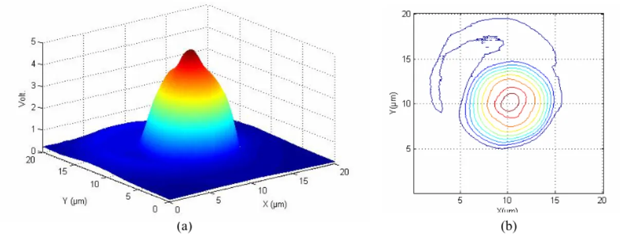
The real light intensity detected by the equipment is transferred to voltage as shown in Fig. 2(a), and Fig. 2(b) shows the light intensity contour.
6 ID ID 20 XIuml
Volt
Fig. 2. (a) Light intensity (b) light intensity contour
The center circles are the light intensity in the fiber with 9μm diameter. The light intensity will multiply minus 1 later because the optimum design problem is formulated as finding the minimum objective function value. Before starting to search the optimum connection position, fibers will be aligned roughly first and the rough alignment may be on any side to the optimum connection position. Thus, cases with different points will be used as initial solutions in the solving process. The case I uses (X, Y) = (8, 10) as the initial point, and the case II uses (X, Y) = (10, 8) as the initial point. The results are shown in Table 1.
Table 1. (a) Data of case I (b) data of case II
The “function calls” is the number of calculating the objective function value and they usually cost most of the time in the solving process. Thus, it can be used to evaluate the efficiency of solving methods. But the iteration number will be better used when comparing the direction searching methods because the function calls depends on not only the direction decision but the one-dimensional search process.
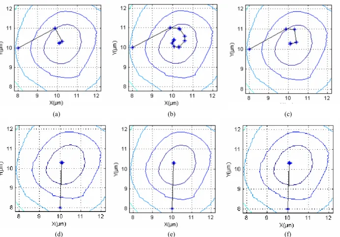
The iteration number of Conjugate Gradient Method is the same as Steepest Descent Method in case II, but they are very different in case I. In case I, the search direction of Steepest Descent Method in iteration 1 points to the optimum solution closely, as shown in Fig. 3(a), and the norm of the objective function gradient of iteration 1 is larger than iteration 0, as shown in Table 2. Therefore, the β(1) is large and the effect of the last search direction is also large when
using Conjugate Gradient Method. Thus, the search direction will not point to the optimum solution and the efficiency will be reduced, as shown in Fig. 3(b). In case II, the initial point of iteration one is close to the optimum solution and the objective function norm is small, as shown in Table 2. Therefore, the β(1) is small, and the Conjugate Gradient Method
degenerates to Steepest Descent Method, as shown in Fig. 3(d)(e).
(a) (b)
(a)
Case I Function calls Iteration number Objective function value
Steepest Descent Method 505 4 -4.892
Conjugate Gradient Method 1045 11 -4.889
DFP Method 504 5 -4.892
BFGS Method 398 5 -4.892
(b)
Case II Function calls Iteration number Objective function value
Steepest Descent Method 324 3 -4.892
Conjugate Gradient Method 324 3 -4.892
DFP Method 276 3 -4.892
6 9 10 11 12 X(IJm) 6 9 10 11 12 X(IJm) 6 9 10 11 12 6 9 10 X(IJm) 11 12 6 9 10 11 12 X(IJm) 12 11 10 2-9 a 6 9 10 X(IJm) 11 12
Fig. 3. Searching pass of solving methods (a) Steepest Descent Method in case I (b) Conjugate Gradient Method in case I (c) DFP Method in case I (d) Steepest Descent Method in case II (e) Conjugate Gradient Method in case II (f) DFP Method in case II
Table 2. Objective function norms of Steepest Descent Method and Conjugate Gradient Method
With the similar reason, the search direction of DFP Method will be modified far from the Steepest Descent Method’s, as shown in Fig. 3(c), by approximate inverse Hessian matrix in case I and the efficiency will be decreased.
The Genetic Algorithm is also used in this study and the results are shown in Table 3.
Table 3. Results of Genetic Algorithm
The population region is set as a square and it is from (X, Y) = (80, 80) to (120, 120). The total individual number is set as 400 because the function calls in case I and case II are about 300 to 500. The results of Genetic Algorithm are not better than the results of gradient-based methods and Hessian-based methods, but they are good enough because the differences are less than 0.3%. Although the Genetic Algorithm is workable, it is difficult to enhance the efficiency of
||c(0)|| ||c(1)|| β(1) Case I 0.044 0.073 2.705 Case II 0.076 0.007 0.008 (a) (b) (c) (d) (e) (f)
Objective function value of the best individual Population size Generation
First time Second time Third time
40 10 -4.883 -4.879 -4.890
20 20 -4.884 -4.890 -4.890
Genetic Algorithm. On the contrary, enhancing the efficiency of gradient-based methods and Hessian-based methods is easily. As shown in Table 1, the solving process only has about 4 iterations and it means most function calls are happened in the one-dimensional search. Thus, enhancing the efficiency of the one-dimensional search is helpful for enhancing the efficiency of the fiber alignment.
4. COLCLUSIONS
The core diameter of the single-mode fiber is about 6µm to 9µm. Any slight misalignment or deformation of the optical mechanism will cause signification optical losses during connections. The optical fiber alignment problem is a typical unconstrained optimum design problem. This study uses different optimum methodologies: non-gradient-based (Genetic Algorithm), gradient-based (Steepest Descent Method and Conjugate Gradient Method), and Hessian-based methods (DFP Method and BFGS Method), to find the optimum position. Therefore, conclusions can be summarized as follows: 1. The iteration number of Steepest Descent Method is small because the light intensity distribution is similar to
Gaussian distribution.
2. The Steepest Descent Method is better in the alignment problem because the iteration number is small and any modification of the gradient information will let the search direction far from the optimum point.
3. A good one-dimensional search method is important in the fiber alignment problem because the iteration number of solving process is small and most function calls are happened in the one-dimensional search.
4. Genetic Algorithm is suitable for the fiber alignment problem but it is difficult to enhancing the efficiency.
ACKNOWLEDGEMENT
The support of this research by the National Science Council, Taiwan, R.O.C., under grant NSC94-2212-E-014-002 is gratefully acknowledged.
REFERENCE
1. Z. Tang, R. Zhang, and F. G. Shi, "Effects of angular misalignments on fiber-optic alignment automation," Opt. Commun. 196, 173-180(2001).
2. M. Mizukami, M. Hirano, and K. Shinjo, "Simultaneous alignment of multiple optical axes in a multistage optical system using Hamiltonian algorithm," Opt. Eng. 40(3), 448-454(2001).
3. D. T. Pham and M. Castellani, "Intelligent control of fiber optic components assembly," Proc. Instn. Mech. Engrs. 215, 1177-1189(2001).
4. B. R. Chen and S. H. Chang, Development of Fiber Auto-alignment Fabrication Technology, thesis, Taiwan University, Taipei, 2001.
5. S. J. Siao and M. E. Li, Nonlinear Regression Analysis for Fiber Alignment, thesis, Kaohsiung Normal University, Kaohsiung, 2002.
6. R. Zhang and F. G. Shi, "Novel fiber optic alignment strategy using Hamiltonian algorithm and Matlab/Simulink," Opt. Eng. 42(8), 2240-2245(2003).
7. M. Y. Sung and S. J. Huang, Application of Piezoelectric-actuating Table in Optical Alignment, thesis, Taiwan University of Science and Technology, Taipei, 2003.
8. R. Zhang and F. G. Shi, "A novel algorithm for fiber-optic alignment automation," IEEE Trans. Adv. Packag. 27(1), 173-178(2004).
9. P. H. Sung and S. H. Chiu, The Study of the Fiber-optic Automatic Alignment Using Genetic Algorithm with Hill-climbing Algorithm, thesis, Taiwan University of Science and Technology, Taipei, 2004.
10. W. S. Chen, C. Y. Tseng, and C. L. Chang, The Study of Automation Method for Multi-degree-of-freedom Fiber-optic Alignment, thesis, Ping Tung University of Science and Technology, Pingtung, 2004.
11. J. S. Arora, Introduction to Optimum Design, McGraw Hill, 1989.