右方設限長期存活資料比率之研究

(1)

右方設限長期存活資料比率之研究

蘇秀媛

1

_{*、蘇志雄}

2

_、謝鑫能

1 1

_{國立臺灣大學農藝學系}

2

_{致理技術學院會計學系}

摘要

自從

Boag (1949)提出「治癒資料」的

分析方法後，部分學者將此方法成功的應用

在醫學資料的分析。本篇文章稱

Boag 所提

的「治癒資料」為「長期存活資料」，亦即

在存活資料中，若實驗期間能無限延長下，

有部份資料都能永久存活。對於此類資料，

我們延用

Boag 的方法，定義在右方設限資

料下概度函數，並假設存活母體為指數分布

與

Weibull 分布，導出「長期存活資料」比

率之最大概度估計式及概度比檢定，同時利

用

Kaplan and Meier 的估計方法，提出無

母數方法來估計「長期存活資料」比率及檢

定方法。本文利用蒙地卡羅統計模擬方法比

較在最大概度法及無母數方法不同情形

下，觀察「長期存活資料」比率的狀況，發

現在中、低設限下，無母數方法在檢定「長

期存活資料」比率的檢定力優於最大概度

法。

關鍵詞︰治癒資料、長期存活資料、右方設限、

蒙地卡羅統計模擬、最大概度法。

The Proportion of Long-term Survivor

Data in Right Censored Case

Hsiu-Yuan Su

1

_{*, Chih-Hsiung Su}

2

_and

Hsin-Neng Hsieh

1

1 _{Department of Agronomy, National Taiwan} University, Taipei 106, Taiwan (ROC)

2 _{Department of Accounting , Chihlee Institute of} Technology, Banciao, Taipei Hsien 220, Taiwan (ROC)

ABSTRACT

Since the method for analyzing the cured data was proposed by Boag in 1949, it has been applied to many medical data successfully by other scholars. The “cured data” in Boag’s paper was renamed as “long-term survival data” here. The long-term survival data means some of the data can survive in indefinite time. The likelihood function with right-censored data was defined by using Boag’s method. The survival population was assumed to be exponential distribution or Weibull distribution. The MLE (maximum likelihood estimator) and LRT (likelihood ratio test) can be derived for long-term survival data. Furthermore, a nonparametric method for estimating proportion of long-term survival data was derived based on Kaplan-Meier’s estimation. In this paper, we compare the MLE and non-parametric method by Monte Carlo simulation method for long-term survival data. We find that the performance of non-parametric test is better than that of maximum likelihood ratio test in cases of middle censored rate and low censored rate.

Key words: Cured data, Long-term survivor data, Right-censored, Monte Carlo simulation, Maximum likelihood ratio test.

* 通信作者, suwong@ccms.ntu.edu.tw 投稿日期：2004 年 4 月 10 日

接受日期：2004 年 7 月 14 日

作物、環境與生物資訊 2:95-104 (2005) Crop, Environment & Bioinformatics 2:95- 104 (2005) 189 Chung-Cheng Rd., Wufeng, Taichung Hsien 41301, Taiwan (ROC)

(2)

前言

影響種子發芽成功之因素，包括溫度、

水分、陽光、品種、繁殖地區等。為了描述

種子發芽過程，前人研究利用不同的分布來

描述種子發芽的表現，部分學者利用數學函

數型態來描述上述種子累積發芽率之發芽

過程：如常態分布函數

(Butterworth and

Janssen 1973)、Gamma 分布函數(Thornley

1977)、Weibull 分布函數(Brown 1987)等。

這些分布中以

Weibull 分布函數來描述種

子發芽過程較其他分布合適，而且

Weibull

分布函數之參數亦具有生物上之意義

(Brown 1987, Bahler et al. 1989, Dumur et

al. 1990, Huang et al. 1995, Su et al. 2000,

2003)。但是 Weibull 分布函數估算參數的

方法複雜，利用不同的數值方法，或給定不

同的起始值，都可能估計出不同組的解，因

此在應用上並不方便。

有關種子發芽行為的研究中，學者皆利

用數學函數做為分析基礎，本文利用統計之

假設檢定，透過存活分析

(survival analysis)

的統計方法，建立種子發芽比率的統計推

論。由於種子發芽試驗是有其時間限制，所

以在試驗期間內不見得所有的種子皆能發

芽完成，而未發芽完成的種子亦有資訊，表

示其發芽成功所需的時間至少超過試驗期

間，故將此類種子發芽時間視為統計上一組

第

I 類型的右方設限存活資料(typeＩright

censored survival data)。而因有些種子可

能永遠都無法發芽成功，在本文中將此種資

料稱之為『右方設限長期存活資料（

right

censored long-term survivor data）』

。透過

存活分析的統計方法，來建立種子長期存活

資料的發芽比率之統計推論。

前人研究及相關分析工具

1.前人研究

長期存活資料(Maller and Zhou 1996)

指在整個存活時間分布具有長久存活之個

體存在，若

_F

_T

_(t

₎

為存活時間之累積分布函

數

(cumulated distribution function)，則通

常

_F

_T

₍

∞

₎

=

₁

，但若擁有長期存活資料時，

則

FT(∞)=p，　0<p<1

，而

1 −

p

即為母體中

之長期存活資料比例，又稱免疫比例

(immune proportion)。

Boag (1949)是最早提出「長期存活資

料」統計分析的學者(Boag 稱「長期存活資

料」為「治癒資料」)。Boag 利用英國某醫

院中

121 名乳癌病患(1929-1938)，記錄這 9

年來接受治療後存活時間，但

9 年後仍有存

活之病患，Boag 認為此資料不能完全視為

設限資料，亦有可能屬於被完全治癒之病

患。由於

Boag 先利用卡方適合度檢定，認

為存活時間

lognormal 分布較指數分布適

合，因此提出一混合模型

(mixed model)，

其對數概度函數為：

{

}

1 2,3 4

logL log(pZ) log (1 p) pq logpq

σ = =

∑

+

∑

− + +

∑

l

其中

1 122_{, (}log _), _,₁ 2 t Z e χ q Zdx p χ μ χ σ π − − ∞ = = =

_∫

−

為被治

癒比例；

∑

1

：表示在期間內確定是因該癌

症死亡者；

∑

2

：表示在期間內確定不是由

於該癌症導致死亡者；

∑

3

：表示在期間後

仍存活仍接受該癌症影響；

∑

4

：表示

在期間後仍存活確定不受該癌症影響。並導

出最大概度估計量。

Haybittle (1965)利用指數型態來表示

『被治癒』之比例

₁

−

_p

=

_c

=

_e

−βk

_{，推導出}

Gompertz 模式，其對數概度函數為：

(

_{) ∑}

∑

+

=

2 , 1 1

log

~

log

L

q

_T

Z

_T

P

_T

l

其中

；

P_T

表示經過

(3)

第一次治療後經過

T 時間之存活比例；

P~_T

表示

正常存活母體經過

T 時間後之存活比例。

Haybittle 利用最大概度估計法推估 c,β，但並

沒有直接檢定

c 之值，只是估算出其標準誤差

(standard error)。

Goldman (1984)引用指數分布作為存

活時間之分布，建立混合模式，其對數概度

函數定義為：

[

]

(

)

log log log log ti 1

i u c L d p λ λ t pe−λ p = = + −

∑ ∑

+ + − l

其中

d

表示完整觀察之個體數；

1−p

表治

癒比例；

∑

u

表完整觀察到之個體（非設限

資料）

；

∑

c

表設限資料之個體。並分析一組

33 個攝護腺癌病患 (1973-1979) 之存活時

間，及利用蒙地卡羅模擬，發現其最大概

度估計量

ˆp

具有不偏的性質。

Farewell (1977)利用 Logistic 函數做為

共變數

之連結函數(link function)，成為

B e r n o u l l i 分布「發生」之機率（即

）

，並假設存活時間服從指

數分布，討論實驗設限時間及

Pr

(

Y=1

)

大小

對該混合模式之效率。Farewell (1982)引用

相同觀念，但將存活時間改成

Weibull 分

布，分析魚在不同的鋅含量中其存活時間之

差異。

Gordon (1990)提出在一組資料中有兩

種可能的致命因素，觀察樣本資料上可以明

確判定是屬於何種因素致命，

Gordon 做一

假設對某種特定因素來作分析時，將所有病

人區分為兩個部分，一部份為未治癒組與另

一部份皆視為治癒組。並提出混合式

Gompertz 分布，並提出其對數概度函數

為：

其中

δ₀

、

δd

、

δc

都是指標函數，分別

代表是否為其他因素致命、該疾病因素致命

及是否為設限資料，而

0 f

、

S0

、

fd

、

Sd

分

別表示為其他因素致命與該疾病因素致命

之機率密度函數及存活函數。利用最大概度

估計法估計參數並予以分析。

2.相關分析工具

(1)存活分析之數學函數

假設存活時間

T 為連續型之隨機變

數，則可定義幾個重要之函數如下：

(i) 存活機率密度函數 (probability density

function)：

0

(

)

( )

lim

, 0 .

T

P t

T

t

f t

t

ε

→

< < +

=

≥

(ii)存活累積分布函數(cumulated distribution

function)：

0

( )

(

)

t

( )

, 0 .

T r T

F t

=

P T

≤ =

t

∫

f u du t

≥

(iii)存活函數(survival function)：

( ) ( ) ( ) 1 ( ), 0 . T r _t T t S t =P T≥ =t

∫

∞f u du= −F t t≥

(iv)故障函數(hazard function)：

0

(

|

)

( )

lim

( )

, 0 .

( )

r T T T

P t

T

t

T

t

h t

f t

t

S t

ε

→

< < +

>

=

≥

(2)存活函數

S_T(t)

之估計

Kaplan and Meier (1958) 利用 PL

(product limit)的無母數方法，提出存活函

數之估計式：

(4)

其中

j n

表示存活時間

t_j

前確定存活之

個數，

j d

表示存活時間

t_j

前之「發生」之個

數，並利用

Greenwood 法則推導出

S

ˆ t

_T

(

)

之

估計標準誤：

{

ˆ

}

. .

T

( )

S E

S

t

1

( )

(

)

k j T j k j j

d

S t

n n

d

=

−

∑

長期存活資料比例之推論

假設存活時間為

T

，其機率密度函數為

0 ), (t t≥ f_T

，存活函數為

S_T(t), t≥0

，長期存

活資料比例為

S_T(∞)=1−p, 0<p<1

。

1.有母數方法

(1) 當長期存活資料為右方設限資料且母體為

指數分布(Exponential

(

λ )

)

若

. . . ( )

~

i i d i T Expλ

，設限指標函數為：

⎩ ⎨ ⎧ = ₀1_, ,完整資料_設限資料 i

δ

，

i=1,2,...,n。

則該組資料之機率密度函數為：

f

T

(t)=λe

-λt

，

t≥0

存活函數為：

S

(

t

)

=

e

−t

,

t

≥

0

T λ

_，

S

T

(t)=e

-μ

，

t≥0

概度函數為：

(

)

{

}

1 1 , i i 1 i n i i t t L λ p p λe λ δ pe λ p δ = − − − ⎡ ⎤ ⎡ ⎤ =

∏

_⎣ ⋅ _{⎦ ⎣} + − _⎦

對數概度函數為：

∑

∈ − ∈ + − + + − = c i u i p pe t p ti i) log( 1 ) log (log

λ

λ λ

參數向量為：

(i) 之點估計：

其中

。利用

Newton-Raphson 數值

方法可求得近似解

( )。

(ii) 之共變數矩陣(covariance matrix)之估

計：

⎥ ⎥ ⎥ ⎥ ⎦ ⎤ ⎢ ⎢ ⎢ ⎢ ⎣ ⎡ ∂ ∂ ⎟⎟ ⎠ ⎞ ⎜⎜ ⎝ ⎛ ∂ ∂ ∂ ∂ ⎟ ⎠ ⎞ ⎜ ⎝ ⎛ ∂ ∂ ∂ ∂ ∂ ∂ = 2 2 2 2 ) ( ) ( ) ( ) ( p p p U λ λ λ λ λ λ λ

其中

) , ( ) 1 ( ) 1 ( ) ( 2 11 2 2 2 2 p A p pe t e p p n c i t i t u i i λ λ λ λ λ = ⎥ ⎦ ⎤ ⎢ ⎣ ⎡ − + − + − = ∂ ∂

_∑

∈ − − λ ) , ( ) ( ) 1 ( ) ( 2 A12 p p p pe t e p ic t i t i i λ λ λ λ λ = ⎟⎟ ⎠ ⎞ ⎜⎜ ⎝ ⎛ ∂ ∂ ∂ ∂ = ⎥ ⎦ ⎤ ⎢ ⎣ ⎡ − + − = ⎟ ⎠ ⎞ ⎜ ⎝ ⎛ ∂ ∂ ∂ ∂

_∑

∈ − − _λ λ ) , ( ) 1 ( ) 1 ( ) ( 2 22 2 2 2 2 p A p pe e p n p ic t t n i i λ λ λ = ⎥ ⎦ ⎤ ⎢ ⎣ ⎡ − + − − − = ∂ ∂

_∑

∈ − − λ

其中

) ˆ , ˆ ( )) ˆ , ˆ ( ( ) ˆ , ˆ ( ) ˆ , ˆ ( 1 ) ˆ ( ₂ 22 12 22 11 p A p A p A p A Var λ λ λ λ λ − = ∧ ) ˆ , ˆ ( )) ˆ , ˆ ( ( ) ˆ , ˆ ( ) ˆ , ˆ ( 1 ) ˆ ( ₂ 11 12 22 11 p A p A p A p A p Var λ λ λ λ − = ∧

(iii)

p

之(1-

α

)100%信賴區間估計為：

由於最大概度估計量具有漸進常態之

特性，故

因此

_p

之

₍₁₋

_α

₎

100% 信賴區間為：

⎥ ⎦ ⎤ ⎢ ⎣ ⎡ ₋ ∧ ₊ ∧ ) ˆ ( ˆ , ) ˆ ( ˆ 2 2 p Var z p p Var z p α α

。

(5)

(iv)

p

之概度比檢定(likelihood ratio test)：

1 : 0 p= H

vs.

H

1

:

p

<

1 若

H₀:p=1

成立之下 ( 即無長期存活資

料)，概度函數為：

1 1

(

) (

i

)

i n t i i i t

L

λ

e

λ δ

e

−λ −δ = −

=

∏

對數概度函數為：

(

)

(

)

∑

∈ ∈

−

+

−

=

u i i c i i

t

L

log

λ

log

λ

最大概度估計量為：

=0 ∂ ∂ λ λ

可得

∑

= = _n i i u H t n 1 0 ˆ λ

_。

因此，

) 1 ˆ (log ˆ log ˆ ˆ log ) ˆ ( 0 0 0 0 1 0 = −

∑

= − = − = u H u u H n i i H H u t n n n n H λ λ λ λ λ

。

若

1 0 H H ∪

成立之下，對數概度函數值為：

∑

∈ ∈ − ₊ ₋ + − + = ∪∧ u i ic t p e p t p H H i i) log(ˆ 1 ˆ) ˆ ˆ log ˆ (log ) ( 0 1 ˆ λ λ λ λ

。

因此，檢定統計量為：

0 0 1

ˆ

2( (

)

(

))

E

G

H

∧

= −

l

−

l

∪

。

決策法則：當

2(1) α

χ

> G

時，則拒絕

H ；

₀

反之，則接受

0 H

。其中

2(1) α

χ

表示卡方分布

自由度為１之右尾機率為

α

臨界值，即:

2 2 ( (1)) , ~ (1) p X >

χ

_α =

α

X

χ

。

(2)當長期存活資料為右方設限資料且母體為

Weibull

(

α

,

λ

)

分布

若

. . . ( , )

~

i i d i T Weibullα λ

，設限指標函數為︰

。，設限資料完整資料 n i i 1,2,..., , 0 , 1 = ⎩ ⎨ ⎧ =

δ

則該組資料之機率密度函數為：

0 0, , ), ( exp ) (_t = _t −1 − _t > _t≥ fT

αλ

λ

α

λ

α α

_,

存活函數為：

_S ₍_t₎₌_exp₍₋ _t _),_t_≥₀ T α

λ

,

概度函數為：

1-1 i i i 1 L( , , ) {[ i exp( )] [ exp(- t ) 1- ] } n i p p tα tα δ p α p δ α λ α λ − λ λ = = Π ⋅ ⋅ ⋅ − ⋅ ⋅ +

對數概度函數為：

) log 1) ( log log log (

α

λ

α

_i

λ

_iα u iΣ∈ p+ + + − t − t = λ ) 1 ) ( exp ( log p t_i p c iΣ ⋅ − + − + ∈ α

λ

參數向量為：

。

(i) 之點估計：

利用

Newton-Raphson 數值方法可求

得近似解( )。

(ii) 之共變數矩陣(covariance matrix)之估

計：

⎥ ⎥ ⎥ ⎥ ⎥ ⎥ ⎥ ⎦ ⎤ ⎢ ⎢ ⎢ ⎢ ⎢ ⎢ ⎢ ⎣ ⎡ ∂ ∂ ∂ ∂ ∂ ∂ ∂ ∂ ∂ ∂ ∂ ∂ ∂ ∂ ∂ ∂ ∂ ∂ ∂ ∂ ∂ ∂ ∂ ∂ ∂ ∂ ∂ ∂ ∂ ∂ = 2 2 2 2 2 2 ) ( ) ( ) ( ) ( ) ( ) ( ) ( ) ( ) ( p p p p p U λ λ λ λ λ λ λ λ λ λ α λ λ λ α α α λ α

其中

2 2 2 2 ) log ( ) ( i i u i u _t _t n _λ α α α =− − ∑∈ ∂ ∂ λ ⎥ ⎥ ⎥ ⎦ ⎤ ⎢ ⎢ ⎢ ⎣ ⎡ − + − ⋅ − ⋅ ⋅ − ∑ − − ∈ 2 2 ) 1 ) ( exp ( ) (1 ) log ( ) ( exp ) (1 p t p t t t t p p i i i i i c i α α α λ λ λ λ ) , , ( 11 p B αλ =

,

(6)

⎥ ⎥ ⎥ ⎦ ⎤ ⎢ ⎢ ⎢ ⎣ ⎡ − + − ⋅ ⋅ ⋅ − ∑ ∑ − = ∂ ∂ ∂ ∂ ∈ − ⋅ ∈ p t p t t t p t t i i i i c i i i u i 1 ) ( exp log ) ( exp log ) ( α α α α λ λ α λ λ ⎥ ⎥ ⎥ ⎦ ⎤ ⎢ ⎢ ⎢ ⎣ ⎡ − + − ⋅ ⋅ ⋅ − ∑ − + ∈ 2 2 ) 1 ) ( exp ( log ) ( exp ) 1 ( p t p t t t p p i i i i c i α α α λ λ λ ) , , ( ) ( B₁₂αλ p λ α ∂ = ∂ ∂ ∂ = λ

⎥ ⎥ ⎥ ⎦ ⎤ ⎢ ⎢ ⎢ ⎣ ⎡ − + − ⋅ ⋅ ⋅ − ∑ − = ∂ ∂ ∂ ∂ ∈ p t p t t t p i i i i c i 1 ) ( exp log ) ( exp ) ( α α α λ λ λ α λ ⎥ ⎥ ⎥ ⎦ ⎤ ⎢ ⎢ ⎢ ⎣ ⎡ − + − ⋅ − − ⋅ ⋅ − ∑ − ∈ ₍ _exp₍ ₎ ₁ ₎2 ) 1 ) )(exp( log ) ( (exp p t p t t t t p i i i i c i α α α λ λ λ λ ) , , ( ) ( B13 p p αλ α ∂ = ∂ ∂ ∂ = λ

⎥ ⎥ ⎥ ⎦ ⎤ ⎢ ⎢ ⎢ ⎣ ⎡ − + − ⋅ ⋅ − ∑ − + − = ∂ ∂ ∈ 2 2 2 2 2 ) 1 ) ( exp ( ) ( exp ) (1 ) ( _p _t _p t t p p n i i i c i u α α α λ λ λ λ λ ) , , ( 22 p B αλ =

⎥ ⎥ ⎥ ⎦ ⎤ ⎢ ⎢ ⎢ ⎣ ⎡ − + − ⋅ ⋅ − ∑ − = ∂ ∂ ∂ ∂ ∈ p t p t t p i i i c i 1 ) ( exp ) ( exp ) ( α α α λ λ λ λ ⎥ ⎥ ⎥ ⎦ ⎤ ⎢ ⎢ ⎢ ⎣ ⎡ − + − ⋅ − − ⋅ − ∑ − ∈ ₍ _exp₍ ₎ ₁ ₎2 ) 1 ) (exp( ) ( exp p t p t t t p i i i i c i α α α α λ λ λ ) , , ( ) ( B23 p p αλ λ ∂ = ∂ ∂ ∂ = λ

] ) 1 ) ( exp ( 1) -) ( (exp [ ) ( 2 2 2 2 2 p t p t p n p i i c i u − + − ⋅ − ∑ + − = ∂ ∂ ∈ α α λ λ λ ) , , ( 33 p B αλ =

) ˆ , ˆ , ˆ ( ) ˆ , ˆ , ˆ ( ) ˆ , ˆ , ˆ ( ) ˆ , ˆ , ˆ ( ) ˆ , ˆ , ˆ ( ) ˆ , ˆ , ˆ ( ) ˆ , ˆ , ˆ ( ) ˆ , ˆ , ˆ ( ) ˆ , ˆ , ˆ ( 33 23 13 23 22 12 13 12 11 p B p B p B p B p B p B p B p B p B λ α λ α λ α λ α λ α λ α λ α λ α λ α = Δ

其中，

) ) ˆ , ˆ ( ) ˆ ( ) ˆ ( ( 1 ) ˆ ( 2 ∧ ∧ ∧ ∧ − ⋅ Δ

= Varα Varλ Covα λ

p Var

。

(iii)

p

之

(1-

α

)100%信賴區間估計為：

⎥ ⎦ ⎤ ⎢ ⎣ ⎡ ₋ ∧ ₊ ∧ ) ˆ ( ˆ , ) ˆ ( ˆ 2 2 p Var z p p Var z p α α

(iv)

p

之概度比檢定(likelihood ratio test)：

1 : 0 p= H

vs.

H₁:p<1

若

_p₌₁

成立之下：(即「無長期存活

資料」)則概度函數為：

0 1 1 ( ) ₁

(

exp(

) (

)

i i H i i i n i t t t

L

α

λα−

λ

α δ

λ

α −δ =

= Π

−

對數概度函數為：

0 0) log (H = LH λ a i u i i i u i t t t ) ( ) log 1) ( log log ( ∈ ∈ − ∑ ∑ = _α+ _λ+_α− −_λα λ

α

及

λ

之最大概度估計量為︰

0 = ∂ ∂ α λ

,

=0 ∂ ∂ λ λ

，

得聯立方程式

利用

Newton-Raphson 數值方法可求得

近似解

(

0 0 ˆ , ˆ_H λ_H α

_)。

) ˆ log 1) ˆ ( ˆ log ˆ log ˆ log ( ) ˆ ( 0 1 ˆ α λ α λ α i i u i p t t H H ∪ =∑ + + + − − ⋅ ∈ λ ) ˆ 1 ) ˆ exp( ˆ log(p tiˆ p u i ⋅ − ⋅ + − ∑ + ∈ α λ

檢定統計量為：

)] ˆ ( ) ˆ ( [ 2 H₀ H₀ H₁ G_w=− λ −λ ∪

決策決則：當

2₍₁₎ w G >

χ

α

則拒絕

H0

；

2₍₁₎ w G ≤

χ

α

則接受

H0

。

(7)

2.無母數方法

(1)當長期存活資料為右方設限資料時

設

n

T

1

,

2

,

Λ

,

為隨機觀察值，

。為設限資料為完整資料 ⎩ ⎨ ⎧ = i i i T T S , 0 , 1 ) ( ) 2 ( ) 1 ( T Tn T ≤ ≤Λ ≤

為

T₁,T₂,Λ,T_n

之順序統

計量，而令

∗ _< ∗ _< _< ∗ ) ( ) 2 ( ) 1 ( T Tm T Λ

為完整資料（非

設限資料）發生之所有不同之時間點。

i d

表

示在時間點

∗ ) (i T

時，發生之總個數；

ai

表示在

時間點

∗ ) (i T

時，有設限資料之個數；

r 表示在

i

時間點

∗ ) (i T

確定尚未發生之總個數

( 即

∑

= + = m i j j j i d a r ( )

)，則 Kaplan-Meier(1958)對於

存活函數提出一估計式為

∏ ≤ ∈ ∧ ∗ − = t T i i i i km i r d r t S ) ( ) ( ) (

_，此

時

(i)

p

之點估計：

∧ ∧ − =1 ( ()) 1 km n n S T p

Maller and Zhou (1992)證明

p∧

在某些

條件下（尤其

₀

< p

<

₁

時）為

p

之一致估計

量並具漸近常態性。

(ii)

p

之假設檢定

1 : 0 p= H

vs.

H1:p<1

檢定統計量為：

∧ ₌₁₋ ₍∧ ₎ ) ( 1 km n n S T p

。

決策法則為：當

1 ˆ C_α p<

則拒絕

H₀

；若

1 ˆ C_α p≥

時則接受

H0

。

其中，當

H0,p=1

成立之下

< α ≤α ∧ ) (p1 C1 p n

，

1 α C

為臨界值。

由於

₀_{< p}_<₁

才具漸近常態分配，故

0 H

成立之下無法利用標準常態分配來尋找臨

界值，

Maller and Zhou (1996)利用模擬方

式建立

α

=0.05

之部份表使用。在本文中我

們透過模擬程式來建立

1 α C

的選取方式，其

過程如下：

1 α

C

之決定

(模擬方法)：

令

_T_~_Exp₍₁_),_C_~_Exp₍

_λ

₎

, 產生

n

組獨

立之

₍ _, ₎ i i C T

，則

p_r(T≥ )C =

設限率。若

Ti≤Ci

則觀察樣本取

i i T X =

，且設限指標

Ci=1

；反

之

T_i >C_i

時則觀察樣本取

Xi =Ci

，且設限

指標

Ci =0

。因此我們可以計算出

p

n1 ∧

值。重

複此程序執行

5000 次，可得 5000 筆

1 n

p

∧

值。

最後計算出第

₍

₁₀₀

×

α

₎

個百分位數，可得到

α

水準下之臨界值。

統計模擬

1.模擬方法

我們欲對總發生率

(total occur

rate)(亦即 F(∞)=p 或是(1-長期存活比率))

的最大概度檢定法探討其檢定力的表現，故

利用蒙地卡羅方法

(Monte Carlo Method)

來模擬最大概度檢定法之檢定力的表現情

形，透過模擬的結果來檢查在顯著水準上的

維持

(即 p=1 時之犯型 I 錯誤之比率)及各種

p<1 之檢定力(正確拒絕 H

0

之比率

)表現。

其模擬代號如下：

MLE(R)：右方設限資料之最大概度檢定法

NON(R)：右方設限資料之無母數檢定法

模擬暨分析步驟摘要如下：

(1)MLE(R)與 NON(R)方法之模擬

由於設限率

(censored rate)會影響樣

本資料的結構，因此我們選擇三種設限，分

別是低(10%±)，中(50%±)，高(90%±)）。

存活時間分布（

T）選擇指數分布及 Weibull

分布；設限時間分布（

C）則利用指數分布

來產生，且

T 與 C 相互獨立，記作 T

Χ

C。

故配合設限率，有下列組合情形

(i)低設限率（10%）

T~Exponential(λ=1)

Χ

C~Exponential(λ=9)

T~Weibull(α=3,β=3)

Χ

C~Exponential(λ=6)

(ii)中設限率（50%）

(8)

T~Exponential(λ=1)

Χ

C~Exponential(λ=1)

T~Weibull(α=3,β=3)

Χ

C~Exponential(λ=0.87)

(iii)高設限率（90%）

T~Exponential(λ=1)

Χ

C~Exponential(λ=0.1)

T~Weibull(α=3,β=3)

Χ

C~Exponential(λ=0.2).

(2) 另一影響顯著水準及檢定力之因素為樣本

數（

n），故考慮三種情形：n=20、50，100。

(3) 在檢定力之模擬方面，由於必須考慮 p 值，

故先產生

U~uniform(0, 1)，若 U<1-p 則屬

於永久存活資料，令觀察時間

X

i

=實驗終止

時間（設為

10）設限指標δ

i

為

0，若 U≧

1-p 則觀察時間 X

i

=min(T

i

, C

i

)，設限指標δ

i

=I

[Ti≦_Ci]

(

,

i i

T C

)。

(4) 重複 5000 次，計算其平均發生拒絕率：

當

p=1 時，其值為顯著水準；當 p<1

時，則為檢定力。

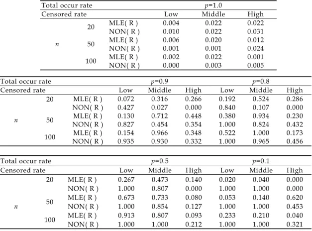
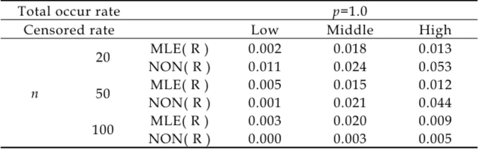
2.模擬結果

從

Table 1 及 Table 2 來看可以知道在

確定母體分布後，

MLE(R)之方法其顯著水

準之維持相當小，尤其在低設限率時，很容

易接受虛無假設。最主要原因是由於模式中

的參數都把訊息帶走，所以估到的

p 之值都

很接近

1，因此其檢定力表現相當的差，尤

其當在很高的『長期存活比例』時，也是因

為參數都把訊息吸收了，例如指數分布其平

均數都會高估，所以

p 值亦高估了。整體來

看，無母數方法較穩健。

Table 1. Results of MLE(R) and NON(R) when distribution of T is exponential.

Total occur rate p=1.0

Censored rate Low Middle High

MLE( R ) 0.004 0.022 0.022 20 NON( R ) 0.010 0.022 0.031 MLE( R ) 0.006 0.020 0.012 50 NON( R ) 0.001 0.001 0.024 MLE( R ) 0.002 0.022 0.001 n 100 NON( R ) 0.000 0.003 0.005

Total occur rate p=0.9 p=0.8

Censored rate Low Middle High Low Middle High

MLE( R ) 0.072 0.316 0.266 0.192 0.524 0.286 20 NON( R ) 0.427 0.027 0.000 0.840 0.107 0.000 MLE( R ) 0.130 0.712 0.448 0.380 0.934 0.230 50 _NON(_R_{) 0.827 0.454 0.354 1.000 0.824 0.432} MLE( R ) 0.154 0.966 0.348 0.522 1.000 0.173 n 100 _NON(_R_{) 0.935 0.930 0.332 1.000 0.965 0.456}

MLE( R ) 0.267 0.473 0.140 0.020 0.040 0.000 20 NON( R ) 1.000 0.807 0.000 1.000 1.000 0.000 MLE( R ) 0.673 0.733 0.080 0.053 0.140 0.620 50 NON( R ) 1.000 0.854 0.127 1.000 1.000 0.453 MLE( R ) 0.913 0.807 0.093 0.233 0.210 0.040 n 100 NON( R ) 1.000 1.000 0.212 1.000 1.000 0.321

(9)

Table 2. Results of MLE (R) and NON (R) when distribution of T is Weibull.

Total occur rate p=1.0

Censored rate Low Middle High

MLE( R ) 0.002 0.018 0.013 20 NON( R ) 0.011 0.024 0.053 MLE( R ) 0.005 0.015 0.012 50 NON( R ) 0.001 0.021 0.044 MLE( R ) 0.003 0.020 0.009 n 100 NON( R ) 0.000 0.003 0.005

MLE( R ) 0.182 0.333 0.221 0.188 0.524 0.286 20 NON( R ) 0.389 0.033 0.001 0.620 0.112 0.001 MLE( R ) 0.130 0.712 0,448 0.380 0.934 0.230 50 NON( R ) 0.827 0.454 0.354 0.982 0.824 0.432 MLE( R ) 0.154 0.894 0.348 0.526 0.909 0.168 n 100 NON( R ) 0.735 0.850 0.332 1.000 0.965 0.511

MLE( R ) 0.146 0.393 0.132 0.020 0.040 0.000 20 NON( R ) 0.933 0.947 0.001 1.000 1.000 0.000 MLE( R ) 0.673 0.733 0.077 0.053 0.139 0.620 50 NON( R ) 1.000 0.854 0.118 1.000 1.000 0.453 MLE( R ) 0.913 0.801 0.090 0.233 0.210 0.040 n 100 NON( R ) 1.000 1.000 0.233 1.000 1.000 0.122

結論

在種子發芽行為模式之建立，從過去的

文獻探討上，已經有許多的學者提出其不同

之見解。本文將此種發芽行為資料，利用其

觀察等待發芽成功的時間，解釋成為存活時

間，對於未能在觀察時間內發芽之種子資

料，視為一種設限資料。但是種子在發芽的

行為中，會受到溫度之影響，有可能在長期

的實驗之下，種子永遠不會發芽。因此我們

將此種種子的資料視為右方設限長期存活

資料，引進存活分析統計方法，來建立種子

長期存活資料的發芽比率之統計推論。

在右方設限資料中，若資料中有「長期

存活資料」時，我們建議可採用最大概度估

計法或無母數方法來估計「長期存活資料」

之比例，當然在不同的資料型態下，必須引

用不同的方法。然而最大概度估計法會受限

到母體之分布情形，因此在引用之前必須經

由適合度檢定，若不滿足假設母體之定義，

採用無母數方法應是較為保守之作法。

引用文獻

Allison PD (1995) Survival Analysis Using the SAS System: A Practical Guide. p.29-60, p.61-87. SAS Institute Inc., NC, USA.

Bahler C, RR Hill, RA Byers (1989) Comparison of logistic and Weibull functions: the effect of temperature on cumulative germination of

(10)

alfalfa. Crop Sci. 29:142-146.

Boag JW (1949) Maximum likelihood estimates of the proportion of patients cured by cancer therapy. J. Royal Statist. Soc., Series B 11:15-44.

Brown RF (1987) Germination of Aristida armata under constant and alternating temperatures and its analysis with the cumulative Weibull distribution as a model. Aust. J. Bot. 35:581-591.

Janssen JGM (1973) A method of recording germination curves. Ann. Bot. 37:705-708. Dumur D, CJ Pilbeam, J Craigon (1990) Use of the

Weibull function to calculate cardinal temperatures in faba bean. J. Exp. Bot. 41:1423-1430.

Farewell VT (1977) A model for a binary variable with time censored observations. Biometrika 64:43-46.

Farewell VT (1982) The use of mixture models for the analysis of survival data with long-term survivors. Biometrics 38:1041-1046.

Goldman AI (1984) Survivorship analysis when curve is a possibility: a Monte Carlo study. Statist. Medicine 3:153-163.

Gordon NH (1990) Application of the theory of finite mixtures for the estimation of ‘cure’ rates

of treated cancer patients. Statist. Medicine 9:397-407.

Haybittle L (1965) A two–parameter model for the survival curve of treated cancer patients. J. Amer. Statist. Assoc. 60:16-26.

Huang CH, CM Yang (1995). Use of Weibull function to quantify temperature effect on soybean germination. Chinese Agron. J. 5:25-34.

Su HY, CH Su, HL Wang (2000) Survival analysis of the effect of temperature on germination of seeds. Chinese Agron. J. 10:71-82.

Su HY, IC Huang, HN Hsieh (2003) The interval censored survival analysis for the effect of temperature on germination of seeds. Chinese Agron. J. 13:141-149.

Kaplan EL, P Meier (1958) Nonparametric estimation from incomplete observations. J. Amer. Statist. Assoc. 53:457-481.

Maller RA, S Zhou (1992) Estimating the proportion of immunes in a censored sample. Biometrika 79:731-739.

Maller RA, S Zhou (1996) Survival Analysis with Long-time Survivors. p.67-79, p.97-104. Wiley, New York.

Thornley JHM (1977) Germination of seeds and spores. Ann. Bot. 41:1363-1365.

右方設限長期存活資料比率之研究