* Corresponding author. Tel.: #886-2-2366-1931; fax: #886-2-2362-2975. E-mail address: hkhong@ce.ntu.edu.tw (H.-K. Hong)
Internal symmetry in the constitutive model
of perfect elastoplasticity
Hong-Ki Hong*, Chein-Shan Liu
Department of Civil Engineering, National Taiwan University, Taipei 106-17, Taiwan
Received 8 February 1999; accepted 29 March 1999
Abstract
Internal symmetry in the constitutive model of perfect elastoplasticity is investigated here. Using homogeneous coordinates, we convert the non-linear model to a linear system XQ "AX. In this way the inherent symmetry in the constitutive model of perfect elastoplasticity (in the on phase) is brought out. The underlying structure is found to be the cone of Minkowski spacetimeMn`1 on which the proper orthochronous Lorentz group SO0(n,1) left acts. When the plasticity mechanism is shut o! by the input path, the internal symmetry is switched to a translation group ¹(n) acting on the closed discDn of Euclidean space En. Based on the group properties a Cayley transformation is developed, which updates the stress points to be automatically on the yield surface at every time increment. These results (and their generalizations to more sophisticated models) are essential for computational plasticity. As an example, the results calculated using the group-preserving scheme and the exact constitutive solutions for a rectilinear path are com-pared. ( 1999 Elsevier Science Ltd. All rights reserved.
Keywords: Perfect elastoplasticity; Internal symmetry; Minkowski spacetime; Lorentz group; Group-preserving scheme
1. Introduction
The study of plastic behavior of solid materials and structural members under complicated mechanical environment is a very important topic for engineering science and industrial practice. In the study a substan-tial role has been played by the constitutive relations of elastoplasticity, to which many theoretical and experimental contributions have been made. However, it seems to authors' knowledge that there was no attempt in open literature until recently to study symmetry groups in the constitutive models of plasticity.
A constitutive model of plasticity is said to possess internal symmetry if it retains the forms of expressions for certain plastic phenomena even after changes in the states of the model have occurred. The changes or transformations occurring in the states of the model which leave the forms unchanged may constitute a Lie
0020-7462/99/$ - see front matter ( 1999 Elsevier Science Ltd. All rights reserved. PII: S 0 0 2 0 - 7 4 6 2 ( 9 9 ) 0 0 0 3 0 - X
Nomenclature
q, q%, q1 generalized strain, generalized elastic strain and generalized plastic strain
k%, Q0 generalized elastic modulus and generalized yield stress Q generalized stress
q0 equivalent generalized plastic strain
q: generalized yield strain
En, Dn, Bn, Sn~1 Euclidean n-space, closed n-disc, closed n-ball and n-sphere Mn`1, g Minkowski spacetime and Minkowski metric
X, X0, X4 augmented stress, temporal coordinate and spatial coordinates ¹
(n), SO0(n, 1) translation group and proper orthochronous Lorentz group so(n, 1) Lie algebra of proper orthochronous Lorentz group
A control tensor
W, SO(3) three-dimensional spin tensor and three-dimensional proper rotation group dX, dQ Minkowskian length of dX and Euclidean length of dQ
I0/ on interval of plasticity
t0, ti, t1, t zero-value time, initial time, time and current time i, *t a parameter and time increment
G, Cay(iA) Lorentz transformation tensor and Cayley transformation
group of transformations and are naturally linked with the invariance of certain conserved quantities. A procedure for parameter estimation (and model identi"cation) with e!ective utilization of the invariance properties along the experimental path will be more capable of capturing key features during plastic deformation. The passage from a #ow plasticity model to a computational plasticity scheme inhibits a symmetry group analysis since the scheme does not usually have the same group properties as the #ow model. A numerical algorithm which preserves symmetry in time marching will have long-term stability and much higher e$ciency and accuracy.
In fact, the most important invariance of a model of plasticity is that the changing stress states remain on the (subsequent) yield surface during plastic deformation. That is the so-called consistency condition. Once one "nds internal symmetry in a model of plasticity, he ensures among others the ful"llment of the consistency condition.
In this paper we propose to approach the symmetry issue and the computational application at the simplest three-dimensional model * perfect elastoplasticity. Generalizations to more sophisticated models will be hinted in due course (Section 11). We analyze the constitutive model of perfect elastoplasticity and attempt to achieve a deeper understanding of its underlying structure; more precisely speaking, we explore the structure of Minkowski spacetimeMn`1 and the proper orthochronous Lorentz group SO0(n,1) inherent in the model in the on phase and also address the symmetry switching between the on (i.e. elastoplastic) and o! (i.e. elastic) phases. To this end we need an appropriate setting to make the presentation clearer yet simpler, and, therefore, choose here to formulate the constitutive model directly in vector form. Let us consider the following constitutive model:
q5 "q5%#q51, (1)
QQ "k%q5%, (2)
1 The notation and terminology were used by Prager [1,2] and many other scholars.
2 Model (1)}(6) describes only the deviatoric part of the Prandtl}Reuss behavior under small deformation. The volumetric part of the Prandtl}Reuss behavior is linearly elastic and is thus excluded from the present study in order to focus on the more interesting elastic}plastic behavior of the deviatoric part.
EQE)Q0, (4)
q5 0*0, (5)
EQEq50"Q0q50. (6)
Here Q and q5 are a pair of dual vectors in n-dimensional Euclidean space En; Q"col(Q1, Q2,2, Qn)" col(Q1,Q2,2, Qn) denotes the generalized stress vector and q5"col(q51, q52,2, q5n)"col(q51,q52,2, q5n) denotes the generalized strain rate vector.1 The above constitutive model is re-postulated from the celebrated Prandtl}Reuss equation formulated by Prandtl [3] and Reuss [4], which is well known as the simplest (yet rather useful) three-dimensional constitutive law for describing a class of linearly elastic-perfectly plastic materials. Further explanations of the notation and the model are delegated to the next section.
The vector space of Q is an ordinary Euclidean space, which is endowed with a positive dexnite inner product. Later on, in Section 4, an augmented vector space will be built and endowed with an indexnite inner product. Although plasticity models are known to be highly nonlinear, the perfect elastoplasticity model (1)}(6) will be analyzed in Section 3 and synthesized and converted in Section 5 into a two-phase linear system with an on-o! switch, and will be further examined in Section 6 concerning its Minkowski space-time structure. Owing to the implicit linearity, a Lorentz group of transformations for the augmented vectors is discovered in Section 7. A projective transformation for the generalized stress responses is then realized in Section 8. Sections 9 and 10 address computation, one for rectilinear paths and the other for general paths.
2. Perfect elastoplasticity
The generalized stress vector Q may coincide with the stress deviator at a material point (and its neighborhood in the external space) as in the Prandtl}Reuss case,2 or it may stand for the vector of stress resultants on a cross section of a structural member like a beam, column, beam}column connection, plate, shell, or machine part, etc., or it may be the restoring forces integrated at the nodes of "nite elements of a discretized continuum. The generalized strain vector q and the generalized strain rate vector q5 are assumed to be so small that no account is taken of the spinning e!ect and the rate e!ect as well as the inertia e!ect.
As usual, the norm of a vector, say Q, in Euclidean spaceEn is de"ned asEQE:"JQ5Q where Q5Q denotes the Euclidean inner product+ni/1QiQi and the superscript t represents the transpose. The generalized elastic modulus k%'0 and the generalized yield stress Q0'0 are the only two characteristic constants of the model, which are determined experimentally. The boldfaced symbols q% and q1 are the n-dimensional (Euclidean) (column) vectors of generalized elastic and plastic strains, respectively, whereas q0 is a scalar called the equivalent generalized plastic strain, with Q0q50 being the (speci"c) power of dissipation. All q,q%,q1, Q and
q0 are functions of one and the same independent variable, which in most cases is taken either as the ordinary
time or as the arc length of an input path; however, for convenience, the independent variable no matter what it is will be simply called (the external) time and given the symbol t. An overdot denotes di!erentiation with respect to time, that is d/dt. Without loss of generality it is also postulated that with the above di!erential
model there is a time instant designated as t"t0, called the zero-value (or annealed) time, before and at which the model is in the zero-value (or annealed) state in the sense that the relevant values q(t0),q%(t0), q1(t0), Q(t0) and q0(t0) are all zeros.
Eq. (1) decomposes the generalized strain rate into the elastic and plastic parts, and Eq. (2) states a linear relation for the elastic part whereas Eq. (3) is an associated plastic-#ow rule for the plastic part. Inequality (4) speci"es admissible generalized stresses; we often callEQE)Q0 the admissible closed ball, EQE'Q0 the forbidden exterior, andEQE"Q0 the yield hypersphere. Inequality (5) or Q0q50*0 requires the (speci"c) power of dissipation be nonnegative. It is easy to comprehend and appreciate Eqs. (1)}(5); however, Eq. (6) may need more explanation. With the aid of Eqs. (4) and (5), it simply requires q0 be frozen if EQE(Q0, so that q5 0"0 drastically reduces Eqs. (1)}(3) to QQ"k%q5, a linearly elastic relation. The signi"cance of the complementary trios (4)}(6) cannot be overemphasized. It furnishes the model with an on}o! switch for the mechanism of plasticity, and the conditions to switch on and to switch o! the mechanism can thus be derived in a very precise way. Therefore, depending upon the input path, the model can be either in the ON (or elastoplastic) phase governed by Eqs. (1)}(3) or in the OFF (or elastic) phase governed by QQ "k%q5, as will be made clear in the next section.
3. Switch for the mechanism of plasticity
In this section we analyze #ow model (1)}(6), deriving the on}o! switching criteria for the mechanism of plasticity [5].
In the study of rate-independent plasticity we are always concerned with paths. By a path we mean a continuous curve whose velocity vectors are piecewise continuous. From Eqs. (3), (5) and (6) and Q0'0, it is not di$cult to prove that
q5 0"Eq51E, (7)
that is, q0 is the arc length of a path in the generalized plastic strain space. Substituting Eqs. (2) and (3) into Eq. (1) gives
1 k%QQ # q5 0 Q0Q"q5 (8) or d dt(X0Q)"k%X0q5, (9)
where the integrating factor
X0 :"exp
A
q0q:
B
(10)is called the internal time, in which the generalized yield strain is de"ned as
q: :"Qk%0. (11)
Taking the Euclidean inner product of Eq. (8) with Q gives 1
k%Q5QQ# q5 0
which, due to the constancy of Q0, asserts
EQE"Q0NQ5q5"Q0q50, (13)
or in terms of X0 via Eq. (10), EQE"Q0NXQ 0 X0" Q5 Q0 q5 q:. (14)
Since Q0'0, we have by Eq. (13)
EQE"Q0NMQ5q5'0Qq50'0N. (15)
Thus we have deduced the `Na part of the following statement:
MEQE"Q0 and Q5q5'0NQq50'0. (16)
On the other hand, if q5 0'0, Eq. (6) ensures EQE"Q0, which together with Eq. (15) proves the `=a part of the above statement. In other words, the yield conditionEQE"Q0 and the straining condition Q5q5'0 are su$cient and necessary for plastic irreversibility q5 0'0. Considering Eq. (16) together with Eqs. (4), (5), (7) and (13), we obtain the following on}o! switching criteria for the mechanism of plasticity:
q5 0"Eq51E"
G
1
Q0Q5q5'0 if EQE"Q0 and Q5q5'0,
0 ifEQE(Q0 or Q5q5)0.
(17)
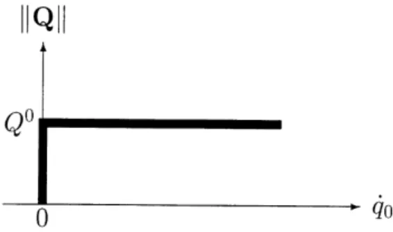
Based on the criteria and the complementary trios (4)}(6), there are precisely two phases: the ON phase in which q5 0'0 and EQE"Q0 and the OFF phase in which q50"0 and EQE)Q0; see Fig. 1. In the on phase the mechanism of plasticity is on and the model exhibits elastoplastic behavior, which is irreversible, while in the o! phase the mechanism of plasticity is o! and the model responds elastically and reversibly.
4. Minkowski spacetime Let us de"ne X"
C
X4 X0D
"C
X1 X2 F Xn X0D
:"exp(q0/q:) Q0C
Q Q0D
"exp(q0/q:)Q0C
Q1 Q2 F Qn Q0D
(18)and call it the (n#1)-dimensional augmented stress vector. Note that the last component of Eq. (18) is consistent with Eq. (10) and that the components of the generalized stress vector Q and the components of the augmented stress vector X are indeed the non-homogeneous and homogeneous coordinates of the same stress state. Two augmented stress vectors which only di!er by a non-zero scalar multiple represent the same generalized stress vector.
Now we recast model (1)}(6) postulated in the generalized stress space of Q into a model in the augmented stress space of X. Accordingly, Eqs. (9), (6), (4), and (5) become
Fig. 1. The complementary trios (4)}(6) specify the admissible region in the phase plane of (q5 0,EQE), which is marked by heavy lines.
3 Following [6] we refer the null cone emanating from X"0 as the cone. 4 The time-like region of X"0.
5 The space-like region of X"0.
C
In 0nC1 01Cn X5gXD
XQ " 1 q:C
0nCn q5 01Cn 0D
X, (19) X5gX)0, (20) XQ 0*0, (21)in terms of the Minkowski metric (in the space-like convention) g"
C
g44 g40g04 g00
D
"
C
In 0nC1 01Cn !1D
, (22)
where In is the identity tensor of order n. The vector space of augmented stresses X endowed with the Minkowski metric tensor g is referred to as Minkowski spacetime and designated asMn`1.
Spacetime of this sort underlying the constitutive theory may be called internal spacetime, because we can think of it as having to do with the intrinsic nature of the mechanical behavior of the solid materials or the structural members which the constitutive model describes, rather than their position or motion in ordinary (external) space and (external) time. Thus the `temporala coordinate X0 and the `spatiala coordinates X4"(X1, X2,2, Xn) may be thought of as the internal time and the internal space, respectively. In this treatment X0 and X4 are no more disparate and incompatible as the usual (n#1)-dimensional vector in Euclidean spacetimeEn`1; they are now being organized to an integrated object in Minkowski spacetime Mn`1, which is not a simple extension of ordinary Euclidean n-space to n#1 dimensions, with X0 as just one more dimension. Because the corresponding entries in the metric have di!erent signs, !1 versus positive de"niteness, the `temporala coordinate X0 is not on the same footing as the n `spatiala coordinates (X1, X2,2, Xn), and the structure built on the spacetime consequently has group properties (see Sections 7 and 8) quite unlike that on Euclidean space.
Regarding Eqs. (4) and (20), we may further distinguish two correspondences:
EQE"Q0QX5gX"0, (23)
EQE(Q0QX5gX(0. (24)
That is, a generalized stress vector Q on (resp. within) the yield hypersphereEQE"Q0 in the generalized stress space of (Q1, Q2,2, Qn) corresponds to an augmented stress vector X on the cone3 MXDX5gX"0N of Minkowski spacetime (resp. in the interior4 MXDX5gX(0N of the cone). The exterior5 MXDX5gX'0N of the
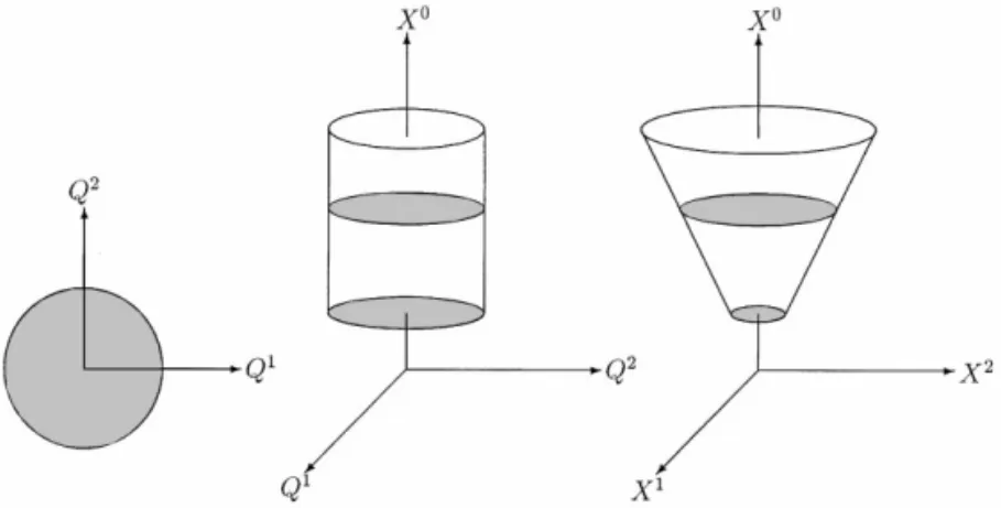
Fig. 2. The conventional concept of yield hypersphereSn~1 in the generalized stress space Q may be extended to a cylinder in the product space of (Q, X0); however, it is the construction of the cone in Minkowski spacetime of X that signi"esa conceptual breakthrough. A few discs of simultaneity are also shown.
cone is uninhabitable sinceEQE'Q0 is forbidden according to axiom (4). Even though it admits an in"nite number of Riemannian metrics, the yield hypersphereSn~1 in the Q-space does not admit a Minkowskian metric, nor does the cylinder in the (Q5, X0)-space. It is the cone in the X-space which admits the Minkowski metric. As an illustration, a schematic plot is shown in Fig. 2.
Taking the Euclidean inner product of Eq. (9) with Q and substituting Eq. (18), we have 1 Q0q:Q5q5" 1 (X0)2 d dt[(X4)5g44X4].
Upon considering Q0'0, q:'0 and X0*1, we have Q5q5'0 Qd
dt[(X4)5g44X4]'0, (25)
Q5q5)0 Qd
dt[(X4)5g44X4])0. (26)
Hence in the augmented stress space what corresponds to the yield conditionEQE"Q0 is the cone condition X5gX"0 and what corresponds to the straining condition Q5q5'0 is the growing `spatiala radial coordinate condition d[(X4)5g44X4]/dt'0.
In view of Eqs. (18) and (23)}(26), the on}o! switching criteria (17) become
XQ 0"(X4)5(q5/q:)'0 if X5gX"0 and (d/dt)[(X4)5g44X4]'0, (27a)
XQ 0"0 if X5gX(0 or (d/dt)[(X4)5g44X4])0, (27b) in the augmented stress space.
5. Two-phase systems
In this section, using the on}o! switching criteria, we synthesize and convert #ow model (1)}(6) to two-phase systems, searching for as revealing representations as possible. The following are three representa-tions, respectively, in the Q-spaces, the (Q, X0)-space, and the X-space. The three spaces have been illustrated in Fig. 2.
5.1. Non-linear representation in the Q-space
Using Eq. (17) to eliminate q0 from Eq. (8) results in a two-phase non-linear system of n equations: QQ "
G
!(Q5/Q0)(q5/q:)Q#k%q5 if EQE"Q0 and Q5q5'0,
k%q5 if EQE(Q0 or Q5q5)0, (28)
of which the latter is linear and represents an instantaneous response, and the former is a system of non-linear di!erential equations. This is a non-non-linear representation in the n-dimensional space of Q"(Q1, Q2,2, Qn).
5.2. Representation in the (Q, X0)-space
In the (Q, q0)-space, or equivalently in the (Q, X0)-space, the two-phase system of n#1 Eqs. (8) and (17), is non-linear. However, we may arrange the solution process in two steps, making the problem `lineara in a certain sense.
The solution of Eq. (9) is Q(t)"X0(ti) X0(t)Q(ti)#k%
P
t ti X0(m) X0(t)q5 (m) dm. (29)Substituting this into Eq. (17), using Eqs. (10) and (11) to change q0 to X0, integrating, and changing the order of the double integral, we "nally obtain [7]
X0(t)"
G
M1#(1/q:Q0)[q(t)!q(ti)]5Q(ti)NX0(ti)#(1/q2:):tti[q(t)!q(m)]tq5(m)X0(m) dm if EQE"Q0 and Q5q5'0,
X0(ti) if EQE(Q0 or Q5q5)0.
(30)
The "rst of Eq. (30) is a linear Volterra integral equation. Thus, given the q-path, we "rst solve Eq. (30) for
X0(t) and then calculate Q(t) via Eq. (29). 5.3. Linear representation in the X-space
Organizing Eqs. (9), (27a) and (27b) with the aid of Eq. (18), we have the augmented stress (linear di!erential) equation
XQ "AX (31)
with the control tensor
A :"1/q:
C
0nCnq5 5 q05D
if X5gX"0 and (d/dt)[(X4)5g44X4]'0, (32a) A :"1/q:C
0nCn01Cn q05D
if X5gX(0 or (d/dt)[(X4)5g44X4])0. (32b) It is remarkable that in the augmented stress space the two-phase system becomes linear. All together it is a two-phase linear system with an on}o! switch. The control tensor A in the on phase possesses the following properties: A5"A, tr A"0, det A"0, and its eigenvalues are 0 of multiplicity n!1 and $Eq5E/q:. As usual,the superscript t stands for the transpose, the symbol tr for the trace, and det for the determinant. The last row of the o!-phase's A is full of zeros since X0 is constant (i.e., q0 is "xed) in the o! phase. Thus we have revealed the linearity of the perfect elastoplasticity model both in the on and o! phases.
5.4. Comments
The multi-phase non-linear problems of plasticity were usually treated by workers in plasticity with various numerical schemes, which often encounter the tremendous di$culties of plastic non-linearity and yield inconsistency. The passage directly from #ow model (1)}(6) to a numerical scheme, if no care is taken of, may alter or destroy the underlying structure of the model, resulting in unstable, ine$cient, and inaccurate calculations. The passage from the above three representations to numerical schemes has the merit of the automatic ful"llment of the consistency condition. However, a numerical scheme based on the representation (28) in the Q-space su!ers from non-linearity. A numerical scheme based on the representation in the (Q, X0)-space, being non-linear but essentially `lineara in the above sense, has been shown to be much more e$cient [8].
Comparing the two representations (28) and (31), we observe that Eq. (28) is non-linear and of the n order, but Eq. (31) is linear and of the n#1 order; hence, the implicit linearity is unfolded at the expense of raising one order up. The representation in the X-space is linear, as just said, and, moreover, easy to retain the internal symmetries of the model, thus facilitating the ful"llment of the consistency condition. Therefore, we will focus on the linear representation in the X-space in the remainder of the paper.
6. Properties of paths in Minkowski spacetime
The augmentation of the states in n dimensions to n#1 dimensions is far more than a mere mathematical arti"ce. In this section the rich properties of the paths admissible in Minkowski spacetime will be explored. Criteria (17) ensure that
q5 0Q5QQ"0, (33)
no matter whether in the on or in the o! phase. In view of Eqs. (3), (7) and (5) and of the positivity of the two characteristic constants, Eqs. (8) and (33) become, respectively,
1
k%QQ #q51"q5, (34)
(q5 1)5QQ"0, (35)
which together indicate a right-angled triangle; therefore, according to the Pythagorean theorem,
0)q5 0"Eq51E)Eq5E, (36)
dQ :"EdQE"k%JEdqE2!(dq0)2, (37)
(q5 1)5q5*0, (38)
all of which are valid for both the on and o! phases, even though the triangle may degenerate to a line segment or even to a single point. What do these important observations (36)}(38) imply for a path in the Minkowski spacetime of augmented stresses?
6.1. Time-like paths are not allowed
We "rst examine Eq. (36), which tells us that the minimum and maximum values of the (speci"c) dissipation power"Q(t)"Q0q50(t) an admissible path in the generalized stress space may discharge are zero and Q0Eq5(t)E, respectively. From Eqs. (36), (5), (10) and (11), it follows that
(X0)2q55q5!q2:(XQ0)2*0. (39)
Substituting Eqs. (9), (18) and (22) into the above equation, we obtain
XQ 5gXQ*0. (40)
Thus
(dX)2 :"dX5g dX*0. (41)
Be cautious not to mix up dX with dX0. The former is the Minkowskian length of the path increment dX, while the latter is the`temporala component of dX. Recalling that a path such that dX5g dX'0 (resp."0, (0) is called a space-like (resp. null, time-like) path in Mn`1, we thereby conclude that the curve X(t@),
ti(t@)t, in the augmented stress space is a space-like or null path in the Minkowski spacetime Mn`1 no
matter in the on or in the o! phase. Here ti denotes an initial time and t the current time. Indeed, Eq. (41) conveys an extremely important message that the nature of (perfect) elastoplasticity rejects time-like paths. As such the time-like metric convention has to be rejected to avoid an unreasonable negative squared length; this is the reason why we have adopted the space-like convention (22) for plasticity.
6.2. Space-like paths versus null paths
Regarding Eqs. (36) and (41), we may further distinguish q5 0(Eq5E from q50"Eq5E and identify the former with the space-like path and the latter with the null path, as in the following two categories:
q5 0(Eq5E Q q51Oq5 Q QQO0 Q a regular Q-path
Q XQ5gXQ'0 Q X0XQOXQ0X Q dX'0 Q a space-like X-path versus
q5 0"Eq5E Q q51"q5 Q QQ"0 Q a "xed Q-point
Q XQ5gXQ"0 Q X0XQ"XQ0X Q dX"0 Q a null X-path. (42) A regular path refers to a path whose velocity vectors do not vanish. Most of practical situations fall into the "rst category of Eq. (42) * a regular path in the vector space of generalized stresses, or, correspondingly, a space-like path in the augmented stress space * in which the maximum in Eq. (36) is further sharpened to be a supremum. A few remarks on the second category of Eq. (42) are in order. In the vector space of generalized stresses the second category is a "xed point, which appears to be the projection of a null path, i.e. a ray on the null cone emanating from the origin X"0 of the augmented stress space. If QQ "0, then from Eq. (28) either q5 "0, which is trivial since nothing happens, or q5" constant (namely, the generalized strain path is rectilinear) and
Q"QM :"Q0q5/Eq5E
(namely, the generalized stress path stops and remains "xed at the point QM , which may be interpreted as a limit strength vector), in which q5 "constant. The super"cial impression that the generalized stress}strain curve of perfect elastoplasticity is merely an inclined straight line followed by a horizontal line in fact stems
from the second category. All the one-dimensional cases (n"1) fall into the second category, but for the dimensionality n*2 the situations which fall into the second category are relatively rare [7]. The distinctive behavior for n"1 is rooted in topology: its yield hypersurfaceEQE"Q0 in the vector space of generalized stresses is disconnected and contains only two points, so that in the on phase Q has no room to move unless to switch o!.
6.3. Relation between the Euclidean and Minkowskian lengths
Next, we study Eq. (37), which, in view of Eqs. (9)}(11), (18), (22) and (41), amounts to dX
X0"
dQ
Q0, (43)
no matter in the on or in the o! phase. In other words, the Minkowskian length dX of a di!erential element of a path in the augmented stress spaceMn`1 of (X1, X2,2, Xn, X0) is X0/Q0 times the Euclidean length dQ of the corresponding di!erential element of the corresponding path in the generalized stress space En of (Q1, Q2,2, Qn).
6.4. Nguyen}Bui inequality
Finally we study inequality (38). Constitutive models which satisfy Eq. (38) are said to be kinematically stable [9]. By Eqs. (3) and (18) we have
q5 1"qyXQ0 (X0)2X4.
From Eqs. (31), (32a) and (32b) it follows that q5 "qy
X0XQ 4.
Both the above two equations are valid no matter whether in the on or in the o! phase. Thus Eq. (38) turns out to be
XQ 0d
dt[(X4)5g44X4]*0. (44)
In the derivations of the above three equations we have used q:'0 and X0*1. Inequality (44) just says again the fact that either the`temporala coordinate is "xed (i.e., X is on the closed disc for the o! phase) or the `spatiala radial coordinate of the X-path cannot be decreasing. This is rather transparent from the point of view of the geometry of the cone in the X-space. However, its equivalent version (38) in the Q-space is not trivial at all, its signi"cance having been pointed out in [9].
6.5. Paths on the cone
From Eqs. (13), (18) and (22) it follows that
EQE"Q0NX5g(q55, q50)5"0. (45)
Moreover, by Eqs. (27a), (31), (18) and (22) we can prove that
If the model is in the on phase (i.e., not onlyEQE"Q0 but also Q5q5'0), then from Eqs. (23), (45) and (46) it follows that for an X-path on the cone, the augmented stress vector X is M-orthogonal to itself, to its tangent vector XQ and also to its dual (q55, q50)5. The so-called M-orthogonality is an orthogonality of two (n#1)-dimensional vectors with respect to metric (22) in Minkowski spacetimeMn`1 (see, for example [10]).
It is worth comparing Eqs. (45) and (46) with Eqs. (20), (23), (24), (40) and (42).
6.6. Paths on the discs
On the other hand, X0 is frozen in the o! phase as indicated by Eq. (27b) and the augmented stressX stays in the closed n-disc Dn (i.e. closed n-ball Bn) on the hyperplane X0" constant in the space of (X1, X2,2, Xn, X0), the hyperplane being identi"ed to be Euclidean n-spaceEn, which is endowed with the Euclidean metric In. In summary, the augmented stress X either evolves on the cone when in the on phase or stays in the discs of simultaneity, which are stacked up one by one in the interior of the cone and are glued to the cone, when in the o! phase. See Fig. 2 again.
6.7. Future pointing non-time-like paths
The vector X(t)!X(ti) and the path MX(t@)Dti(t@)tN are said to be future-pointing if X0(t)'X0(ti) strictly. Therefore, the solution to Eq. (31) with Eq. (32a) can be viewed as a future-pointing space-like or null path on the coneMXDX5gX"0N, while the solution to Eq. (31) with Eq. (32b) is a space-like path on a closed disc of simultaneityMXDX5gX)0 and XQ0"0N. It is worth stressing that the interior of the cone is sliced into stacking discs of simultaneity tagged with di!erent values of X0; therefore, an admissible augmented stress can be reached either along paths in the discs of simultaneity when in the o! phase or along the future-pointing space-like or null paths on the cone when in the on phase.
7. The Lorentz group
In this section we concentrate on the on phase to bring out internal symmetry inherent in the model in the on phase. Denoted by I0/ an open, maximal, continuous time interval during which the mechanism of plasticity is on exclusively. The solution of the augmented stress equation (31) with Eq. (32a) can be expressed in the following augmented stress transition formula:
X(t)"[G(t)G~1(t1)]X(t1), ∀t,t13I0/, (47) in which G(t), known as the fundamental solution of Eq. (31), is a transformation tensor satisfying
GQ (t)"A(t)G(t), (48)
G(0)"In`1. (49)
On the other hand, from Eqs. (32a) and (22) it is easy to verify that the control tensor A in the on phase satis"es
A5g#gA"0. (50)
By Eqs. (50) and (48) we "nd d
6 From Eqs. (5), (10) and (18) it follows that X0(t)*X0(t@)*X0(ti)*X0(t0)"1 for all t*t@*ti*t0, applicable to both the on and o! phases. Recall that t0 is the zero-value time at which all relevant values including q0(t0)"0.
At t"0, G5(t)gG(t)"I5n`1gIn`1"g from Eq. (49); thus, we prove that
G5(t)gG(t)"g (51)
for all t3I0/. Take determinants of both sides of the above equation, getting
(det G)2"1, (52)
so that G is invertible. The 00th component of the tensorial equation (51) is+ni/1(Gi0)2!(G00)2"!1, from which
(G00)2*1. (53)
Here Gij, i,j"1,2,2,n,0, is the ijth mixed component of the tensor G. Since detG"!1 or G00)!1 would violate Eq. (49), it turns out that
det G"1, (54)
G00*1. (55)
In summary, G has the three characteristic properties explicitly expressed by Eqs. (51), (54) and (55). Recall that the complete homogeneous Lorentz group O(n, 1) is the group of all invertible linear transformations in Minkowski spacetime which leave the Minkowski metric invariant, and that the proper orthochronous Lorentz group SO0(n,1) is a subgroup of O(n,1) in which the transformations are proper (i.e., orientation preserving, namely the determinants of the transformations being #1) and orthochronous (i.e., time-orientation preserving, namely the 00th entry of the matrix representations of the transformations being positive); see, for example, [11]. Hence, in view of the three characteristic properties we conclude that the fundamental solution G belongs to the proper orthochronous Lorentz group SO0(n,1). Therefore, the tensor-valued function G(t) of time t3I0/ may be viewed as a connected path of the Lorentz group. Furthermore, by Eq. (50), A is an element of the real Lie algebra so(n, 1) of the Lorentz group SO0(n,1). Thereby the algebraic and topological properties of the proper orthochronous Lorentz group are shared by the perfect elastoplasticity model (1)}(6).
From Eq. (27a), XQ 0'0 strictly when the mechanism of plasticity is on; hence,6
X0(t)'X0(t1)'X0(t0)"1, ∀t't1't0, t,t13I0/, (56) which means that in the sense of irreversibility there exists future-pointing time-orientation from the augmented stress X(t1) to X(t). Moreover, such time-orientation is a causal one, because the augmented stress transition Eq. (47) and inequality (56) establish a causality relation between the two augmented stress vectors X(t1) and X(t) in the sense that the preceding augmented stress vector X(t1) in#uences the following augmented stress vector X(t) according to Eq. (47). Accordingly, the augmented stress vector X(t1) chrono-logically and causally precedes the augmented stress vector X(t). This is indeed a common property for all models with inherent symmetry of the proper orthochronous Lorentz group. By this symmetry a core connection among irreversibility, the time arrow of evolution, and causality has thus been established for plasticity in the on phase.
8. Projective realization
Relation (47) of the group of transformations can be made to be more useful especially when interpreted in terms of generalized stresses. To elaborate, we solve Eq. (51) for the inverse
G~1"gG5g (57)
and partition G as G"
C
G44 G40G04 G00
D
. (58)Thus, Eq. (47) is partitioned into
C
X0(t)Q(t)/Q0 X0(t)D
"C
G44(t)(G44)5(t1)!G40(t)(G40)5(t1) G40(t)G00(t1)!G44(t)G04(t1) G04(t)(G44)5(t1)!G00(t)(G40)5(t1) G00(t)G00(t1)!G04(t)G04(t1)DC
X0(t1)Q(t1)/Q0 X0(t1)D
. (59) Dividing the "rst row by the second row we haveQ(t)"M[G44(t)(G44)5(t1)!G40(t)(G40)5(t1)]Q(t1)Q0#[G40(t)G00(t1)!G44(t)G04(t1)](Q0)2N/
M[G04(t)(G44)5(t1)!G00(t)(G40)5(t1)]Q(t1)#[G00(t)G00(t1)!G04(t)G04(t1)]Q0N. (60) The transformation is known as a projective unimodular transformation, which maps Q(t1) to the current response Q(t). In fact the generalized stress Q, a vector with n components supposed to be observable, is a projective realization of the vector X which has n#1 homogeneous coordinates.
Contrary to Eq. (60) in the on phase, the mapping in the o! phase is very simple,
Q(t)"Q(t1)#k%[q(t)!q(t1)], (61)
where Q(t1) is the starting generalized stress vector at time t1 in the o! phase. It may be recast to the transformation of augmented stress vectors:
C
X0(t)Q(t)/Q0 X0(t)D
"G(t)G~1(t1)C
X0(t1)Q(t1)/Q0 X0(t1)D
(62) but with G(t)"C
In q(t)/q: 05 1D
. (63)Even such an o!-phase transformation of augmented stresses exists and is invertible; it is no longer an element of the Lorentz group because such G does not satisfy Eq. (51) although det G"1 remains to hold and G00"1. It belongs to a translation group ¹(n) on Bn of En. The change from a transformation of the Lorentz group in the on phase to a non-Lorentzian transformation in the o! phase indicates that internal symmetry switches from one kind to another.
9. Exact solutions for rectilinear paths
Consider a rectilinear generalized strain path q(t)"q(t1)#(t!t1)q5
with non-zero constant rate q5 "constantO0,
starting from q(t1) at time t1. The constitutive response can be determined exactly [7], and it may be recast in the form of Eq. (47) with the augmented stress transition tensor for the on phase being
G(t)G~1(t1)"
C
In#((a!1)/Eq5E2)q5q55 bq5 /Eq5Ebq5 5/Eq5E a
D
, (64)in which
a :"cosh[(t!t1)Eq5E/q:], b :"sinh[(t!t1)Eq5E/q:]. (65) To examine the group properties, we "nd the fundamental solution as
G(t)"
C
In#((a!1)/Eq5E2)q5q55 bq5 /Eq5Ebq5 5/Eq5E a
D
, (66)but with
a :"cosh(tEq5E/q:), b:"sinh(tEq5E/q:). (67)
It is not di$cult to see that the above G satis"es Eqs. (51), (54) and (55); therefore, the curve G(t) going through the identity G(0)"I at t"0 is a one-parameter subgroup of the Lorentz group SO0(n,1). The projective realization developed in Section 8 becomes for this case
Q(t)"Q0[Q(t1)#((a!1)/Eq5E2)q55Q(t1)q5]#b(Q0)2q5/Eq5E
bq5 5Q(t1)/Eq5E#aQ0 . (68)
This is the generalized stress response for the on phase, while in the o! phase it is replaced by Eq. (61). 10. Group preserving schemes for general paths
Now let us consider general paths of generalized strain inputs and "nd their responses. To devise numerical schemes for time marching, let us denote the time increment by*t and develop maps to update Q(t) to the next time step Q(t#*t).
10.1. A scheme for piecewise rectilinear paths
We may approximate a general path by a piecewise rectilinear path. Referring to Eq. (64), we obtain the desired map
G(t#*t)G~1(t)"
C
In#((a!1)/Eq5E2)q5q55 bq5 /Eq5Ebq5 5/Eq5E a
D
(69)with
a :"cosh(*tEq5E/q:), b :"sinh(*tEq5E/q:). (70)
Thus a numerical scheme for the on phase may be devised as follows: for each time increment "rst calculate the map (69), then update the augmented stress vector by
X(t#*t)"G(t#*t)G~1(t)X(t)
10.2. Cayley transform scheme for general paths
For A3so(n, 1) the group generated is known as a Lorentz rotation or boost group. For the Lorentz rotation, the Cayley transform
Cay(iA)"(I!iA)~1(I#iA) (71)
is also a map from A to an element of SO0(n, 1) for i3R and i2(q2:/Eq5E2. Substituting Eq. (32a) for A in the above equation yields
Cay(iA)"
C
In#2i2/(q2:!i2Eq5E2)q5q55 2iq:/(q2:!i2Eq5E2)q52iq:/(q2:!i2Eq5E2)q55 (q2:#i2Eq5E2)/(q2:!i2Eq5E2)
D
. (72) Thus we devise the Cayley transform scheme as follows: for each time increment "rst calculate the Cayley transform (72), then update the augmented stress vector byX(t#*t)"Cay(iA(t))X(t),
and "nally calculate the generalized stress vector Q(t#*t) via Eq. (18).
10.3. Comments on the two schemes
Comment 1. For the above two schemes, we must calculate X at each time step but need not calculate Q at every time step unless it is needed. We thus accelerate time marching and more e$ciently obtain the generalized stress response Q only at the target time instant.
Comment 2. Note that maps (69) and (72) satisfy the three characteristic properties (51), (54) and (55) of SO0(n,1); hence, the resultant schemes are both group preserving schemes. For the two schemes, the Lorentz group property ensures that, at every time step in the on phase, the maps update the augmented stress point to be always on the cone. As projective realizations, the generalized stress points in the on phase are, therefore, always located on the yield hypersphereSn~1, that is,
EQE"Q0 in the on phase.
This symmetry group property is essential for computational plasticity to completely avoid iterations, predictions and corrections, etc., in order to ful"ll the consistency condition.
Comment 3. A remarkable fact speci"c to a Lorentz rotation is that an exponential map of A admits a closed-form representation given by the following formula:
exp(*tA)"
C
In#((a!1)/Eq5E2)q5q55 bq5 /Eq5Ebq5 5/Eq5E a
D
(73)with a and b given by Eq. (70). Notice that exponential map (73) is just the G(t#*t)G~1(t) in Eq. (69). In terms of A given in Eq. (32a), the exponential map (73) for SO0(n, 1) acting on Mn`1 becomes
exp(*tA)"In`1#sinh
A
Eq5Eq:*t
B
q:AEq5E#C
coshA
Eq5E
q: *t
B
!1D
q2:A2Eq5E2. (74)
This is similar to the classical formula of Euler}Rodrigues for SO(3) acting onE3, exp(*tW)"I3#sin(w*t)W
w#[1!cos(w*t)]
W2
where W is a three-dimensional spin tensor and w is the Euclidean norm of the axial vector of W. Comment 4. If one takes
i"q:[1!cosh(*tEq5E/q:)]
Eq5Esinh(*tEq5E/q:) , (75)
the Cayley transform (72) is exactly equal to exponential map (73), that is,
Cay(iA)"exp(*tA). (76)
If one takes i"*t
2, (77)
the resulting is a time-centered Euler scheme. Therefore, the Cayley transform scheme accommodates more general input paths than piecewise rectilinear paths.
Comment 5. Similar to the above statement`Eq. (76) if Eq. (75)a for SO0(n,1) acting on Mn`1, a statement for SO(3) acting onE3 has been derived in [12] as follows:
Cay(iW)"exp(*tW) if i"2tan(w*t/2)
w*t . 10.4. Example
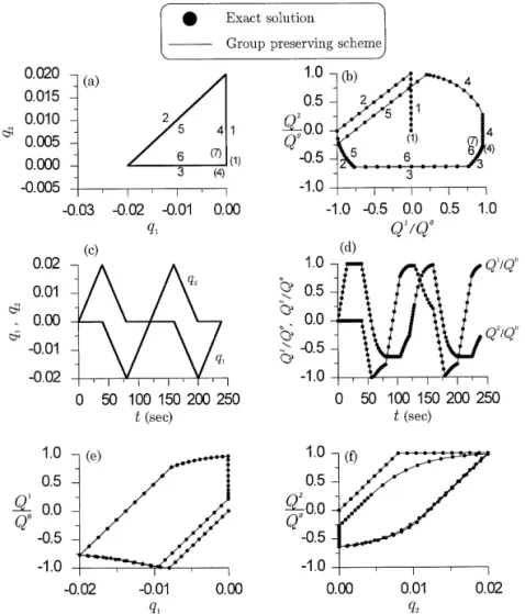
Fig. 3 displays an example of comparison between the exact solutions in Section 9 and the results calculated using the group preserving scheme in Section 10.1 for the model subjected to an input of a cyclic triangular path in two dimensions as shown in Fig. 3a. The "rst cycle consists of three pieces 1, 2, 3, the second cycle consisting of pieces 4, 5, 6 repeats in the generalized strain space the locus of the "rst cycle of pieces 1, 2 and 3, and so forth. The material constants used are k%"50000 MPa and Q0"400 MPa. Only the responses of the "rst two cycles are displayed because after those the responses were found to be almost repeated and stabilized. The results shown include the generalized stress path in Fig. 3b, hysteresis loops in Figs. 3e and f, time histories of generalized stresses in Fig. 3c. The response graph of the generalized stress path in Fig. 3b as can be seen is very di!erent from the input graph of the generalized strain path in Fig. 3a. One of two main features is that the generalized strain path is closed, but the corresponding generalized stress response has an open path. The points marked by (1), (4) and (7) in Fig. 3a are the same generalized strain points; however, the resulting generalized stress path 123 456 as shown in Fig. 3b starts at, passes through and ends at three di!erent generalized stress points marked by (1), (4) and (7), respectively. The other feature is that the generalized strain path is composed of straight lines, but the corresponding generalized stress response has straight-line paths in the o! phase but circular paths in the on phase. It is obvious that the group-preserving scheme gave very accurate responses and supplied a completely faithful result of the consistency condition.
11. Remarks on some generalizations
An element A of the real Lie algebra so(n, 1) which satis"es Eq. (50) has the general form A"
C
A44 A40Fig. 3. Comparison between the exact solutions and the results calculated using the group preserving scheme for the perfect elastoplastic model in two dimensions under a cyclic triangular generalized strain path: (a) input of the generalized strain path; (b) output of the generalized stress path; time histories of (c) generalized strains and (d) generalized stresses; hysteresis loops of (e) Q1 versus q1 and (f)
Q2 versus q2.
with the properties
(A44)5"!A44, A04"(A40)5.
But the earlier form of A as given in Eqs. (32a) and (32b) has zero A44 and is, therefore, less general than it may. We may generalize our model by including a non-vanishing, skew-symmetric tensor A44 if we no longer assume negligibly small spinning but instead consider large deformation and rotation [13].
A straightforward generalization of the Lorentz group SO0(n,1) is a PoincareH group, which is a semi-direct product of a translation group with the Lorentz group. In this way we can take the (linear [14] or non-linear) kinematic hardening}softening e!ect into consideration. In the on phase the augmented stress vectors remain on the cone. A generalization for this is to replace the cone by a hyperboloid, resulting in a model capable of accounting for the isotropic hardening}softening. A simultaneous generalization of the two thus renders mixed hardening.
Since the three generalizations brie#y mentioned above do not alter the core of the linear representation in the augmented stress space, the group preserving schemes for general paths presented in Section 10 and the exact solutions for rectilinear paths presented in Section 9 will be still applicable, after minor modi"cations and extensions, to the resulting more sophisticated models; in particular, the generalized stress point at every time step will be located automatically on the yield surface even when the yield surface moves kinematically and meanwhile expands (or contracts) isotropically. Note that the linearity in the augmented stress space and the automatic ful"llment of the consistency condition are essential for computational plasticity and both remain valid even after the suggested generalizations.
12. Conclusions
In this paper we have converted the constitutive model of perfect elastoplasticity to a two-phase system of linear di!erential equations in the (n#1)-dimensional augmented stress space of X. In the augmented stress space not only the non-linearity of the model was unfolded, but also an intrinsic spacetime structure of the Minkowskian type was brought out. The control tensor A which contains the generalized strain rate vector q5 was shown to be an element of the real Lie algebra so(n, 1) of the proper orthochronous Lorentz group SO0(n,1), and the fundamental solution G of the linear di!erential system (31) was proved to be an element of the Lorentz group, so that the causality relation of the augmented stresses was veri"ed. Based on the Lorentz group transformation (between X(t) and X(t1)) in the augmented stress space a projective transformation (between Q(t) and Q(t1)) in the generalized stress space was identi"ed such that the evolution rule of the generalized stress vectors became available. To account for both the on and o! phases a composite space endowed with a Minkowskian metric on the cone but with a Euclidean metric on each of the discs inside the cone may be constructed. As a result the perfect elastoplasticity model possesses two kinds of symmetry * ¹(n) (the translation group) in the o! phase and PSO
0(n, 1) (the projective realization of the proper orthochronous Lorentz group) in the on phase and has symmetry switching between the two depending on the generalized strain path input.
Using the symmetry group properties we have developed a Cayley transformation and devised the Cayley transform scheme, which possesses the crucial property that the generalized stress points are updated automatically on the yield surface at every time step. The scheme is applicable to general paths, while for rectilinear paths we have obtained exact solutions (68) and (61). These results (and their generalizations to the suggested more sophisticated models) are due to the symmetry group properties, among which the linearity in the augmented stress space and the automatic ful"llment of the consistency condition are particularly valuable for computational plasticity. An understanding of the internal symmetries in the underlying structure is not only important in its own right but also bene"cial to computation.
Acknowledgements
The "nancial support provided by the National Science Council under the Grant NSC 85-2211-E-002-001 is gratefully acknowledged. A preliminary version of the work presented here appeared as Chapter 2, pp. 7}29, of the report [15].
References
[1] W. Prager, The theory of plasticity: A survey of recent achievements, Proc. Inst. Mech. Engng 169 (1955) 41}57.
[3] L. Prandtl, Spannungsverteilung in plastischen kwrpern. In Proceedings of the 1st International Congress on Applied Mechanics, Delft, 1924, pp. 43}54.
[4] E. Reuss, Beruecksichtigung der elastischen formaenderungen in der plastizitaetstheorie, Zeits. angew. Math. Mech. (ZAMM) 10 (1930) 266}274.
[5] H.-K. Hong, C.-S. Liu, Prandtl}Reuss elastoplasticity: On-o! switch and superposition formulae, Int. J. Solids Struct. 34 (1997) 4281}4304.
[6] I.M. Gel'fand, M.I. Graev, N.Y. Vilenkin, Generalized Functions, Integral Geometry and Representation Theory, Vol. 5, Academic Press, New York, 1966.
[7] H.-K. Hong, C.-S. Liu, On behavior of perfect elastoplasticity under rectilinear paths, Int. J. Solids Struct. 35 (1998) 3539}3571. [8] H.-K. Hong, J.-K. Liou, Integral-equation representations of #ow elastoplasticity derived from rate-equation models, Acta Mech.
96 (1993) 181}202.
[9] Q.S. Nguyen, H.D. Bui, Sur les mateHriaux a` eHcrouissage positif ou neHgatif, J. de MeHcanique 13 (1974) 321}342. [10] G.L. Naber, The Geometry of Minkowski Spacetime, Springer, New York, 1992.
[11] J.F. Cornwell, Group Theory in Physics, Vol. 2, Academic Press, London, 1984.
[12] D. Lewis, J.C. Simo, Conserving algorithms for the dynamics of Hamiltonian systems on Lie groups, J. Non-linear Sci. 4 (1994) 253}299.
[13] H.-K. Hong, C.-S. Liu, Lorentz group SO
0(5, 1) for perfect elastoplasticity with large deformation and a consistency numerical scheme, Int. J. Non-Linear Mech. 34 (1999) 1113}1130.
[14] H.-K. Hong, C.-S. Liu, Internal symmetry in bilinear elastoplasticity, Int. J. Non-Linear Mech. 34 (1999) 279}288.
[15] H.-K. Hong, C.-S. Liu, Analyses, experimentation and identi"cation of dynamic system of elastoplasticity (2), Report prepared for the National Science Council Project No. NSC85-2211-E-002-001, Department of Civil Engineering, Taiwan University, Taipei, 1996.