1. Introduction
Entering the post genomic era, proteomic has become the topic that scientists are interested in. The authentication of protein has been an important item of the topics. For large datasets and fast tracks analysis, mass spectrometry has become an important tool for peptide analysis or proteomic authentication. On the clinical medical science, the most potential techniques of proteomic are mass spectrometry and protein chip. Mass spectrometry allows the determination of the molecular weight of peptides and proteins with a much greater accuracy than achievable by traditional methods. In addition, mass spectrometry experiments have become routine and can be performed within minutes.
Mass spectrometry (MS) is being used to discover diseased-related proteomic patterns in complex mixtures of proteins derived from tissue samples, or from biological fluids, such as serum, urine, or nipple aspirate fluid (Morris et al, 2005). We could diagnose disease early or find the reasons of the disease through these characteristics. This kind of technique has been widely used in biochip diagnosis or disease treatment. There are many applications about mass spectrometry such as oncology, ovarian cancer, and prostate cancer. Shiwa et al. (2003) found a potential biomarker for colon cancer from a mass spectrometry data set. They indicated that the ProteinChip System could perform the whole process of biomarker discovery from screening to evaluation of the identified marker. Petricoin et al. (2002) developed a bioinformatic tool and used it to identify proteomic patterns in serum that distinguish neoplastic from non-neoplastic disease within the ovary. Adam et al. (2002) built a high-throughput proteomic classification system. The system could be used to develop a highly accurate and innovative diagnostic advice for early detection of
prostate cancer. These results indicate that the mass spectrometry provide a powerful and valid tool in biomarker discovery of a certain disease. This high technology technique has been regarded as a new, efficient prophase-experimented method. If such technique could be spread out, it will be a great benefit to decrease the incidence rate and the mortality rate of a disease.
The categories of the mass spectrometry are MALDI-TOF MS (Matrix Assisted Laser Desorption/Ionization-Time of Flight Mass Spectrometry), SELDI-TOF MS (Surface Enhanced Laser Desorption/Ionization-Time of Flight Mass Spectrometry, ESI MS(Electro Spray Ionization Mass Spectrometry),etc. MALDI–TOF MS and SELDI-TOF MS are most commonly used mass spectrometry instruments in clinical and biological applications, see Morris et al. 2004. SELDI-TOF-MS can be considered as an extension of MALDI-TOF-MS method. In both cases, proteins to be analyzed are crystallized with UV-absorbing compounds and vaporized by a pulsed-UV laser beam. Ionized proteins are then accelerated in an electric field, and the mass to charge ratios of the different protein ion species can be deduced from their velocity. The differences between SELDI and MALDI are in the construction of the sample targets, the design of the analyzer and the software tools used to interpret the acquired data (Vorderwülbecke et al., 2005).
These potential clinical applications have made the development of better methods for processing and analyzing the data an active area of research. There are many related methods have been developed in literature. But mostly these methods are demonstrated through limited actual examples. Because of lack of theoretical derivations and numerical verifications, an objective evaluation to these methods is difficult.
results of a statistical method are derived under a hypothetical population distribution, a simulation can provide evidence to justify the results. Many data, for example, the spectra from a MS experiment, are complex by their very nature. For example, a spectrum from a MS experiment reveals not only important biological information of the sample but also is filled of uncertainties induced from the experiments. Theoretical results are hence difficult to obtain. In such circumstance, a simulation study plays an important role in assessing statistical methods. This study basically focuses on designing a simulation study of spectrum data from a virtual MS experiment.
Coombes et al. (2004) developed a virtual spectrometer of a simple MALDI-TOF experiment with time-lag focusing. The computation is based on a mathematical model, which takes the physical properties of the experiment into consideration. In their research, they explored several related characteristics of the virtual spectrometer. Subsequently, Morris et al. (2005) conducted a simulation study of mass spectrometry based on the virtual spectrometer to assess their proposed method. In our study, we follow the simulation procedure of Morris et al. (2005) and investigate more details about the virtual experiment.
The virtual experiment is divided into two stages: pre- and post-virtual spectrometer. The details will be fully described in the next two sections. In the beginning of the virtual experiment, a virtual population of the intensity of all possible proteins should be determined. A virtual sample is then randomly drawn from the population. In MS data, each detected peak indicates the relative intensity of a protein. However the intensity is generally different with the abundance-the number of molecules which have been ionized and desorbed from the biological sample-of that protein. Hence the virtual sample on intensity must be transferred to abundance based on an adequate calibration
model. The calibrated sample data are then put into the virtual spectrometer. Next section will illustrate the three components in the pre-virtual spectrometer stage: the determination of a virtual population, the generation of a virtual sample and the calibration process from intensity to abundance. The model in the calibration process is built according to some properties. These properties will be verified in this section.
In Section Three an introduction on the virtual mass spectrometer will be given firstly. When a biological sample enters the virtual spectrometer, the virtual spectrometer records the time of flight (TOF) of each ionized molecule in the biological sample. To obtain the mass-to-charge ratios (m/z) of proteins, a calibration procedure transferring TOF to m/z is necessary. The variability in the spectrometer and the calibration process result in location shift in m/z. The severity of error in m/z will be studied in this section. Some conclusions about the virtual experiment and suggestions for future research will be given in Section Four.
2 Pre-Virtual Spectrometer
A virtual mass spectrometry experiment is conducted by randomly generating n samples from the virtual population then running these samples through the virtual mass spectrometer to obtain n spectra. In summary, it includes five steps, determining the virtual population, generating the virtual sample, calibration from intensity to abundance, applying the virtual mass spectrometer, and calibration from TOF to m/z. In this section, we describe the first three parts in detail.
2.1 Virtual Population
A population consists of m/z values corresponding to all possible proteins, along with their intensity. Suppose there are p detectable peaks in the population.
Given protein j of mass xj, j=1,…,p, the prevalence of each is present or not is determined by a Bernoulli distribution. The prevalence rate of this peak among samples is denoted by Πj. When a protein is not present in a spectrum, the intensity is set at 0. When it is present, the intensity is determined by drawing a random variable from some distribution. Morris et al. (2005) assumed that the intensity follows a normal distribution. The mean mj and standard deviation sj of the distribution must be given in advance. If a biological sample has more than one spectrum produced in an experiment, a multivariate-normal distribution is considered. The correlation coefficients between the replicates must be also given.
2.2 Virtual Sample
For each sample and protein j, we first draw a binary random variable from Bernoulli (Πj) to determine whether the corresponding peak is present or not. If it is present, the peak intensity yj is generated by drawing a random variable from the distribution, Normal(mj, sj2). If it is absent, we set the peak intensity yj=0. To simulate replicated spectra of a biological sample, the paired intensities are generated from a multivariate-normal distribution.
2.3 Calibration from Intensity to Abundance
In a virtual population and a virtual sample, the intensity of every protein is of interest and is generated. On the other hand, the number of ionized molecules of a protein in the beginning of an experiment is called the abundance. It has already known that an observed intensity of a protein and its abundance are different. Thus, the peak intensities obtained in virtual samples must be mapped to the numbers of ionized molecules before fed into the virtual instruments. The calibration formula is calculated from a virtual calibration sample. Morris et al. (2005) used a two-step estimating method for the calibration formula based on
two model assumptions. Firstly k proteins (usually k=5) are chosen for the calibration sample and a fixed abundance N of ionized molecules for each protein are fed into the virtual spectrometer. Then the calibration sample consists of the intensities and m/z’s of the selected proteins,
(y1,(m/z)1),…,(yk,(m/z)k).
The first assumption is: fixed abundance, the expected value of inverse intensity of a peak is linear to its mass-to-charge. In the first step, the calibration sample data are used to estimate the coefficients α ˆˆ,β of the following equation,
ˆ ˆ (m/z) yˆ
1 =α+β×
.
On the other hand, the intensity of a protein is linear to its abundance, that is, w =cy,
where y is the intensity value and w is the expected abundance level. Here in the calibration sample, w is fixed at level N and thus
N(ˆ ˆ (m/z)) yˆ
N
cˆ= = α+β× . Eventually we can get the following calibration formula, y )) z / m ( ˆ ˆ ( N y cˆ wˆ = × = × α+β× × ,
where is the predicted abundance of a protein with mass-to-charge (m/z) and observed intensity y. The process is illustrated by an example in the next subsection. After that, the two properties, which the calibration model is according to, are also verified.
wˆ
2.4 An Example
This example is used in Section 3. Assume there are p=7 possible peaks with m/zs, x1,…,x7, in the virtual spectrum. The prevalence rate is generated from Beta (0.2, 0.6). When a protein is present, the intensity follows a Normal (m, s2).
The vector (x, m, s) is randomly drawn from a multivariate normal with mean vector (8.78, 9.34, 0.99) and covariance matrix, in which the diagonal elements are 0.536, 0.503 and 0.156, and off diagonal elements are −0.108, 0.104 and 0.057, respectively. These distributional assumptions in the virtual population follows the settings described in Morris et al. (2005) Among these present peaks, we choose five typical proteins in the calibration sample. Fixed abundance, N=1000, of ionized molecules for each protein are then thrown into the virtual mass spectrometer and maximal intensities corresponding to the proteins are found. Then for the predicted equation,
x ˆ ˆ yˆ 1 =α+β ,
we have . Consequently, the calibration formula
is ) 06 e 869 . 1 ( ˆ ), 2 e 243 . 1 ( ˆ = − β= − α w =1000×
{
(1.243e−02)+(1.869e−06)×(M/Z)}
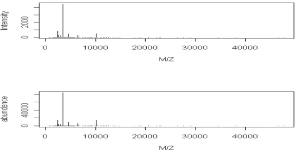
×y.Figure 1 shows the generated intensities in a virtual sample and their correspondent abundances after calibration. We find that there is a substantial change in the scale of vertical axis. The abundance is much larger than the intensity value. Except for the calibration error, the occurrence of isotope and the variability in the experiment are two primary causes for intensity dilution. Table1 includes the intensity and the abundance before and after normalization. The normalization is processed by dividing the intensity or abundance by the total intensity or total abundance of each spectrum. The objective of normalization is to correct for systematic differences in the total amounts on different spectra. A normalized intensity or abundance reflects the relative expression of the protein. Subtracting the normalized abundances by their corresponding normalized intensities, the results are listed in the last column of
Table 1. We find that the differences between original intensities and original abundances are large. An abundance value is about 20 times intensity value. But when compare the normalized values, we find that the trends are quite consistent. The differences are not large, no more than 4.8%. Thus we conclude that the performance of this calibration process is satisfactory.
Figure 1. A virtual sample before/after calibration.
Table 1. Comparison in intensity and abundance with/without normalization.
Protein m/z Intensity Normalized
intensity Abundance Normalized abundance Error in Normalized Values 1 2444.61 823.688 12.043% 14006 10.099% -1.944% 2 2586.39 257.346 3.763% 4444 3.204% -0.558% 3 2966.58 205.269 3.001% 3691 2.661% -0.340% 4 3409.67 4441.053 64.933% 83522 60.225% -4.709% 5 4648.32 423.539 6.193% 8946 6.451% 0.258% 6 6479.38 236.149 3.453% 5796 4.179% 0.727% 7 10117.69 452.358 6.614% 14179 10.224% 3.610% Total 6839.401 138684
2.5 Calibration from Intensity to Abundance
To transfer the intensity of a protein to its abundance, a calibration model is constructed and estimated from a virtual calibration sample. Morris et al. (2005) noted in their supplementary material that this model is built on two empirical observations. The two properties are now verified through the data from the virtual mass spectrometer.
Property 1. Given fixed abundance, the expected inverse intensity of a peak is linear to its mass-to-charge.
Property 2. The intensity of a protein is linear to its abundance.
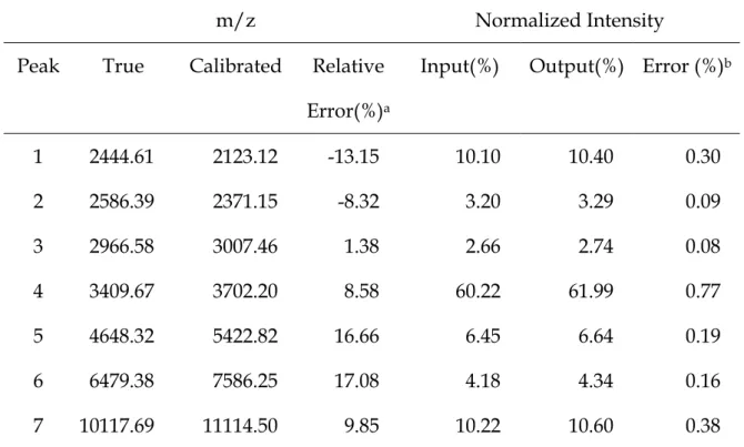
We first choose five points among those present peaks in the virtual sample. Five typical points, which are correspondent to the minimum, the maximum, and the three quantiles of the m/z values, were chosen. For each protein fixed abundance of ions, N, are input to the virtual mass spectrometer. Here N is ranged from 1000 to 10000 with increment 1000. The maximal intensity is a common method for peak quantification and is considered here. Given the abundances, we then obtain five pairs of m/z values and intensities on a spectrum. Figure 2 is the scatter plot of the inverse intensity the five proteins.It’s seen that at fixed abundance the reciprocal intensity increases as m/z increases. Furthermore, the correlation coefficients of 1/intensity and m/z range between 0.98 and 0.99. The trend explains the property 1.
The results of the protein with m/z=3785.642 are plotted in Figure 3. It can be found that as the abundance level increases, the corresponding intensity increases. The correlation coefficients of intensity and abundance are within the range between 0.85 and 0.99. Hence the intensity is linear to abundance. The property 2 is thus verified. We conclude that the two properties are true and the calibration model is adequate.
Figure 2. The scatter plot of 5 selected proteins when N=1000.
Figure 3. The scatter plot of intensity and abundance for the protein with m/z=3785.642.
3 Post-Virtual Spectrometer 3.1 Virtual Mass Spectrometer
The mass spectrometer is an instrument that can measure the masses and relative capacities of proteins. It makes use of the basic magnetic force on a moving charged particle. A biological sample is mixed with an energy-absorbing matrix on a sample plate. While the mixture is crystallized, the crystal is struck with light pulses from a nitrogen laser. The matrix absorbs energy from the laser and transfers it to the proteins, causing the proteins to desorb and ionize. The ionized molecules of proteins are accelerated by an electric field, which is produced by two charged grids, into a drift tube. A detector records the number of ions striking in a fixed time interval. The total flight time for a molecule is then calibrated to m/z and a mass spectrum, with the m/z ratio on the x-axis and the corresponding intensities on the y-axis, is produced.
A virtual mass spectrometer is characterized by a mathematical model, which is established upon physical properties of a real mass spectrometry experiment. In this paper, we consider the virtual mass spectrometer of a linear MALDI/TOF instrument with time-lag focusing or delayed extraction proposed by Coombes et al. (2004) In this instrument an ionized molecule flies through three regions: focusing, acceleration and drift. The mathematical model describes the flight time in each region. The time of flight (TOF) of a molecule to travel from the sample plate to the detector is a sum of flight times in the three regions.
The instrument depends on nine parameters: L, δ, D1, D2, V, V1, τ, µ,σ . L denotes the length of the drift tube, and the default value is 1 meter. δ denotes the delay time, and the default value is 600 nanoseconds. D1 denotes the distance from the sample plate to the first grid. D2 denote the distance between the two grids. The default values of D1 and D2 are 17 mm and 8 mm. For the electric field,
V is the voltage on the sample plate, and V1 is the increasing voltage on the sample plate after the delay. In our simulation, the default value for V is 20,000 volts and 2,000 volts for V1. Each time interval refers to the time resolution of the detector, τ, the default value is 4 nanoseconds. The laser imparts different initial velocities to different particles, and the velocities are modeled as a normal distribution,v0 ~ N(µ,σ2), as suggested by Beavis and Chait(1991). Denoteµ,σ as the mean and the standard deviation of the initial velocities, respectively. Our default values are 350 m/sec forµis 350 m/sec and 50 m/sec for σ .
3.2 Calibration from TOF to m/z
After a biological sample is thrown to the virtual mass spectrometer, one obtains a list of time intervals paired with the numbers of ionized molecules arrived in corresponding time interval. The TOF is then calibrated to mass-to-charge ratio.
Most MALDI-TOF spectra are calibrated externally or internally by running a separate experiment, under the same experimental conditions, using a calibration sample that only contains a small number (typically 5 to 7) of proteins of known mass. The m/z is approximated by a quadratic function of the observed flight time. The unknown coefficients of this quadratic are estimated from the calibration spectrum using least squares; see Coombes et al. (2004). In literature, the time-of-flight (TOF) data is transformed to m/z value via a quadratic equation. For example, Jeffries (2005) stated the following model,
b ) t TOF ( a ) t TOF ( sign V z / m 2 0 0 × × − + − = ,
where V is the known ion voltage and sign(TOF−t.0)=1 for and -1 otherwise, see Jeffries(2005). The and values are determined by a calibration procedure that is performed on a calibrate sample. In this study, we
0 t TOF > b , a t0
use the quadratic model, 2 TOF c TOF b a Z / M = + × + × ,
which was considered by Coombes et al.(2005). Next, the calibration is illustrated by using an example data.
Consider the virtual sample, which consists of 7 peaks, in the previous example of sub-section 2.4. We use 50 proteins with their m/z uniformly ranged from 400 to 20000 Dalton as calibrants. Given abundance N=1000, the TOFs of the calibrants, combined with the known m/z values, are used to estimate the calibration equation. The estimated calibration equation is given by
2 TOF 12) + (3.493e TOF 08) + (3.101e 03) + (6.992e Z / M = + × + × .
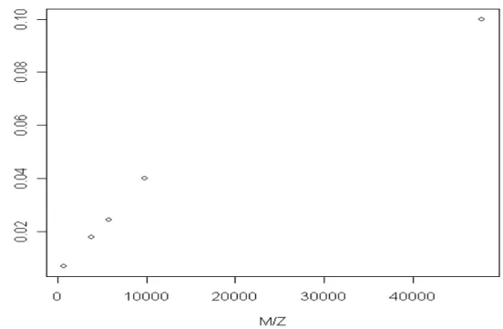
Based on the equation, the raw spectrum is calibrated and the result is displayed in Figure 4 and Table 2. In Table 2, we list the input and output of the 7 peaks. The peak on the spectrum is quantified by using the total intensity. Both the input abundance and the output intensity are normalized by dividing the total number of ionized molecules. We find that the difference between the normalized intensity and the normalized abundance is quite small, at most 0.77%. However, the comparisons in the m/z values show that there is a severe location shift in the mass due to the virtual experiment and the calibration process. The maximal relative error is around 17%, much larger than the conventional declaration in most literature. Next subsection will focus on the problem. The influences of several experimental parameters and the calibration procedure are investigated through an intensive numerical study.
Figure 4. A virtual spectrum before/after calibration.
Table 2. Difference between input and output from the virtual spectrometer
m/z Normalized Intensity
Peak True Calibrated Relative Error(%)a
Input(%) Output(%) Error (%)b
1 2444.61 2123.12 -13.15 10.10 10.40 0.30 2 2586.39 2371.15 -8.32 3.20 3.29 0.09 3 2966.58 3007.46 1.38 2.66 2.74 0.08 4 3409.67 3702.20 8.58 60.22 61.99 0.77 5 4648.32 5422.82 16.66 6.45 6.64 0.19 6 6479.38 7586.25 17.08 4.18 4.34 0.16 7 10117.69 11114.50 9.85 10.22 10.60 0.38
a : Relative Error = {(Calibrated m/z)– (True m/z)}/(True m/z) b : Error = Output – Input.
3.3 Error in Mass
Since the location shift in m/z is a severe problem, we study the effect of several experimental parameters, such as occurrence of isotope, the standard deviation of initial velocity,σ , size of the calibration sample, k, and the length of time resolution, τ . The default settings in the virtual mass spectrometer are σ =50 m/sec, τ =4e-9 second, and k=5 calibrants and considering the existence of isotope.
The mass number of an element is equal to the sum of both protons and neutrons in the nucleus. A single element can have two or more mass numbers due to differences in the number of neutrons that can occur. These different forms of a single element are called isotopes. Because carbon, oxygen, and hydrogen are the elements that make up all organic matter, biologists are often interested in the isotopes of these elements. Each has common and rare forms. The prevalence rates of isotope of carbon, hydrogen and oxygen are 1.1%, 0.02% and 0.4%, respectively. Nitrogen, an important plant nutrient, is also of interest to biologists. There is 0.4% chance of occurrence of isotope.
The occurrence of isotope brings difficulty on peak quantification in intensity and peak identification in m/z. Table 3 is the results that come from several virtual spectra. Each virtual spectrum is generated from the specific virtual population in sub-section 2.4. There are 7 possible peaks in the population. Different parameter settings are employed and listed in Table 4. A relative error is calculated by dividing the difference between the observed m/z and its true m/z by the true m/z. The maximum is chosen among the identified peaks. Fixed other settings, the impact of each factor is investigated. From table 3, we find that the occurrence of isotope, the variability of initial velocity, σ , and the resolution, τ have limited influence on the location shift.
However, the size of calibration sample has noticeable effect. The maximal relative error is reduced from 0.28 to 0.17 when the size is increased from k=5 to k=50.
The following investigations are made upon 1000 virtual spectra. The parameter settings in the example are the σ =50 m/sec, τ =4e-9 second, and k=50 calibrants and considering the existence of isotope. Table 5 studies the existence of pattern in the relative difference between identified m/z and true m/z. The proteins under investigation have m/z values ranged from 2466.72 to 29023.59 Dalton. The mean, standard deviation (SD) and the range among the 1000 identified m/z’s are reported in Table 5. In addition, the last column of the table also gives the relative error, which is calculated by dividing the difference between the mean- and the true-m/z by the true value. From Table 5, we find that as the m/z value increases, the SD and range increase too. There is a greater variation in identifying a heavier protein. The absolute relative error is from 1% to 20%. For small and large m/z, it tends to underestimate the true m/z. The estimation has better performance in 13k-15k.
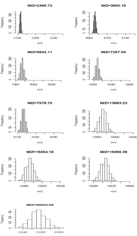
Figure 5 plots the histograms of 1000 identified m/zs for the 9 proteins. Every histogram is approximately bell-shaped and symmetric. We use same scale in the x-axis for all plots. From the figures, with larger m/z, the width of the histogram is found increasing. That confirms our finding on the variation of peak identification in Table 4.
Table 3. Results of virtual spectra under different experimental settings Parameter setting
σ k τ Isotope True m/z Maximal relative error
50a 5a 4e-9a Truea 6578.409 28% 50 5 4e-9 False 1636.104 28% 1 50 4e-9 True 1544.044 38% 5 50 4e-9 True 3801.470 27% 10 50 4e-9 True 4132.737 28% 50 20 4e-9 True 2286.780 33% 50 50 4e-9 True 6479.384 17% 50 100 4e-9 True 6545.029 17% 50 50 1e-9 True 5723.179 17%
a : The default setting
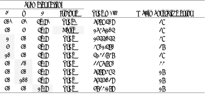
Table 4. Results of identified m/z in 1000 virtual spectra.
Based on 1000 virtual spectra
Protein True m/z
Mean S.D. Range Relative Errora ACTH 18-39 2466.72 2166.88 1.46 9.09 -12% ACTH 7-38 3660.19 4072.46 2.03 12.99 11% RNase A 2+ 6842.11 7974.31 3.27 19.48 17% HBA 2+ 7257.59 8408.60 3.44 22.08 16% HBB 2+ 7978.70 9132.84 3.95 27.27 14% RNase A 13683.23 13972.07 6.81 45.44 02% HBA 15054.18 14971.25 7.35 42.85 -01% HBB 15956.39 15603.79 7.90 49.35 -02% CAH2 29023.59 23274.18 14.04 90.89 -20%
4 Conclusion
In this study, a 5-step simulation design of mass spectra is introduced thoroughly. The five steps include, developing a virtual population, drawing virtual sample from the population, calibrating intensity to abundance, entering the sample to virtual mass spectrometer, and calibrating TOF to m/z. The detail of every step is investigated.
The virtual spectrometer we used here is developed by Coombes et al. (2004) and is for a simple MALDI-TOF experiment with time-lag focusing. The 5-step simulation procedure is shown on Morris et al. (2005). They conducted a simulation study of mass spectrometry to assess a new data preprocessing method.
When the virtual population is decided and the virtual sample is drawn, the calibration which transfers intensity to abundance is employed. In Section Two, the calibration model considered by Morris et al.(2005) is verified and the calibration effect is investigated. We find that the intensities and the calibrated abundances have consistent results when they are adequately normalized.
While a virtual mass spectrum is generated, a calibration is needed to transfer the TOF to mass-to-charge ratio. Another calibration effect which leads to the location shift in m/z is found as a severe problem. Several experimental parameters, such as occurrence of isotope, variation of initial velocity, size of the calibration sample, and length of time resolution, are under investigation in Section Three. In a circumstance with default setting, the relative error in m/z is found .017, maximally. Moreover, when the calibration sample size increases from k=5 to k=50, the relative error achieves the minimum.
In the future, unexpected experimental errors induced during the simulation should be minimized. Determination of adequate parameter settings
is important to design a realistic experiment. In additional to the virtual experiment, the presentation of the generated data heavily depends on data preprocessing step. The parameter setting of preprocessing procedure such that the processed data is more consistent with practical experiment is valuable to strive for. Whenever a mass spectrometry simulation is conducted to assess a data analysis, the deviation inherent in the virtual experiment should be carefully taken into consideration.
Reference
1. Adam, B. L., Qu, Y., Davis, J. W., Ward, M. D., Clements, M. A., Cazares, L. H., Semmes, O. J., Schellhammer, P. F., Yasui, Y., Feng, Z. and Wright, G. L. Jr.(2002)”Serum protein fingerprinting coupled with a pattern-matching algorithm distinguishes prostate cancer from benign prostate hyperplasia and healthy men.” Cancer Research 62, 3609-3614.
2. Coombes, K. R., Koomen, J. M., Baggerly, K. A., Morris, J. S. and Kobayashi, R. (2004) “Understanding the characteristics of mass spectrometry data through the use of simulation,” Cancer Informatics 1, 41-52.
3. Morris, J. S., Coombes, K. R., Koomen, J. M., Baggerly, K. A.and Kobayashi, R. (2005) ”Feature extraction and quantification for mass spectrometry in biomedical applications using the mean spectrum,” Bioinformatics 21, 1764-1775.
4. Bickel, P. J. and Doksum, K. A. (1977) “Mathematical statistics : basic ideas and selected topics”, Holden-Day.
5. Petricoin, E. F., Ardekani, A. M., Hitt, B. A., Levine, P. J., Fusaro, V. A., Steinberg, S. M. and Mills,G. B. (2002) “Use of proteomic patterns in serum to identify ovarian cancer”. Lancet 359 , 572–7.
6. Shiwa, M., Nishimura, Y., Wakatabe, R., Fukawa, A., Arikuni, H., Ota, H., Kato, Y. and Yamori, T. (2003) “Rapid discovery and identification of a tissue-specific tumor biomarker from 39 human cancer cell lines using the SELDI ProteinChip platform.” Biochem Biophys Res Commun 309(1), 18-25.
7. Vorderwülbecke, S., Cleverley, S., Weinberger, S. R. and Wiesner, A. (2005) “Protein quantification by the SELDI-TOF-MS–based ProteinChip® System.”