Parallel 4×4 2D transform and inverse transform architecture for MPEG-4 AVC/H.264

(1)

PARALLEL 4 x 4 2D TRANSFORM AND INVERSE TRANSFORM ARCHITECTURE FOR

MPEG-4 AVUH.264

Tu-Chih Wung,

Yu-

Wen Huang. Hung-Chi Fang, and Liang-Gee Chen

DSP/IC

Design Lab, Graduate Institute

of

Electronics Engineering,

Department

of

Electrical Engineering, National Taiwan University, Taipei, Taiwan

{eric,

yuwen, honchi, lgchen} @video.ee.ntu.edu.tw

ABSTRACT

Transform coding has been widely used in video coding standards. In this paper. a hardware architecture for accelerating transform coding operations in MPEG-4 AVC/H.264[2] is presented. This architecture calculates 4 inputs in parallel by the fast algorithms described in [4]. The transpose operations are implemented by a register array with directional transfers. This architecture has been mapped into a 4 x 4 multiple transforms unit and synthesized in

TSMC 0.35um technology. The multiple transform processor can process 320M pixeldsec at SOMhz for all 4 x 4 transforms used in MPEG-4 AVC/ H.264.

1. INTRODUCTION

MPEG-4 AVUH.264 is initiated by ITU-T as H.26L and will be- come a joint standard for ITU-T and MPEG. The compression gain of H.264 is much higher than H.263[1] and MPEG-4 simple profile. One of the major differences between H.263 and H.264 is the transform coding. H.264 adopts variable block size motion compensation scheme and the smallest block size is 4 x 4 pixels,

Transform coding for residual coding is set to 4 x 4 to match the smallest block size. Although the transform coding gain decreases a little comparing to 8 x 8 DCT[3] in H.263, good motion estimation results in better PSNR performance.

Another advantage of H.264 transform coding is the simplic-

ity of the transform. Integer coefficient transform, which is a close approximation to DCT, is adopted i n H.264. Since the coefficients are integers, there will be no mismatch problem like H.263, and the restriction of intra update in H.263 is removed. Integer coefficients also imply simple hardware implementation. H.264 only use 4 coefficients for the transforms. And the multiplications can be replaced by shifts and additions.

Although the computation complexity ofthe transforms in the H.264 standard is less than H.263, hardware implementation of the transform coding is required in both dedicated and platform based codec systems. Dedicated hardware design of codec requires transform unit to complete the dataflow. Platform based design usually requires transform unit as a coprocessor to increase the processing rate and alleviate the loading of the processor. In

this paper, we propose a parallel architecture to increase the data processing rate in the transform unit. The architecture can process 4 pixels per cycle with a small gate count. The interface bit width is 64 bits so that it can be easily adapted to many existing buses.

This paper is organized as follows. H.264 transform algorithms are described in section 2. Our proposed architecture is

Header

J

-

7

vi

Figure I : Block diagram of H.264 encoding flow

illustrated in section 3. Section 4 shows the dynamic range analysis for each transform. A multi-transform processor design which can execute all 4 x 4 transforms in H.264 is shown in section 5. Implementation result and the comparison with other DCT archi- tectures are shown in section 6. Finally, a conclusion is given in section 7.

2. TRANSFORM CODING IN H.264

Fig. I shows the encoding flow of H.264, which is a hybrid coder similar to H.263. The input frame is divided into macroblocks

(MBs) of 16 x 16 pixels. Each MB performs spatial and temporal prediction to find the best predictor in the spatial and temporal do- main. The spatial prediction is also called intra prediction. There are two types of intra prediction in H.264. One is 4 x 4 intra prediction and the other is 16 x 16 intra prediction. The temporal prediction is the multiple reference frame and variable block sizc motion estimation. Its prediction precision is quarter pixel in the

baseline profile. The residual MB is then obtained by subtracting predictor from the original.

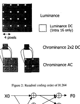
The residual MB is coded as Fig.2. It is funher divided into sixteen 4

x

4 blocks for luminance and 4 blocks for chrominance. If the 16 x 16 intra prediction mode is chosen for the MB. the DC terms of the luminance blocks are extracted lo form a 4

x

4 block. Hadamard transform is then applied on it. The DC terms

of

the chrominance blocks are also extracted to 2

x

2 blocks. A 2 x 2 transform is used for these DC terms for block number 16 and 17

in Fig.2.

There are two types o f 4 x 4 transforms for the residual coding. The first one is for luminance residual blocks. The transform and

II-800

(2)

t,

4 pixels

Chrominance

2x2

DC

Figure 2 ; Residual coding order of H.264

xo

FO

x1

F2

x2

F1

x3

F3

Figure 3: Fast algorithm of 4 x 4 forward transform for residual blocks

inverse transform matrices are shown in 3 . 1 and Eq.2. Their fast algorithms are shown in Fig.3 and Fig.4. The transform matrix only contains 4 coefficients,l,-1,2,-2, which can he implemented by shifters and adders. The fast algorithm in Fig.3 further reduces the number of the addition from 16 to 8 with butterfly operations. The inverse transform is very similar to the forward transform and the complexity is the same. Note that the inverse transform matrix is scaled inverse of the transform matrix. W e scaling is done by the quantization and dequantization steps.

FO 1 1 1 1

xo

[

::]

=[I

-:

-2

r:

2 -:]

-1

[

::]

x3

(1) F 3 XO, 1 1 F'O x3, -1

The other type of the transform is Hadamard transform. It is applied to the luminance DC terms in 1 6 x 16 intra prediction

F'O

X'O

F'2

x'1

F'1

X'2

F'3

x'3

Figure 4 Fast algorithm of 4 x 4 inverse transform for residual blocks

xo

FO

x1

F2

x2

F1

x3

F3

Figure 5 : Fast algorithm of 4 x 4 Hadamard transform for residual Mocks

mode. The transform matrix is shown in Eq.3 and the fast implementation is given in Fig.5. W e Hadamard transform is a sim- plified version of Eq.1 by replacing the coefficient 2 by I . The inverse Hadamard transform is simply the transpose of Eq.3 since Hadamard transform is orthogonal. Because the transform matrix is symmetric, the inverse Hadamard transform is the same as the forward transform. The Hadamard transform matrix is also scaled. The scaling factor is 4 for each 2D transform.

r F o i

r i 1 I

i i r x o i

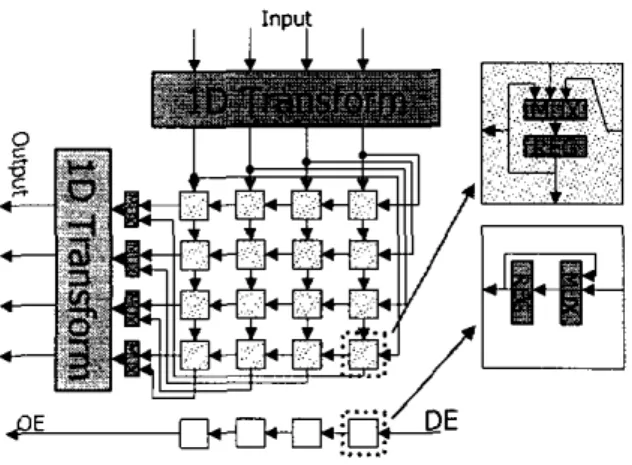
3. PROPOSED PARALLEL ARCHITECTURE

The proposed parallel architecture is shown in Fig.6, which contains two I D transform units and a transpose register array. The ID

transform unit is implemented by using fast algorithm data flow like Fig.3,4 and 5 . Since the fast algorithm only contains shift and addition operations, the I D transform operation is designed to he completed within one cycle. Note that the shift operations in the hardware implementation are done by wirings. No delay or area will be introduced in the shift operations.

The transpose register element consists of a three input multiplexer and a register. The multiplexer controls the data flow of the transpose register array. The first input of the multiplexer is a self feedback from the register. It is used for "no operation"(N0P)

(3)

range of 1 bit. The I D transform outputs,

FO

- El, should be 12 hits because there are some components doubled before additions. The transpose register array hit width is determined by the first I D transform output. So the bit width of the transpose register array is thus 12 hits.

The dynamic range of the I D forward transform increases 3

bits from the discussion above. The input bit width of the second I D transform is 12 bits from the transpose register array and the output should be 15 bits.

4.2. 4 x 4 inverse transform for residual block

The input of the inverse transform is from the inverse quantiza- tion function. The specification of H.264 only guarantees that 16 bits arithmetic is enough. But if we further investigate the transform and quantization algorithms in H.264. we will find that the dynamic range of the inverse quantization output is 15 bits since the quantizatiodinverse quantization scaling factor is less than 1.

In the 4 x 4 inverse transform implementation, there is one

extra thing needed to be done in the output stage. H.264 states that the reconstmction value should be shifted right by 6 bits with rounding. This operation requires additional four adders to do the rounding operations.

4.3. Hadamard transform

The input of the Hadamard transform is the DC coefficients after quantization. The quantization of the DC terms in 16 x 16 in- tra mode is different to other modes. It preserves two extra bits comparing to other modes. The smallest quantization parameter

(QP) has an equal effect of dividing by

IO,

which reduces 3 bits of dynamic range in the normal mode. Since two extra bits are preserved in 16 x 16 intra mode. the dynamic range of the input

is 15-3+2=14 hits. The I D Hadamard transform will increase dy- namic range by 2 hits, so the transpose register array should be implemented with 16 bits.

S. MULTIPLE FUNCTION TRANSFORM PROCESSOR DESIGN

In H.264 encoding scheme, the computation complexity of the transform is about double of the pixel rate (forward and inverse transforms). The processing speed of our proposed parallel architecture is much higher than the existing video format. In order

tn reduce the gate count required for the three different transform processors, we combine the three transform units into one multiple function transform processor which can execute all the three transform operations in H.264.

In

our proposed architecture shown in Fig.6. the

1D

transform

can he any type of the transform. If a reconfigurable I D transform unit which can he configured to one of the three transforms in H.264 is applied, the architecture can be extend to a multiple function transform processor.

By the observation of Fig.3 to 5 , we can find that every

1D

transform contains 8 arithmetical operations. And Hadamard transform can he achieved by removing the scaling factor, which can be easily done by multiplexers. In order to get a clear view of how to achieve multiple transforms in a single design, we overlap Fig.3.4

e

2

t t t t

-E

...,

. .

$E

...

Figure 6: Proposed parallel transform architecture

condition. The second input of the multiplexer is the data from the upper register element. The third input is the data from the right, If all of the multiplexers select the data from the upper register elements. the data in the register array will be shift down. The bot- tom row of the register array will be outputted to the second I D transform unit as the left transform pan of FigS. However, if the multiplexers select the data from the right, the data will be shift to the left and the leftest column of the register array will be sent

to the second I D transform unit. The direction of the transpose register array is controlled by a simple counter which counts valid inputs by data enable(DE) signal. The direction will be changed every four valid input clocks so that the transpose operation can he done i n this register array.

Our proposed architecture has a fixed latency of 4 clock cy- cles. Unlike the serial architecture described in [SI. this proposed archilcclure can output data even the next block data is not contin- uously inputted.

This

feature is done by preserving the data valid status in the register array. The registers on the bottom row of Fig.5 are built for this function. The registers preserve the latest four input data enable signals for the output enable (OE) signal. The feedback loop is used for NOP condition, which is the same as the signal for the transpose register array. The condition of NOP happens when data counter

#

0 and DE = 0, which implies input

data transfer break within a block. Since the transpose register file changes direction when all the data arc filled, the data transfer break within a block will result in a stall cycle.

4.

BIT WIDTH ANALYSIS

The bit width requirements of these three transform matrices in H.264 are not the same. By assigned the lowest required bit widths to datapath and registers, the gate count and timing can be opti- mized. The detail analysis is given in the following subsections.

4.1. 4 x 4 transform for residual block

The input of the forward transform is the residual block. The dy. namiciange of the residual is from -256 to +255, i.e. 9 bits. From Fig.3, the bit width of the first column adder outputs should be 10

bits since addition and subtraction operations increase the dynamic

and 5 togethir. The overlapped dataflow figure is shown in Fig.7. In Fig.7, all the adders have three inputs. It means that a common input which is not changed by the transform type exists. So only

(4)

xo

x1

x 2

x 3

YO

Y2

Y1

Y3

Figure 7: Overlapped data flow of three fast algorithms

one of the two inputs in the 8 adders is required lo be selected by the multiplexers. The multiplexers are controlled by the transform selection control bits of the input. Moreover, 3 out of 8 adders are replaced by an adderlsubtractor. which can dynamically change its functionality from an adder to a subtractor.

The bit width of all the arithmetical parts and registers is set to 16 since the maximum bit width of the three transforms is 16. One extra output stage which implements the rounding and shift- ing operations in the inverse transform is added after the output of the second I D transform. This stage can be bypass for the other two transform configurations.

The configuration bits for the first I D transform are preserved like the DE signals in Fig.6 for the fast switching between two transform matrices. By preserving these configuration bits, the two ID transform modules can perform different transforms at the same time. The type for the second 1D transform is always correct since the configuration bits and input data are synchronously fed

into the register array.

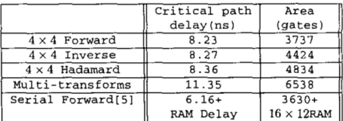
6. IMPLEMENTATIONS AND COMPARISON HDL design flow is used to reduce design period and provide technology independent portability. The three 4 x 4 transforms for H.264 have been mapped in our proposed parallel architecture and synthesized in TSMC 0 . 3 5 ~ technology. The gate count and de- lay are listed in Table l . In order to compare the implementation results to serial versions of the transform architecture, shrinking down version of 151 is also implemented. This architecture is more than three times faster than [SI, and also smaller when RAM area is included.

The multiple transform processor implementation is slower and bigger than the dedicated design. The processing speed can be achieved to 320M pixelslsec at 80Mhz. It is sufficient for the existing video formats including HDTV formats. The area of the multiple transform processor is less than the sum of three transform units. It is a cost efficient accelerator solution for platform based video codec design.

7. CONCLUSIONS

In this paper. we propose a high speed, parallel transform architecture for MPEG-4 AVClH.264. Forwardlnverse transforms for residual block and DC terms can be mapped

to

this architecture. The architecture could process four pixels per clock cycle. We have mapped three transform matrices used in MPEG-4 AVUH.264 to TSMC 0 . 3 5 ~ technology. The processing speed can achieve

Table 1: Implementation results of our proposed parallel architec- tures and serial architecture

I

11

Critical path

I

Area

I/

delay (ns) (gates) 4 x 4 Forward 4 x 4 Inverse 4 x 4 Hadamard 8.36 Multi-transforms 11.35 Serial Forward151 6.16+

I

. .

I(

RAM Delay

I

16 x 12-

I

500 Msampledsec for all of the three transform matrices. This proposed architecture is very compact; for the 4 x 4 forward transform, the gate count is only 3737. Comparing to other serial archi- tectures, it has better timing-area property. We also implemented a multiple function transform processor which can process all the

4 x 4 transforms in MPEG-4 AVClH.264. This architecture can be applied to a hardware accelerator or dedicated hardware design for MPEG-4 AVCiH.264 video codec.

8. REFERENCES

[ I ] Draft ITU-T Recommendation H.263, Video coding for low

bitrate communication, ITU-T, 1997.

[2] T. Wiegand. "Working draft for recommendation H.264", Joint Video Team(1VT) of ISOIIEC MPEG and ITU-T VCEG, Doc. JVT-C167, May, 2002. Available at ftp://ftp.imtc- Rles.org/jvt-experts.

131

K. R.

Rao

and

P.

Yip, Discrete Cosine TransfomxAlgorithms. Advantages. Applications. Boston: Academic Press. 1990.

[4] H. Malvar, A. Hallapuro, M. Karczewicz. and L. Kerof- sky, "Low-complexity transform and quantization with 16-

bit arithmetic for H.26L", Proceeding of lClP 2002, vol. 2, pp.489-492, Rochester, NY, Sept. 2002.

151 A. Madisetti and A.N. Willson, "A 100 MHz 2-D 8 x 8

DCTIIDCT processor for HDTV applications", IEEE Trans-

action on Circuits and Systems for Video Technology, vol. 5 .

no. 2,pp. 158-165,Apr., 1995.

[6] A. Hallapuro,

M.

Karczewicz, and

H.

Malvar, "Low complexity transform and quantization", JVT of ISO/IEC MPEG and ITU-T VCEG, Docs. JVT-BO38 and JVT-BO39, Jan. 2002. [7] A. Hallapuro,

M.

Karczewicz, "Low complexity (I)DCT',

ITU-T SG16 Doc. VCEG-N43, Sept., 2001.

[81 H.

S.

Malvar. "Low-Complexity length-4 transform and quantization with 16-Bit arithmetic", ITU-T SG16 Doc. VCEG- N44, Sept., 2001.