在磁場中, 於一存在位能障的量子通道中的同調傳輸

全文

(1)Coherent transport through potential barriers in a quantum channel in magnetic field Student: Yu-yu Lin. Advisor: Chon-Saar Chu. Department of Electrophysics National Chiao-Tung University. January 19, 2006.

(2) Abstract In this thesis, we try to push our theoretical description of magnetotransport in a quantum wire to the high magnetic field regime. Two different approaches, namely, the mode matching approach and the partial Fourier transformation of the Lippmann-Schwinger equation approach, have been employed to cross check our results. We have plotted the transmission, the wavefunction, and the current density patterns and have interpreted them in light of the edge states. A simple criteria for the formation of edge states is reached, which is arisen from the comparison of the cyclotron radius and the effective width of the wire. For the case of a single repulsive barrier, a transmission dip is found at the threshold of a subband. For the case of a single attractive barrier, two transmission dips are found for incident energy that lies below a subband threshold. These are discussed in terms of the edge states and the evanescent modes.. i.

(3) 摘要在本論文中, 我們試著將所能得到的在量子導線的磁導率增促到高磁場的範圍。我們使用了兩種不同的方法、模態匹配近似法及 Lippmann-Schwinger 方程式的部分富立葉轉換近似方法、來交互比對確定我們的結果。接著我們對對穿透率、波函數、及電流密度作圖並解釋其中邊緣態的現象。經由比較比較磁場的迴旋半徑及通道的等效寬度, 提供了一個簡單度量邊緣態產生的方法。在通道含有一個排斥力的雜質時, 我們在次能帶底部之上可以發現一個凹陷。而在吸引的雜質時, 則在入射能量低於次能帶底部的地方發現兩個凹陷。我們也會討論邊緣態跟衰減態的現象。. ii.

(4) 誌謝從專題研討開始, 至今也已經四年有了。面對老師的時間, 也不可所謂不長。除了在專業上的指導與討論, 更應該感謝的是由老師本身所傳達的對學問的專注與熱情。尤其是在做學問的態度上, 我能學的實在太多也得到太多。除了老師, 也該感謝在這日子裡不斷給予指導叮嚀的唐志雄學長。總是能在我需要協助的時候, 給予最好的建議。當然, 伙伴是不能少的。從老王學長、淑維學姊到哲明、宇廷、靖航、淑娟及其他的朋友們。有你們的出現、陪伴才不會那麼孤單。尤其, 要特別感謝老王學長, 在實驗室裡的這段日子真的是多受到照顧了。另外, 也要感謝許永昌學長及 Prof. Vidar Gudmundsson 的討論, 特別是在數值程式方面的指導, 這在我的研究上提供了最有力的協助。最後, 我要感謝我的家人, 這也是之於我最重要的支持力量。不管多麼困難, 你們總是永遠無私的付出與體諒。感謝所有。. iii.

(5) Contents Abstract in English. i. Abstract in Chinese. ii. Acknowledgement. iii. Contents. vi. List of Figures. xii. 1 Introduction and background. 1. 2 Introduction to Landauer-B¨ uttiker formula and our physical model. 6. 2.1. Landauer-B¨ uttiker formalism . . . . . . . . . . . . . . . . . . . . . . . . . .. 6. 2.2. Our physical model and formulation . . . . . . . . . . . . . . . . . . . . . .. 9. 3 Mode-matching (MM) method. 14. 3.1. Formalism . . . . . . . . . . . . . . . . . . . . . . . . . . . . . . . . . . . . 14. 3.2. Normalization constant and evanescent mode . . . . . . . . . . . . . . . . . 17. 3.3. Mode-matching approach . . . . . . . . . . . . . . . . . . . . . . . . . . . . 20. 3.4. Current density and conservation condition . . . . . . . . . . . . . . . . . . 26. 3.5. Numerical results . . . . . . . . . . . . . . . . . . . . . . . . . . . . . . . . 29. 3.6. Summary and discussions . . . . . . . . . . . . . . . . . . . . . . . . . . . 32. iv.

(6) CONTENTS 4 An approach of partial Fourier transformation of the Lippmann-Schwinger (PFTLS) equation. 36. 4.1. Formalism . . . . . . . . . . . . . . . . . . . . . . . . . . . . . . . . . . . . 37. 4.2. Scattering matrix method . . . . . . . . . . . . . . . . . . . . . . . . . . . 43. 4.3. Wavefunction and current density . . . . . . . . . . . . . . . . . . . . . . . 46. 4.4. Numerical results . . . . . . . . . . . . . . . . . . . . . . . . . . . . . . . . 48. 4.5. Summary . . . . . . . . . . . . . . . . . . . . . . . . . . . . . . . . . . . . 52. 5 Comparing the numerical results from the MM and PFTLS approaches 54 5.1. Transmission . . . . . . . . . . . . . . . . . . . . . . . . . . . . . . . . . . 54. 5.2. Wavefunction and current pattern . . . . . . . . . . . . . . . . . . . . . . . 59. 5.3. Summary . . . . . . . . . . . . . . . . . . . . . . . . . . . . . . . . . . . . 61. 6 Magnetoconduction in quantum channel with a repulsive barrier. 62. 6.1. Tuning of the magnetic field . . . . . . . . . . . . . . . . . . . . . . . . . . 62. 6.2. Tuning of the barrier strength . . . . . . . . . . . . . . . . . . . . . . . . . 63. 6.3. Analyses of numerical results and physical interpretations . . . . . . . . . . 64. 6.4. Summary . . . . . . . . . . . . . . . . . . . . . . . . . . . . . . . . . . . . 70. 7 Magnetoconduction in quantum channel with an attractive barrier. 73. 7.1. Tuning of the magnetic field . . . . . . . . . . . . . . . . . . . . . . . . . . 73. 7.2. Tuning of the barrier strength . . . . . . . . . . . . . . . . . . . . . . . . . 75. 7.3. Analyses of numerical results and physical interpretations . . . . . . . . . . 79. 7.4. Summary . . . . . . . . . . . . . . . . . . . . . . . . . . . . . . . . . . . . 87. 8 Concluding remarks. 89. 9 Possible future works. 92. 9.1. Double and multiple barriers . . . . . . . . . . . . . . . . . . . . . . . . . . 92. A Detail of the integrations. 97 v.

(7) CONTENTS. Appendix A.1 A.2 A.3 A.4 A.5 A.6 A.7 A.8. R R R R R R R. 97. φom (y)φ± n (y)dy . . . . . . . . . . . . . . . . . . . . . . . . . . . . . . . . . 99 φsm (y)φ± n (y)dy . . . . . . . . . . . . . . . . . . . . . . . . . . . . . . . . . 102 ∗. ± φ± m (y)φn (y)dy . . . . . . . . . . . . . . . . . . . . . . . . . . . . . . . . 103. φom (y)Vs (y)φ± n (y)dy . . . . . . . . . . . . . . . . . . . . . . . . . . . . . . 105 φsm (y)Vs (y)φ± n (y)dy . . . . . . . . . . . . . . . . . . . . . . . . . . . . . . 109 ∗. ± φ± m (y)Vs (y)φn (y)dy. . . . . . . . . . . . . . . . . . . . . . . . . . . . . . 112. ∗. ± yφ± n φn dy = ±Re[αn ] . . . . . . . . . . . . . . . . . . . . . . . . . . . . . 115. R∞. −∞. φom ∗ (y)Vs (y)φon (y)dy . . . . . . . . . . . . . . . . . . . . . . . . . . . . . 116. A.9 Recurrence relations of Hermite polynomial R 2 A.10 e−x Hm (ax)Hn (bx)dx . . . . . . . . . . . . R 2 A.11 e−x Hm (x + a)Hn (x + b)dx . . . . . . . . . R 2 A.12 e−(x−y) Hm (αx)Hn (αx)dx . . . . . . . . .. Bibliography. . . . . . . . . . . . . . . . . . 117 . . . . . . . . . . . . . . . . . 118 . . . . . . . . . . . . . . . . . 120 . . . . . . . . . . . . . . . . . 122. 123. vi.

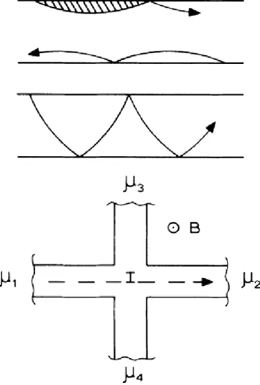
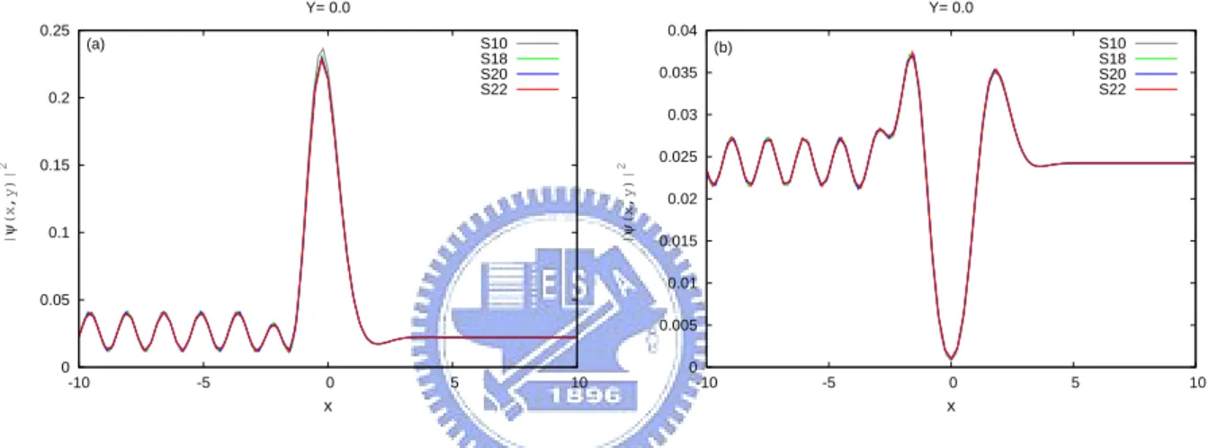
(8) List of Figures 1.1. Top: Skipping orbits, corresponding to edge states. Center: Traversing trajectory, corresponding to a traversing state(hybird magnetroelectric subband). Bottom: Four-terminal conductor for Hall-resistance measurement. (C. W. J. Beenakker and H. van Houten, Phys. Rev. Lett. 60, 2406 (1988)). 2.1. The figure of our system.. 3.1. Compare the numerical results of three basis sets. The red line is the result. 4. . . . . . . . . . . . . . . . . . . . . . . . . . . . 10. s projected to φ± m (y, km ); the green one is projected to φm (y); and the blue. one is projected to φom (y). The strength of the impurity barrier is repulsive with 1.0E ∗ in (a) and attractive with −1.0E ∗ in (b). . . . . . . . . . . . . 30 3.2. Changing the number of subband Nc to check the saturation and the accuracy break down of the numerical calculation. We fix the incident energy at E = 7ωy E ∗ , the strength of the impurity barrier is 1.0E ∗ . . . . . . . . . 31. 3.3. The saturation of transmission versus Nc from 26 to 30 for B = 1.0 and the strength of impurity barrier is repulsive with 1.0E ∗ in (a) and attractive with −1.0E ∗ in (b). . . . . . . . . . . . . . . . . . . . . . . . . . . . . . . . 33. 4.1. The saturation versus the numbers of subband Nc for a repulsive barrier with 1.0E ∗ in (a) and an attractive barrier with −1.0E ∗ in (b). The incident energy is at 7ωy E ∗ .. . . . . . . . . . . . . . . . . . . . . . . . . . . . . . . 49. vii.

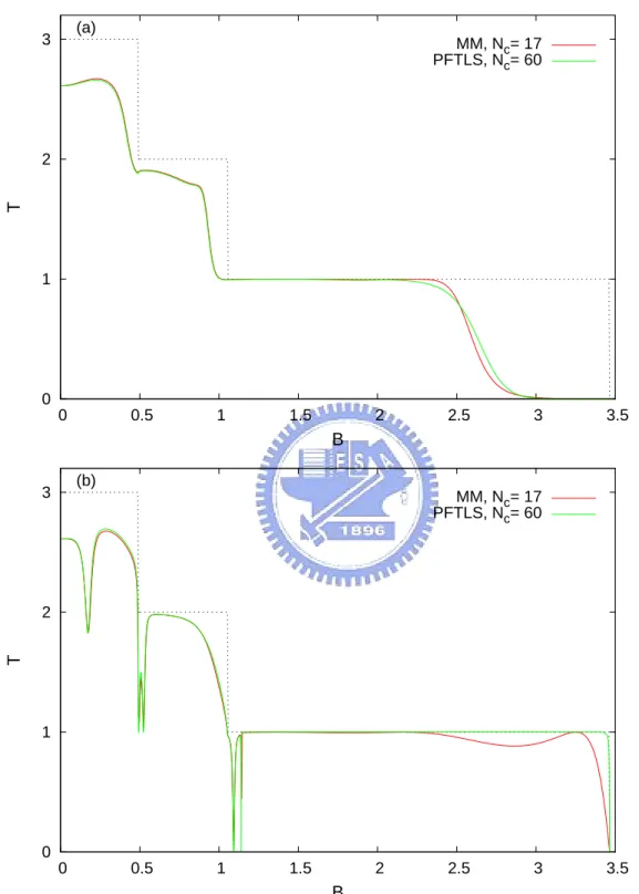
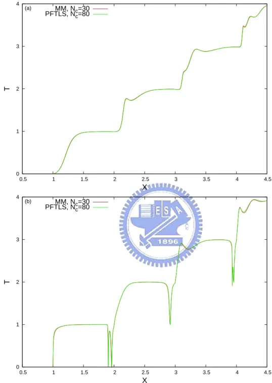
(9) LIST OF FIGURES 4.2. The saturation versus the number of subband for repulsive barrier with 1.0E ∗ in (a) and −1.0E ∗ in (b). And the amplitude of the magnetic field is 1.0B ∗ .. 4.3. . . . . . . . . . . . . . . . . . . . . . . . . . . . . . . . . . . . . 50. The saturation versus the number of subband for repulsive barrier with 1.0E ∗ in (a) and −1.0E ∗ in (b). And the amplitude of the magnetic field is 2.0B ∗ .. 4.4. . . . . . . . . . . . . . . . . . . . . . . . . . . . . . . . . . . . . 50. The probability density of |ψn (x)|2 as a function of coordinate variable x for various Nc from 10 to 22, incident energy is 1.4ΩE ∗ and the amplitude of magnetic field is 1.0. The barrier is repulsive in (a), and attractive in (b). 51. 4.5 The saturation of the wavefunction of PFTLS approach. We plot the wavefunction of −10 < x < 10 and x = 0 for various numbers of subbands, 10, 18, 20, and 22, and the incident energy X = 1.6, the amplitude of magnetic field is 1.0, and the strength of the barrier is repulsive, 1.0 in (a), and attractive, −1.0 in (b). 5.1. . . . . . . . . . . . . . . . . . . . . . . . . . . . . 52. The transmission versus the amplitude of magnetic field of the two approaches, MM and PFTLS. we fix the incident energy at 7ωy E ∗ which X = 3 and the barrier strength is repulsive with 1.0E ∗ in (a) and attractive with −1.0E ∗ in (b). . . . . . . . . . . . . . . . . . . . . . . . . . . . . 55. 5.2 The transmission versus the incident energy X of the two approaches, MM and PFTLS. The magnetic field amplitude is 1.0B ∗ and the strength of the repulsive barrier is V0 = 1.0E ∗ in (a) and the attractive barrier is V0 = −1.0E ∗ in (b). 5.3. . . . . . . . . . . . . . . . . . . . . . . . . . . . . . . 57. Comparing the saturation of the two approaches by plotting the transmission versus the incident energy, the magnetic field amplitude is B = 0.5B ∗ and the strength of the impurity barrier is V0 = −1.0E ∗ . And we enlarge one part of figure (a) from 1.8 to 2.01 in (b). . . . . . . . . . . . . . . . . . 58. viii.

(10) LIST OF FIGURES 5.4. Compare the wavefunction of the two approaches, MM and PFTLS, for −10 < x < 10 and y = 0. The incident energy X = 1.6, and the strength of the barriers are repulsive and 1.0 in (a) and (c), attractive and −1.0 in (b) and (d), and the amplitude of the magnetic field are 0.1 in (a) and (b), 0.2 in (c) and (d).. 5.5. . . . . . . . . . . . . . . . . . . . . . . . . . . . . . . . 58. The current density in the wire with magnetic field, B = 0.15B ∗ , and the incident energy is X = 1.9 which is close to the subband bottom of second subband. And the strength of the barrier is repulsive, 20. (a) is the current density by using the approach of MM, and (b) use the approach of PFTLS. 60. 6.1. The transmission versus the incident energy and incident from the first subband for various amplitudes of the magnetic field form 0.0B ∗ to 2.0B ∗ and the strength of the repulsive barrier is V0 = 1.0E ∗ . The dips structure happen above X = 2 and X = 3 . . . . . . . . . . . . . . . . . . . . . . . . 63. 6.2. The transmission versus the incident energy and incident from the second subband for various amplitudes of the magnetic field form 0.0B ∗ to 2.0B ∗ and the strength of the repulsive barrier is V0 = 1.0E ∗ . The valleys structures happen just above the integral X . . . . . . . . . . . . . . . . . 64. 6.3. The transmission versus the incident energy and incident from the first subband for various strength of repulsive barrier from 0.0E ∗ to 1.4E ∗ and the amplitude of the magnetic field is 2.0B ∗ .. 6.4. . . . . . . . . . . . . . . . . 65. The total wavefunction and the current density patterns in the wire with a strong repulsive barrier V0 = 20E ∗ , the amplitude of the magnetic field is 1.0B ∗ , and the incident energy is X = 1.7 from the first subband.. ix. . . . 66.

(11) LIST OF FIGURES 6.5. Top: The total wavefunction and the current density patterns of the strength of the repulsive barrier is V0 = 1.0E ∗ , the amplitude of magnetic field is B = 0.5B ∗ , and the incident energy is X = 1.8 from the first subband; Left of bottom: The wavefunction and the current density components of the first subband; Right of bottom: The wavefunction and the current density components of the second subband.. 6.6. . . . . . . . . . . . . . . . . . . . . . 67. Top: The total wavefunction and the current density patterns of the strength of the repulsive barrier is V0 = 1.0E ∗ , the amplitude of magnetic field is B = 0.5B ∗ , and the incident energy is X = 2.2 from the first subband; Left of bottom: The wavefunction and the current density components of the first subband; Right of bottom: The wavefunction and the current density components of the second subband.. 6.7. . . . . . . . . . . . . . . . . . . . . . 68. Top: The total wavefunction and the current density patterns of the strength of the repulsive barrier is V0 = 1.0E ∗ , the amplitude of magnetic field is B = 0.5B ∗ , and the incident energy is X = 2.8 from the first subband; Left of bottom: The wavefunction and the current density components of the first subband; Right of bottom: The wavefunction and the current density components of the second subband.. . . . . . . . . . . . . . . . . . . . . . 69. 6.8 Top: The total wavefunction and the current density patterns of the strength of the repulsive barrier is 1.0, the amplitude of magnetic field is 0.5, and the incident energy is X = 2.2 and incident from the second subband; Left of bottom: The wavefunction and the current density components of the first subband; Right of bottom: The wavefunction and the current density components of the second subband.. . . . . . . . . . . . . . . . . . . . . . 71. 7.1 The transmission versus the incident for various amplitudes of magnetic field from 0.0 to 2.0, and the strength of the impurity barrier is 1.0.. x. . . . 74.

(12) LIST OF FIGURES 7.2. The position in energy X of the dip structure in the transmission curve versus the amplitude of magnetic field; the strength of the impurity barrier is 1.0E ∗ in (a) and 1.4E ∗ in (b). . . . . . . . . . . . . . . . . . . . . . . . . 76. 7.3. The transmission as a function of X for various strength of impurity barrier from 0.0 to −2.0E ∗ . The magnetic field is 0.2B ∗ . . . . . . . . . . . . . . . 77. 7.4. The transmission as a function of X for various strength of impurity barrier from 0.0 to −2.0E ∗ . The magnetic field is 1.0B ∗ . Plotting Fig(a) again of energy range at 1.7 to 2.1 in Fig(b).. . . . . . . . . . . . . . . . . . . . . . 78. 7.5. The relation of the position of the first dips with V0 . . . . . . . . . . . . . . 79. 7.6. The wavefunction and the current density patterns at the first dip with B = 0.4, Top: the total wavefunction and current density patterns in the wire; Left of bottom: the contribution of the propagating mode; Right of bottom: the contribution of the evanescent mode. . . . . . . . . . . . . . . 80. 7.7. The wavefunction and the current density patterns at the second dip with B = 0.4, Top: the total wavefunction and current density patterns in the wire; Left of bottom: the contribution of the propagating mode; Right of bottom: the contribution of the evanescent mode. . . . . . . . . . . . . . . 81. 7.8. The wavefunction and the current density patterns at the dip structure with B = 0.7, Top: the total wavefunction and current density patterns in the wire; Left of bottom: the contribution of the propagating mode; Right of bottom: the contribution of the evanescent mode. . . . . . . . . . . . . . 82. 7.9 The wavefunction and the current density patterns at the first dip with B = 1.0, Top: the total wavefunction and current density patterns in the wire; Left of bottom: the contribution of the propagating mode; Right of bottom: the contribution of the evanescent mode. . . . . . . . . . . . . . . 83. xi.

(13) LIST OF FIGURES 7.10 The wavefunction and the current density patterns at the second dip with B = 1.0, Top: the total wavefunction and current density patterns in the wire; Left of bottom: the contribution of the propagating mode; Right of bottom: the contribution of the evanescent mode. . . . . . . . . . . . . . . 84 9.1. Two embedded δ-type barrier in the wire which the distance between them is 2.0a∗ , and we plot the transmission as a function of incident energy X for various amplitude of magnetic field from 0.0B ∗ to 1.0B ∗ , and the strength of the two barrier are both 1.0E ∗ in (a) and −1.0E ∗ in (b).. 9.2. . . . . . . . . 94. The transmission versus the incident energy for double embedded impurity barrier which the strength is 1.0E ∗ in (a) and −1.0E ∗ in (b), the distance between the two barrier is changed for various distance from 2.0a∗ to 4.0a∗ . 95. 9.3. The transmission of the first channel versus the incident energy for 25 slices of δ-type barrier and the distance between two near slices is 3.0a∗ . We change the amplitude of magnetic field from 0.0B ∗ to 0.4B ∗ in series of these five figures.. . . . . . . . . . . . . . . . . . . . . . . . . . . . . . . 96. xii.

(14) Chapter 1 Introduction and background The discovery of the quantized conductance steps in two-dimensional electron gas(2DEG), micro-constrictions based on GaAs/Alx Ga1−x As heterostructures [1,2], the quantized conductance steps followed an increase of interest in the study of quantum ballistic transport through narrow channels in 2DEG [3]. In particular, the influence of impurities on the conductance attracted a great deal of attention since impurities inside or near the conducting channel may destroy the conductance quantization [4–21], The effect of the impurities is especially strong near the step, i.e. the thresholds where propagating modes are opened. And it is also known from experiments as well as from theory that near the steps even a single impurity may strongly affect the conductance. The influence of a single impurity on the conductance of a 2DEG channel was studied theoretically in Refs. [12–14], [19] and [20]. The theoretical treatment of this program was based on two model potentials, of the channel and of the impurity. The simplest channel confining potential, which is an infinite uniform 2D wire with hard walls, was considered in papers [12–14]. Actually, for a wire, realistic narrow channels in split-gate devices cannot be taken as uniform wires, but rather as a parabolic constructions in the propagating direction. As to the impurity potential, the short-range δ-type potential was used in almost all papers. There are only a few exceptions: a infinite-long 2D wire with parabolic confinement in the propagating direction and a δ-type barrier cross the wire. [14]. 1.

(15) CHAPTER 1. INTRODUCTION AND BACKGROUND It is shown that a single impurity produces fine-structure effects in the dependence of the conductance G on the Fermi energy E near the thresholds. For instance, an attractive impurity in an infinite uniform wire generates dips below the conductance. steps [12–14] These dips appear as a result of resonance reflection by quasibound states in the impurity potential. But in the case of repulsive potential, it do not have any resonance as long as it is only a δ-type barrier. There must be two or more δ-type barrier or finite-range barrier and the resonance happened. Suppression of backscattering by a magnetic field is the basis of the theory of the quantum Hall effect developed by Marcus B¨ uttiker (IBM, Yorktown Heights) [22]. B¨ uttiker’s theory uses a multi-reservoir generalization of the two-reservoir Landauer formula. The propagating modes in the quantum Hall effect are the magnetic Landau levels interacting with the edge of the sample. There is a smooth crossover from zero-field conductance quantization to quantum Hall effect, corresponding to the smooth crossover from zero-field wave guide modes to magnetic edge states. The discovery of the quantum Hall effect [23] stimulated intensive theoretical and experimental research on magnetic field influence on low dimensional nano structures(see Refs. [24–28], and references therein). In particular, the resistances of a quantum channel with a finite barrier inside were calculated in the limit of very strong magnetic fields. [29] Oscillations which are periodic in the field, in the low-temperature magnetoresistance of a point contact in the two-dimensional electron gas were observed experimentally and explained theoretically as a tunneling between edge states across the point contact. [30] Conductivity of the many-terminal junctions of quantum wires was theoretically investigated, [31–33] and a rich structure of the Hall resistance deviating considerably from the wide-wire result was shown. Computational study of several different kinds of fourterminal junctions showed that the Hall and bend resistances are extremely sensitive to the geometry of the junction and that the classical and quantum mechanical results are qualitatively similar but quantitatively very different. [34] Spectroscopy of the energy levels and associated currents of infinitely deep [35–37] and finite [38] quantum wells in crossed 2.

(16) CHAPTER 1. INTRODUCTION AND BACKGROUND magnetic and electric fields was calculated, and a crucial role of the energy spectrum anticrossings in the jumps of the equilibrium Hall currents was described. Theoretical analysis revealed that the magnetic field applied to the straight quantum wire with symmetrically embedded quantum dots leads to the Fano resonances [39] on the conductance Fermi energy dependence. [40–43, 70] It was predicted that asymmetric Fano resonances occur also in the electronic conductance across a shallow quantum well in a high tilted magnetic field. [45] The edge state is often used to describe that what is the quantum Hall effect, and it is a classical feature of the the electrons in a system applied magnetic filed move along the edge of the system. In the Ref. [46], the author discuss about the two regime of high and low magnetic field. The explanation is based on the differences in lateral extension of the magnetic quantum states at the Fermi level in a narrow channel (of width W ). One has to distinguish between a high-filed and a low-field regime, determined by the relative magnitude of W and the cyclotron orbit diameter 2lB (with lB ≡ (~kF /eB)1/2 , kF being the Fermi wavevector and B the strength of magnetic field). In the highfield regime 2lB < W , right- and left-moving electrons with Fermi energy are spatially separated in edge states [47–49] at the opposite boundaries. These current-carrying edge states can coexist with quantized cyclotron orbits in the bulk of the sample (Landau states)–when the Fermi level, as determined by the carrier concentration, coincides with a Landau level. Edge states correspond classically to electrons skipping along the boundary (Fig.1.1). The high-field regime has been discussed by Halperin [50] and MacDonald and co-workers, [35, 51] who have shown how a Hall voltage arises because of differences in the population of right- and left-moving edge states. In the low-field regime 2lB > W relevant to the experiments of Roukes et al., [52] Landau states which are unperturbed by the boundaries no longer exist at the Fermi level. Concurrently, some edge states begin to interact with the opposite boundary. Prange [53] has calculated the magnetic quantum states in thin-plate geometry. The differences in lateral extension of the states which follow from his calculation may be understood from the classical correspondence 3.

(17) CHAPTER 1. INTRODUCTION AND BACKGROUND (Fig.1.1). In addition to skipping orbits (corresponding to edge states) we now also have trajectories which traverse the channel. The corresponding “transversing states” (also know as hybrid magnetoelectric subbands) interact with both boundaries. Because of the presence of these traversing states the arguments of Refs.10 and 11 no longer apply, and anomalies in the Hall voltage can be expected to occur in the low-field regime.. Figure 1.1: Top: Skipping orbits, corresponding to edge states. Center: Traversing trajectory, corresponding to a traversing state(hybird magnetroelectric subband). Bottom: Four-terminal conductor for Hall-resistance measurement. (C. W. J. Beenakker and H. van Houten, Phys. Rev. Lett. 60, 2406 (1988)) In this thesis, we want to discuss how the edge states happen as applying the magnetic field. The wavefunction and the direction of the current of the edge states should be match the classical feature. We use a simple system which is a narrow wire with a parabolic 4.

(18) CHAPTER 1. INTRODUCTION AND BACKGROUND confinement and a embedded δ-type barrier to understand how the edge states happen when the barrier is repulsive, and what is the differences between the resonance states come from the edge states and the quasi-bound states below each subband bottom. To elaborate on this phenomenon and show its implication, the thesis is organized as follows. In the chapter 2, we introduce the background formalism, Landauer-B¨ uttiker formalism, which is used in the calculating the transport problems. And we also describe the details of our system and the physical model in this chapter. In the next chapter 3, we solve this physical model in mode-matching (MM) approach, based on the LandauerB¨ uttiker formalism. And then we also solve this model in an approach of partial Fourier transformation of Lippmann-Schwinger (PFTLS) equation in chapter 4. In chapter 5, we compare the results of these two methods in chapter 3 and 4. Next, in chapter 7 and 6, we discuss the two cases of the attractive and repulsive δ-type potential barrier respectively and investigating the wavefunctions and the current density patterns that illustrate the electronic motion. And we will also discuss the two phenomena of resonance according to the edge states and the quasi-bound states. We draw the brief summaries and some discussions in chapter 8. And in the chapter 9, we have show some results of double and multiple barriers here. These results are still very interesting and we will analyze in the future.. 5.

(19) Chapter 2 Introduction to Landauer-B¨ uttiker formula and our physical model In this chapter, we first introduce the Landauer-B¨ uttiker formalism in Sec.2.1, and then we draw out our system of interest in this work in Sec.2.2. We also simplify the Hamiltonian to the dimensionless one and list the units we used in this work.. 2.1. Landauer-B¨ uttiker formalism. We adapt the Landauer-B¨ uttiker approach to calculate the conductance across the source and drain. In 1957, Landauer [54] proposed a novel point of view that transport should be viewed as a consequence of incident flux. Later in 1970 [55], he further proposed that the conductance of a one-dimensional(1-D) conductor sandwiched between two phase-randomizing resorvoirs is given by G=. 2e2 T h R. where T and R are the transmission and reflection coefficients of the conductor treated as a single complex scattering center, and only one spin direction is included. The formula was rediscovered in 1980 by Anderson et al [56] by employing it in a 6.

(20) ¨ CHAPTER 2. INTRODUCTION TO LANDAUER-BUTTIKER FORMULA AND OUR PHYSICAL MODEL rigorous formulation of the scaling theory of localization. Since then Landauer formula caught the attention of wilder community [57]. Nevertheless, another version of conductance G =. 2e2 T h. was obtained by Economou and Soukoulis later in 1981 [58]. The answer. was that they pertain to different physical quantities [59] This started a long controversy on ”which of the Landauer formula is correct?”. For the original Landauer formula, G =. I T, µA −µB. where µA and µB are the chemical. potentials on the left and the right side of the barrier. However, the conductance formula by Economou et. al. is Gc =. I T. µ1 −µ2. Here, Gc is the conductance measured between. the two outside reservoirs. The ambiguity of the two Landauer formulas was clarified by Imry in 1986 [63]. Apart from the controversy which is confusing before mid-80s, Landauer formula faced another practical difficulties as it is restricted in single channel one-dimensional case only. However, the Multichannel Landauer formula were proposed by B¨ uttiker on 1985 [60] and later in 1986 [61], he predicted a symmetry property in a four-probe experiment under a magnetic flux and was successfully observed by Benoit et. al. [62] Since the confirmation of the formula, it has been a concrete foundation for quantum transport theory. In short, Landauer’s great insight that conduction in solids can be thought as a scattering problem, and B¨ uttiker brilliant extension of the multichannel formula has become the key understanding of quantum transport in mesoscopic system. Hence, It is also now well known as Landauer-B¨ uttiker formula. Next, we try to derive the multichannel Landauer-B¨ uttiker Formula starting from single channel case based on the framework of M. B¨ uttiker et. al. [60]. Assume that there are two reservoir of electrochemical potential µ1 and µ2 respectively and the two end of 1D channel; and, there is a barrier in between the reservoirs. If we add a small bias at the two reservoir, then the difference of electrochemical potential between the reservoir will be µ1 − µ2 = ∆µ. The transmission probability of an electron from reservoir 1 to reservoir 2 can be calculated by Quantum Mechanics as T. As both side of electrons from reservoir 1 to 2 or reservoir 2 to 1 cancel out each other, 7.

(21) ¨ CHAPTER 2. INTRODUCTION TO LANDAUER-BUTTIKER FORMULA AND OUR PHYSICAL MODEL only those transmitted electrons in between ∆µ contribute to the current . In 1D, J = I. Therefore the current. I can be written as. I = −2e. Note that. dn dE. ~kF dn (µ1 − µ2 ) T m dE. (µ1 − µ2 ) is the number of states per unit length that are injected from. reservoir 1; the velocity is equal to ~kF /m; and, the number 2 refers to spin factor. Besides, density of state per unit length in 1D is m 1 1 dk dn = = ~2 kF 2π 2π/L (~2 kF ) /m dE (µ1 − µ2 ) T . Moreover, the definition of conductance, G = I/V , and Therefore, I = − 2e h µ1 − µ2 is given by the voltage across V , so that µ1 − µ2 = −eV . As a result, we have. G=. 2e2 −2e/h (ev) T I T = = h V V. For the N × N multichannel system, we have the incident channel as n, the transmission probability to m as Tnm , and the reflection probability to m as Rnm . Therefore, the total P transmission probability, Tn from the n-th channel is N m=1 Tnm ; and the total current, P Itot = N n In , in which N X 2e Tnm In = − (µ1 − µ2 ) h m=1 and, N. Itot = −. N. XX 2e (µ1 − µ2 ) Tnm h n m=1. Subsequently, the conductance of N × N multichannel system would be: N N 2e2 X X Tnm G= h n m=1. 8.

(22) ¨ CHAPTER 2. INTRODUCTION TO LANDAUER-BUTTIKER FORMULA AND OUR PHYSICAL MODEL. 2.2. Our physical model and formulation. Before our work, there are several previous papers that had considered similar systems. The simplest channel confining potential, which is an infinite uniform 2D wire with hard wall, was considered in papers [66, 67, 69]. It is easier to extend the magnetic field to high magnetic field regime in the hard wall confinement. In the reference [67] of H. Tamura and T. Ando in 1991, a delta-profile potential impurity is considered, and there exist bound states with an energy larger than each landau-level energy for a repulsive scatterer, and a quasi-bound state relate to the attractive potential is also formed below each subband bottom. And in the other reference [66] of Gurvitz in 1995, he introduce analytically the quasibound states of local and non-local potentials. The state relate to the repulsive potential is not a bound one, it is rather a quasibound (resonance) state. And such a quasibound state can generate resonant transitions of carriers between the edges. As a result, repulsive impurities can produce direct interedge transitions inside the propagating modes (the inner-mode transitions), in contrast with attractive impurities, which generate interedge transitions via bound states in the evanescent modes (the intermode transitions). Actually, for a wire, realistic narrow channel in split-gate devices can not be taken as uniform wires, but rather as a parabolic constructions in the propagating direction. The parabolic confining potential is used in the references [40, 68, 70, 71] with magnetic field. In the references [40, 70], the applied magnetic field is not very large and the resonance states above the subband relate to the repulsive is not generated. In the reference [68] of E.V. Sukhorukov et. al. in 1994, they consider a central short-range impurity in the wire with a higher magnetic field with approximate. They found that if the magnetic field is sufficiently strong bound states exist not only for attractive impurities but also for the repulsive ones. Bound states are found not only below any mode threshold in series, but also above. They showed that a series of N bound states exist above the N -th mode threshold.. 9.

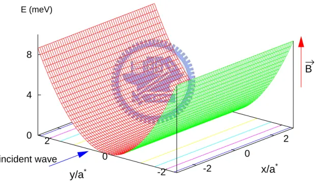
(23) ¨ CHAPTER 2. INTRODUCTION TO LANDAUER-BUTTIKER FORMULA AND OUR PHYSICAL MODEL We try to push our theoretical description of magnetoconduction in a narrow parabolic confining potential which is more realistic to the high magnetic field regime. We will investigate the transmission dip found at the threshold of subband for repulsive potential and the two transmission dips found for the incident energy lies below a subband threshold. And our approach can consider a general condition raging form low magnetic field to high magnetic field.. E (meV). 8. →. B 4. 0. 2. 2 0. 0. incident wave. y/a*. -2. -2. x/a*. Figure 2.1: The figure of our system. Our system of interest in this work is basically a quantum wire formed out of a 2DEG. The propagation direction o the wire is x whereas the confinement potential that define of quantum wire is given by Vc (y). Of particular interest is the effect of a magnetic field, pointing along z, on the transport characteristic in the presence of a transverse potential barrier.. 10.

(24) ¨ CHAPTER 2. INTRODUCTION TO LANDAUER-BUTTIKER FORMULA AND OUR PHYSICAL MODEL The confinement potential Vc (y) is chosen to be parabolic namely 1 Vc (y) = m∗ ωy2 y 2 , 2. (2.1). where m∗ is the effective mass of an electron in media and ωy is a potential parameter. The unperturbed Hamiltonian H0 of the electron in the constriction is given by ¸ · e ´2 1 ∗ 2 2 ~2 ³ −i∇ + A + m ωy y H0 = 2 c~ 2m∗. (2.2). where −e is the charge of the electron. And in this work we focus on the scattering effect due to an impurity, which the potential of impurity is Vd (x, y). The total Hamiltonian:. H=. e ~2 [−i∇ + A(r)]2 + Vc (y) + Vd (x, y) c~ 2m. (2.3). A(r) is the vector potential A(r) = −Byî → B(r) = ∇ × A = B kˆ. (2.4). Vc (y) is the confinement potential in the y-direction Vc (y) = 12 mωy2 y 2 H=. eB ˆ 2 1 ~2 y i] + mωy2 y 2 + Vd (x, y) [−i∇ − 2 c~ 2m. (2.5). And then we choose some units to obtain the dimensionless expression of Hamiltonian 1 ∗ ~2 kF2 ,ε = 2m∗ kF 2 ~c ε∗ ~kF ∗ ~kF2 ∗ ωc = ∗ , ωy = ∗ = 2 , B ∗ = kF2 . e ~ m m. a∗ = and hence. Here ωc = eB/m∗ c is the cyclotron frequency, and ωc = eB/m∗ c = (e/m∗ c) (~ckF2 /e) B = 11.

(25) ¨ CHAPTER 2. INTRODUCTION TO LANDAUER-BUTTIKER FORMULA AND OUR PHYSICAL MODEL (~kF2 /m∗ )B = ωc∗ B, and lB = (~c/eB)1/2 is the magnetic length. In our numerical examples, the nano-channel(NC) is taken to be that in a high mobility GaAs/Alx Ga1−x As with a typical electron density n ∼ 2.5 × 1011 cm−2 , and m∗ = 0.067 meV. Correspondingly, our choice of energy unit E ∗ = ~2 kF2 /(2m∗ ) = ˙ angular frequency unit 5, 933 meV, length unit a∗ = 1/kF = 9.7937 × 10−9 m = 97.937A, ωc∗ ~ = ωy∗ ~ = Ω∗ ~ = 2E ∗ = 11.866meV, and the magnetic field unit B ∗ = 6.863 Tesla. We also take ωy = 0.5 of which ωy ωy∗ ~ = 5.933 meV, such that the effective NC width ˙ In the following, in presenting the dependence of transmission is of the order of 102 A. on µ, it is more convenient to plot transmission(T) as a function of X instead, where X = µ/2ωy + 12 . The integral value of X is the number of propagating channels. The conservation of current condition is better represented by the function CSV (n) defined P as CSV (n) = log|1 − n0 (|tn0 n |2 + |rn0 n |2 )|, where n is the incident channel and n0 is the outgoing channel. We thus obtain the dimensionless Schrödinger equation ⇒ {−∇2 + Ω2 y 2 + 2iωc y. ∂ + Vd (x, y)}ψ(x, y) = Eψ(x, y) ∂x. (2.6). where Ω2 = ωc2 + ωy2 = ωy2 + B 2 In this work, we consider now electron scattering from an barrier potential of the form. Vd (x, y) = V0 Vs (y)δ(x − x0 ),. (2.7). where Vs (y) is an arbitrary function of the coordinate y, but we use it to be a uniform function of the transversal coordinate y and equal to 1 for simplify. x0 is the longitudinal position of the barrier, and the magnitude of V0 sets the magnitude of the barrier potential, which may be repulsive (V0 > 0) or attractive (V0 < 0). In Ch.3, we keep the scattering potential Vd (x, y) = V0 Vs (y)δ(x − x0 ) and Vs (y) is still an arbitrary function of the coordinate y in the analytical calculation, and set Vs (y) = 1 in the numerical process for a simpler system.. 12.

(26) ¨ CHAPTER 2. INTRODUCTION TO LANDAUER-BUTTIKER FORMULA AND OUR PHYSICAL MODEL Finally we can have the dimensionless Schrödinger equation of our physical model {−∇2 + Ω2 y 2 + 2iωc y. ∂ + V0 δ(x − x0 )}ψ(x, y) = Eψ(x, y) ∂x. 13. (2.8).

(27) Chapter 3 Mode-matching (MM) method In this chapter, we use the mode-matching approach to solve our physical model. After the formalism, we find that the eigen-function of the wire with magnetic field is not a orthogonal and complete basis set .The propagating mode with real wave vector has a center shift on y-direction and the evanescent mode become a highly oscillating complex function. We choose another orthogonal basis set φon (y) to expend the eigen-function φ± n (y, kn ) which is the better one in our three choices. We also find out a special normalization constant for the evanescent modes which are complex functions. The normalization constant of propagating modes and evanescent modes are different and the normalization constant of evanescent modes depend on the center shift αn .. 3.1. Formalism. We first solve the unperturbed Hamiltonian in this section and obtain the eigen-function of the confinement potential. In the previous Ch.2, we have obtained the dimensionless Schrödinger equation, Eq. (2.8) {−∇2 + Ω2 y 2 + 2iωc y. ∂ + Vd (x, y)}ψ(x, y) = Eψ(x, y) ∂x. 14. (3.1).

(28) CHAPTER 3. MODE-MATCHING (MM) METHOD Firstable, let’s solve the wavefunction of unperturbed Hamiltonian: {−∇2 + Ω2 y 2 + 2iωc y. ∂ }Ψ(x, y) = EΨ(x, y) ∂x. (3.2). Because the asymptotic form of wavefunction at x → ±∞ can be expanded as plane wave, we can assume the eigenfunction of this form Ψ(x, y) ∼ e±ikx φ± (y). (3.3). where k is a wavevector.. Substituting Eq. (3.3) the above wavefunction into Eq. (3.2), we obtain ¾ ωc k 2 ωc2 k 2 ∂2 2 2 − Ω (y ∓ 2 ) + 2 − k + E φ± (y) = 0 Ω Ω ∂y 2 ωc k let α = 2 , u± = y ∓ α, Ω. ½ ⇒. ⇒. ⇒. which the superscript ± of u denotes the right (left) going wave, ωy2 2 ωc2 k 2 2 2 − k + E = E − 2k and K = Ω Ω2 ¾ ½ 2 ∂ 2 − Ω2 u± + K 2 φ± (y) = 0 ∂u± 2 √ 0 let u± = Ωu± , ¾ ½ 2 K2 ∂ ±0 2 φ± (y) = 0 −u + 02 ± Ω ∂u. (3.4). (3.5). Based on the definition of Hermite function, we can obtain the discrete energy identity:. (2n + 1)Ω =. ωy2 2 ωc2 k 2 2 k − k + E = E − Ω2 Ω2. ±0. and φn (y) ∝ e−un. 2. /2. √ ± 2 0 u± −Ω 2 n H ( Ωun ) Hn (u± n n ) = e. 15. (3.6). (3.7).

(29) CHAPTER 3. MODE-MATCHING (MM) METHOD. In Eq. (3.6), the energy is quantized, and then we change our variables to have the quantized physical quantities labeled by the subband index n: ωc kn ± , u → u± n = y ∓ αn , 2 Ω √ 2 −Ωu± n /2 Hn ( Ωu± φ± (y) → φ± n) n (y, kn ) = Nn × e k → kn , α → αn =. We can write down the total wavefunction: 2 /2. ψn (x, y) = Nn e±ikn x e−Ω(y∓αn ). √ Hn ( Ω(y ∓ αn )). (3.8). ωy2 2 k = (2n + 1)Ω, Ω2 n ωc kn = y ∓ α n , αn = Ω2 p Ω E − (2n + 1)Ω, Ω2 = ωy2 + ωc2 . = ωy. εn = E − u± n kn. and φ± n (y, kn ) is the eigenfunction of this equation ½. ¾ ωc kn 2 ∂2 2 2 − Ω (y ∓ 2 ) + K φ± n (y, kn ) = 0 Ω ∂y 2. (3.9). which is a shifted harmonic oscillator of frequency Ω, The center of the transverse eigen2 function φ± n (y, kn ) is at y = ±ωc kn /Ω . Hence the larger the momentum ±~kn along. x-direction, the more the center of wave function is shifted, and φ± n (y, kn ) is not longer a complete set. The center shift of wavefunction may be real or pure imaginary because it depends on the momentum kn along x-direction.. 16.

(30) CHAPTER 3. MODE-MATCHING (MM) METHOD. 3.2. Normalization constant and evanescent mode. 2 The eigen-function φ± n (y, kn ) have a shift constant αn = ωc kn /Ω which have presented in. the previous chapter. The shift constant and the wave vector become a pure imaginary number for the evanescent modes, and the eigen-function become a complex function. We have to redefine the normalization constant for both propagating modes and evanescent modes, the normalization constant of propagation constant is similar to the case without magnetic field; the normalization constant of evanescent modes is different and be a more smaller number to confine the evanescent modes. And we also compare the normalization constant of propagating modes and evanescent modes and find out the relation between them. In this section, we will determine the normalization constant for both the wave vector s kn are real and pure imaginary of the eigen-function φ± n (y, kn ). We use Nn for the real. kn , and Nn for the pure imaginary one. We first write down the normalization identity, Z ± φ±∗ n (y, kn )φn (y, kn ) dy = 1.. and then we discuss the two case of real and pure imaginary wave vector kn ± 1) If kn is real: (φ±∗ n = φn ). Z ± φ± n (y, kn )φn (y, kn )dy = 1, Z ∞ √ 2 s2 Nn e−Ω(y∓αn ) Hn [ Ω(y ∓ αn )]dy = 1, −∞ √ let Ω(y ∓ αn ) = x± , Z Nns 2 ∞ −x±2 2 ± ± e Hn (x )dx = 1, ⇒ √ Ω −∞ Z √ 2 and e−x Hn2 (x)dx = 2n n! π,. µ ⇒. Nns. =. r ¶−1/2 π . 2 n! Ω n. 17. (3.10).

(31) CHAPTER 3. MODE-MATCHING (MM) METHOD. 2) If kn is pure imaginary: substituting Eq. (3.8) into the normalization identity, Eq. (3.10), we have. Z. √ √ Ω Ω 2 ∗ 2 e− 2 (y∓αn ) Hn [ Ω(y ∓ αn∗ )]e− 2 (y∓αn ) Hn [ Ω(y ∓ αn )]dy = 1 −∞ √ √ let x = Ωy, qn = Ωαn Z ∞ 1 dx 2 ∗ 2 1 2 Nn e− 2 (x∓qn ) − 2 (x∓qn ) Hn [x ∓ qn∗ ]Hn [x ∓ qn ] √ = 1 Ω −∞ √ Ω ±qn∗ − (±qn ) ∗ (±αn∗ − (±αn )) = where an = ±qn + (±qn ), bn = 2 2 −b2n Z ∞ e 2 e−x Hn [x − bn ]Hn [x + bn ]dx (3.11) Nn−2 = √ Ω −∞. Nn2. ⇒. ∞. Using the Eq. (A.78), we have: Z∞ 2. e−x Hm (x + a)Hn (x + b)dx −∞. √ m!n! π 2 a b = k!(m − k)!(n − k)! k=0 µ ¶µ ¶ M in[m,n] X √ n m+n−k m−k n−k n k! π 2 a b = k k k=0 M in[m,n]. X. m+n−k m−k n−k. (3.12). using Eq. (3.12) and Eq. (3.11), it is easy to obtain the normalization constant of the. 18.

(32) CHAPTER 3. MODE-MATCHING (MM) METHOD following form r Nn−2. = r. µ ¶µ ¶ n n π −b2 X 2n−k 2 n−k n 2 (−bn ) e k! Ω k k k=0 n. n!2 π −b2n X 2n−k 2 (−b2n )n−k e k! (n − k)!2 Ω k=0 µ ¶ n X (2ΩIm(αn )2 )k n s −2 ΩIm(αn )2 = Nn e k k! k=0. =. and bn. (3.13). √ √ Ω ±qn∗ − (±qn ) (±αn∗ − (±αn )) = ∓i ΩIm(αn ), = = 2 2. b2n = −ΩIm(αn )2 .. Im(αn )2 −Ω 2. Nn = Nns e. #−1/2 " n X (2ΩIm(αn )2 )k µn¶ k. k!. k=0. (3.14). Define the normalization constant factor Λn for the evanescent modes. Λn ≡. #−1/2 " n X (2ΩIm(αn )2 )k µn¶ k. k!. k=0. Ω. .. (3.15). 2. In the propagating modes and kn is real, e− 2 Im(αn ) Λn = 1 and Nn = Nns . In the Ω. 2. evanescent modes, e− 2 Im(αn ) Λn is smaller than 1 and Nn is smaller than Nns , ωy 2 √ In the case of zero magnetic field, φsn (y) reduce to φon (y) = Nno e− 2 y Hn ( ωy y), where q Nno = (2n n! ωπy )−1/2 . Correspondingly, we get √ Ω 2 φsn (y) = Nns e− 2 y Hn ( Ωy) φon (y) = Nno e−. ωy 2. y2. √ Hn ( ωy y). √ ± 2 u± Im(αn )2 − Ω −Ω s 2 n H ( 2 Ωun ) e Λ e (y, k ) = N φ± n n n n n. 19. (3.16) (3.17) (3.18).

(33) CHAPTER 3. MODE-MATCHING (MM) METHOD. 3.3. Mode-matching approach. In this section, we use the mode-matching approach to solve the problem with a δ-type impurity barrier. We write down the formalism in a general way for three kinds of basis set to expand the eigen-function φ± n (y, kn ). We consider an impurity or an external potential in a quantum wire, the system under investigation can be described by H = H0 + Vd (x, y), where. H0 = −∇2 + Ω2 y 2 + 2iωc y. ∂ ∂x. (3.19). is the unperturbed Hamiltonian, Vd (x, y) = V0 δ(x)Vs (y) which is the scattering potential. The incident wavefunction from left (L) lead is given by ψin (x, y, kl ) = eikl x φ+ l (y, kl ). (3.20). The corresponding scattering wavefunction is of the form  P + −ik 0 x −   rn0 l e n φn0 (y, kn0 )  ψ(x < x0 , y, kn ) = eikl x φ+ l (y, kl ) +    ψ(x > x0 , y, kn ) =. P n0. n0. ikn0 x + φn0 (y, kn0 ) t+ n0 l e. where 2. Ω. − 2 (y∓αn ) Hn φ± n (y, kn ) = Nn e. h√. i Ω(y ∓ αn ) .. ,. (3.21). (3.22). In addition, we can expand the wavefunction φ± n (y, kn ) into several sets of basis like √ √ y2 s −Ω s −Ω(y∓αn )2 /2 2 Ωy), and φon (y) = H ( e (y) = N Ω(y ∓ α )], φ (y, k ) = N e H [ φ± n n n n n n n n ωy 2 P ± √ (±)± , φ± Nno e− 2 y Hn ( ω y y). And the wavefunction φ± n (y, kn ) = n (y, kn ) = j φj (y)Cjn R P o P s (o)± (±)± (s)± (s)± ± = δjn , Cjn = dy φsj (y)φ± n (y, kn ), j φj (y)Cjn , where Cjn j φj (y)Cjn , or φn (y, kn ) = R (o)± and Cjn = dy φoj (y)φ± n (y, kn ) correspondingly. In mathematically, no matter what kind of complete set we used, the result should be the same. But according to the center shift of the propagating and evanescent modes, the results are different and we will discuss in. 20.

(34) CHAPTER 3. MODE-MATCHING (MM) METHOD the Sec. 3.5. (±,s,o). In order to simplify the formalism, we use χn. (y) to replace the functions φ± n (y, kn ),. φsn (y), and φon (y) correspondingly. X. φ± n (y, kn ) =. (±,s,o). χj. j. φ± n (y, kn ) =. or. (±,s,o)±. (y)Cjn X. ± χj (y)Cjn. (3.23) (3.24). j. And then we can rewrite Eq. (3.21) of the below form. ψ(x < x0 , y, kn ) =. X. eikl x χj (y)Cjl+ +. ψ(x > x0 , y, kn ) =. − + e−ikn0 x χj (y)Cjn 0 rn0 l. (3.25). n0 ,j. j. X. X. + + eikn0 x χj (y)Cjn 0 tn0 l. (3.26). n0 ,j. The Schrödinger equation in the presence of Vd (x, y) is given by ·. ¸ ∂ ∂2 ∂2 2 2 + Ω y + V0 δ(x − x0 )Vs (y) ψ(x, y) = ψ(x, y) − 2 − 2 + 2iωc y ∂x ∂y ∂x. (3.27). The scattering should satisfy two boundary conditions, one requirement is that ψ(x, y) has to be continuous at x = xi and the other one stems from integration of the Schrödinger equation across x = xi . The wavefunction is continuous at x = 0 :. ψ|0+ = ψ|0−. ⇒. X j. χj (y)Cjl+ +. X. − + χj (y)Cjn 0 rn0 l =. n0 ,j. (3.28) X n0 ,j. 21. + + χj (y)Cjn 0 tn0 l. (3.29).

(35) CHAPTER 3. MODE-MATCHING (MM) METHOD By integrating the Schrödinger equation through x = 0 , we get X. + + ikn0 χj (y)Cjn 0 t n0 l −. n0 ,j. X. ikl χj (y)Cjl+ +. X. − + ikn0 χj (y)Cjn 0 rn0 l −V0 Vs (y). + + χj (y)Cjn 0 t n0 l = 0. n0 ,j. n0 ,j. j. X. (3.30) Multiply these two boundary conditions Eq. (3.29) and Eq. (3.30) by χj 0 (y) and then integrate over y, we obtain Cj+0 l +. X. Cj−0 n0 rn0 l =. X. + ikn0 Cj+0 n0 t+ n0 l − ikl Cj 0 l +. X. ikn0 Cj−0 n0 rn+0 l − V0. X. + + fχ,j 0 j Cjn 0 tn0 l = 0.. (3.32). n0 ,j. n0. n0. (3.31). n0. n0. X. Cj+0 n0 t+ n0 l ,. where we use the below conditions. For χn (y) = φsi (y) or χo (y) = φoi (y), we have Z. ∞. dy −∞. (s,o) (s,o) ∗ (y)χi (y) χi. Z. ∞. = δi,j ;. (s,o) ∗. dy χi. −∞. (s,o). (y)Vs (y)χi. (s,o). (y) = fχ,ij .. (3.33). and for χn (y) = φ± n (y, kn ), we have Z. Z. ∞. dy Z−∞ ∞. ∗ ± χ± i (y)χi (y) (±) ∗. dy χi. −∞. ∞. =. (±)± ∗. dy φi. −∞ (±). (±)±. (y, kn )φj. (±). (y)Vs (y)χi (y) = fχ,ij .. (y, kn ). (3.34) (3.35). and we redefine the coefficient Z (±)± Cij. =. (±)± ∗. dy φi. (±)±. (y, kn )φj. 22. (y, kn ).. (3.36).

(36) CHAPTER 3. MODE-MATCHING (MM) METHOD In order to extend Eq. (3.31) and Eq. (3.32) to matrix form, we define that: . [t± mn ]j×l.      ≡     . . ± ]j×l [rmn. ··· .. .. t± 0n. t± m0 · · · .. .. t± mn .. .. t± j0. ···. t± jn. ± r00 .. .. ··· .. .. ± r0n .. .. .. ..      ± ≡  rm0 · · ·   ..  .  ± ··· rj0 . ± [Cmn ]j×l. t± 00. ± C00. .. .. ± rmn .. . ± rjn. ···. t± 0l. .  ..  .    ±  · · · tml   . . . ..  .   ± · · · tjl. (3.37). .. (3.38). j×l. ···. ± r0l .. .. .      ±  · · · rml   ..  ... .   ± · · · rjl. ± C0n. C0l±. ··· ···   .. .. .. ...  . . .   ± ± ± ≡  Cm0 · · · Cmn · · · Cml  .. ..  .. .. . . .  .  ± ± · · · Cjl± · · · Cjn Cj0. j×l.            . ;. (3.39). j×l. .  fχ,00 .. .. [fχ,mn ]j×l. ;. ··· .. ..      ≡  fχ,m0 · · ·   ..  .  fχ,j0 · · ·. 23. fχ,0n .. .. ···. fχ,0l .. .. fχ,mn · · · fχ,ml .. .. .. . . . fχ,jn. ···. fχ,jl.           . .. j×l. (3.40).

(37) CHAPTER 3. MODE-MATCHING (MM) METHOD And then we can write down Eq. (3.31) and Eq. (3.32) in matrix form + − + + [Cmn ]j 0 ×l + [Cmn ]j 0 ×n0 [rmn ]n0 ×l = [Cmn ]j 0 ×n0 [t+ mn ]n0 ×l. (3.41). + + [Cmn ]j 0 ×n0 [km δmn ]n0 ×n0 [t+ mn ]n0 ×l − [Cmn ]j 0 ×l [km δmn ]l×l + + − ]n0 ×l + iV0 [fχ,mn ]j 0 ×j [Cmn +[Cmn ]j×n0 [t+ ]j 0 ×n0 [km δmn ]n0 ×n0 [rmn mn ]n0 ×l = 0 (3.42). Let j 0 = j = n0 = l = Nc , all the matrices become square matrixes, where Nc is the total number of subband we used in the numerical calculation + − + + [Cmn ] + [Cmn ][rmn ] = [Cmn ][t+ mn ]. (3.43). + + − + + + [Cmn ][km δmn ][t+ mn ] − [Cmn ][km δmn ] + [Cmn ][km δmn ][rmn ] + iV0 [fχ,mn ][Cmn ][tmn ] = 0. (3.44). ± And then, it is trivial to get the coefficient of t± mn and rmn by the inverse.. . . ±  [tmn ]    ± [rmn ] 2Nc ×Nc −1  ∓ ± − [Cmn ] [Cmn ]   =   ∓ ± ± ] [km δmn ] ] [Cmn ] [km δmn ] + iV0 [fχ,mn ] [Cmn [Cmn. 2Nc ×2Nc. 1. 2. − 2 Ω(y∓αn ) Hn φ± n = Nn e. h√. (3.45) .   . ± ] [Cmn ± ] [km δmn ] [Cmn.   2Nc ×Nc. i Ω(y ∓ αn ) have a good physical meaning because it is the. eigenfunction in the wire in parabolic confinement with magnetic field, but not a complete h√ i 1 2 Ωy is set in this space, and cause some mathematic problems. φsn (y) = Nns e− 2 Ωy Hn the ordinary unshifted harmonic oscillator with confinement frequency Ω. We use this basis to be the projecting basis χn (y), this is a complete set rather than φ± n , and has the same oscillation frequency Ω. It has good character in calculation and better behavior in small magnetic, but still diverge in some cases we want to see. And then we use the ¤ £√ 1 2 eigenfunction φon (y) = Nno e− 2 ωy y Hn ω y y which is the eigenfunction in parabolical wire 24.

(38) CHAPTER 3. MODE-MATCHING (MM) METHOD without magnetic field. It is also a complete set, but stronger calculation the other basis, φsn (y) and φ± n (y). This is the best basis in these three eigenfunctions, some problem had be solved and good conservation in most case with not very strong magnetic field. In this section we choose φon (y) to be our projecting basis, but we still list all of the others calculation in appendix.. Z (o)± Cmn. dy φom (y)φ± n (y) s Ωαn 2 1 1 2 2m!n! (ωy Ω)1/4 e 2 η( η ) − 2 ΩRe[αn ] Λn = η ¸ · √ i h √ 2ωy Ωαn ¯ m−p ± 2Ωωy αn H ¯ m n ∓ H η XX n−q η × 2q 2p p=0 q=0  Min[p,q]−1  2  P   ) , m, n are both odd. ) fr3 ( q−2s−1 fr1 (2s + 1) fr2 ( p−2s−1  2 2  s  P (3.46) × (Min[p,q])/2 ) , m, n are both even. ) fr3 ( q−2s fr1 (2s) fr2 ( p−2s  2 2   s     0 , m + n is odd.. =. ¯ n (x) ≡ Hn (x) , η = ωy + Ω, αn = ωc kn where H Ω2 2n n!. and. p 8 ωy Ω n ) /n!, fr1 (n) = ( η 3ωy − Ω n ) /n!, fr2 (n) = ( η 3Ω − ωy n ) /n!. fr3 (n) = ( η. 25. (3.47). (3.48) (3.49) (3.50).

(39) CHAPTER 3. MODE-MATCHING (MM) METHOD. Z o fχ,mn. ∞. = −∞. r =. 3.4. φoi ∗ (y)Vs (y)φoi (y)dy r. Min[m,n] κ X 2 ( ωyβ+β )m−κ ( ωyβ+β )n−κ ωy −a2 Hm+n−κ [a] (3.51) e (n − κ)! (m − κ)! κ! ωy + β κ=0 s βωy y0 . (3.52) where a = ωy + β. m!n! 2m 2n. Current density and conservation condition. The current density in a system with magnetic field is different from the case without magnetic field. In this section, we use the Hamiltonian of our system and the continuous equation to get the form of current density in a magnetic field. And we also know that the net current is contributed from the propagating modes and wave vector kn is real; the current density in the evanescent mode is not zero but does not contribute to the total net current. We first write down our Hamiltonian and the continuous equation ∂ ∂2 ∂2 ∂ = − 2 − 2 + 2iωc y ∂x ∂y ∂x ∂x 2 2 ∂ ∂ ∂ = − 2 − 2 − 2iωc y ∂x ∂y ∂x. H = −∇2 + 2iωc y H∗. ∂ ρ = i(H ∗ ψ ∗ H − ψ ∗ Hψ) = −∇ · j ∂t. 2 ∂2 ∗ ∗ ∂ ψ∗ ψ )ψ + ψ 2 2 ∂x ∂x ∂ ∂ ∗ ∂ ∂ ∗ ∂ ∂ ∂ ∗ ψ·ψ ψ) − (ψ ψ+ ψ = − ( ψ · ψ) + ∂x ∂x ∂x ∂x ∂x ∂x ∂x ∂ ∗ ∂ ∂ ψ · ψ} {ψ ∗ ψ − = ∂x ∂x ∂x. (−. 26. (3.53) (3.54). (3.55).

(40) CHAPTER 3. MODE-MATCHING (MM) METHOD ∂ ∂ ∗ ψ )ψ − ψ ∗ (2iωc y )ψ ∂x ∂x ∂ ∗ = −2iωc y (ψ ψ) ∂x ∂ (−2iωc yψ ∗ ψ) = ∂x. (−2iωc y. ⇒. ∂ ∗ ∂ 1 ∂ ∂ ∗ ∂ −1 ∂ ∂ ψ · ψ} {ψ ∗ ψ − ψ · ψ − 2iωc yψ ∗ ψ} − {ψ ∗ ψ − ρ = ∂y ∂y i ∂y ∂x ∂x i ∂x ∂t ∂ 1 ∂ ∂ −1 ∂ (3.56) {ψ ∗ ψ − c.c.} − iωc y)ψ − c.c.} − {ψ ∗ ( = ∂x i ∂y ∂x i ∂x. and then we can define the current density along x- and y-direction ∂ ∗ ∂ 1 ψ · ψ − 2iωc yψ ∗ ψ} jx = {ψ ∗ ψ − ∂x ∂x i. (3.57). ∂ ∗ ∂ 1 ψ · ψ} jy = {ψ ∗ ψ − ∂y ∂y i. (3.58). The third term of Eq. (3.57), −2iωc yψ ∗ ψ, is caused from the applied magnetic field and the current density on x-direction is y-dependent in the coordinates.. 3.4.1. Current conservation on the longitudinal direction. In this subsection, we investigate the conservation condition on the longitudinal direction, the applied magnetic field introduce a factor depend on the magnetic field to the conservation condition. But the form of conservation condition is same as the one without magnetic field. The total wavefunctions on the left and right side of the scattering potential are given by  P −ik 0 x −   e n φn0 (y)rn0 l  ψL = eikl x φ+ l (y) + n0.  +∗   ψL∗ = e−ikl x φl (y) +. P n0. ∗ x ikn 0. e. ∗. ∗ φ− n0 (y)rn0 l. 27. and.  P ik 0 x −   e n φn0 (y)tn0 l  ψR = n0.    ψR∗ =. P n0. ∗. ∗. ∗ e−ikn0 x φ− n0 (y)tn0 l. (3.59).

(41) CHAPTER 3. MODE-MATCHING (MM) METHOD where l is the incident state and kl is a real number. Substitute Eqs.(3.59) in to Eq. (3.57) and obtain ∗. + kl φ+ l (y)φl (y) −. +. X. X n0. ∗ ∗ + ∗ kl ei(kn0 +kl )x φ− n0 (y)φl (y)rn0 l. n0 ∗. + +kl φ+ l (y)φl (y) +. −. X. X. ∗. + −2ωc y{φ+ l (y)φl (y) +. +. −. X. ∗. ∗. − ∗ kn00 ei(kn0 −kn00 )x φ− n0 (y)φn00 (y)rn0 l rn0 l. n0 ,n00 ∗. − kl e−i(kn0 +kl )x φ+ l (y)φn0 (y)rn0 l. n0 ∗ + ∗ kn∗ 0 ei(kn0 +kl )x φ− n0 (y)φl (y)rn0 l. n0. X. ∗. − kn0 e−i(kn0 +kl )x φ+ l (y)φn0 (y)rn0 l. X. −. X. ∗. ∗. − ∗ kn∗ 00 ei(kn0 +kn00 )x φ− n0 (y)φn00 (y)rn0 l rn0 l. n0 ,n00 ∗. − kn0 e−i(kn0 +kl )x φ+ l (y)φn0 (y)rn0 l. n0 ∗. + ∗ ei(kn0 +kl )x φ− n0 (y)φl (y)rn0 l +. X. ∗. − ∗ ei(kn0 −kn00 )x φ− n0 (y)φn00 (y)rn0 l rn0 l. (3.60). n0 ,n00. n0. in the left side of impurity barrier, and X. ∗. ∗. + ∗ kn00 e−i(kn0 −kn00 )x φ+ n0 (y)φn00 (y)tn0 l tn00 l +. n0 ,n00. −2ωc y. X. X. ∗. ∗. + ∗ kn0 e−i(kn0 −kn00 )x φ+ n0 (y)φn00 (y)tn0 l tn00 l. n0 ,n00 ∗ −k −i(kn 0 n00 )x. e. ∗ + ∗ φ+ n0 (y)φn00 (y)tn0 l tn00 l. (3.61). n0 ,n00. in the right side. And then integrate these two equations, Eq. (3.60) and Eq. (3.61), over x from −∞ to ∞, and we find that some terms with imaginary kn is vanish in this integration. The left side should equal to the right side, and we have ∗. + kl φ+ l (y)φl (y) −. =. X n0. X. ( ∗. − 2 kn0 φ− n0 (y)φn0 (y)|rn0 l | − ωc y. n0 ∗. + 2 kn0 φ+ n0 (y)φn0 (y)|tn0 l | − ωc y. X. ∗. + φ+ l (y)φl (y) +. X. ) ∗. − 2 φ− n0 (y)φn0 (y)|rn0 l |. n0 ∗. + 2 φ+ n0 (y)φn0 (y)|tn0 l |. n0. where the summation sum over all propagation modes.. 28. (3.62).

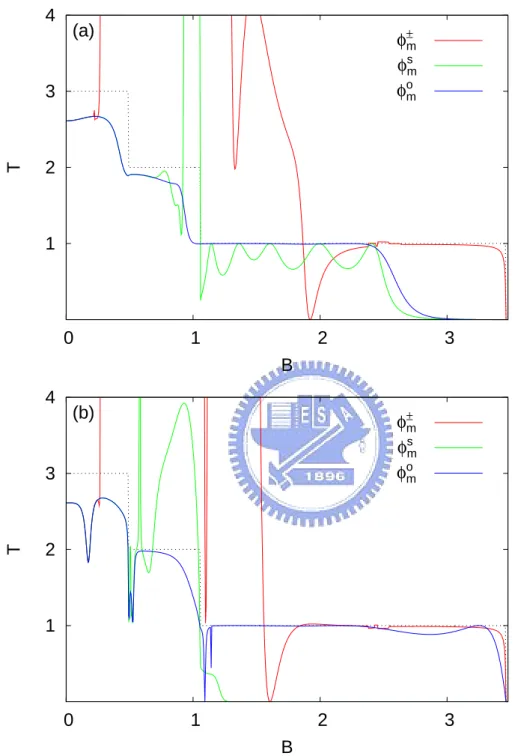
(42) CHAPTER 3. MODE-MATCHING (MM) METHOD And then integrating over y, we also have the following two equation Z ∗. ± φ± n (y, kn ) φn (y, kn )dy = 1, which is the normalization condition.. Z ∗. ± yφ± n (y, kn ) φn (y, kn )dy = ±Re[αn ] =. ±ωc Re[kn ] Ω2. (3.63). where kn is real and φ± n (y, kn ) a is real function and a orthogonal set. Finally we have the conservation equation in the x-direction:. ⇒. ) ( X X ωc2 kn0 |rn0 l |2 − kl = 0 kn0 |tn0 l |2 + (1 − 2 ) Ω n0 n0. (3.64). where summation sum over the propagating modes and the wave vector must be real.. 3.5. Numerical results. In the Fig. 3.1, we plot the results of the transmission as a function of applied magnetic field to compare the numerical results of the three basis sets. There are three curves s in both figures, which are the results using the different basis in order, φ± n (y, kn ), φn (y). and φon (y). Except changing the basis, we fix Nc = 17, incident energy is at 7ωy E ∗ , and V0 = 1.0E ∗ in (a) and V0 = −1.0E ∗ in (b). The block dashed line is the transmission without any scattering potential in the wire. The three curves in the both figures are the results by using the different basis in order. s It is easily to see that the results (curves) of φ± n (y, kn ) and φn (y) exceed the permitted. range (The transmission must below the black dashed line in the figures). And the third curve of projecting to the basis φon (y) is more reasonable, this curve all below the black dashed line. Although the three curves look quite different, but all of them lie together on the same line in the range of low magnetic filed (below B = 0.2). This result show that the calculation in this chapter works in the low magnetic regime no matter what basis we used, and the selection of basis effect a lots in the high magnetic regime. 29.

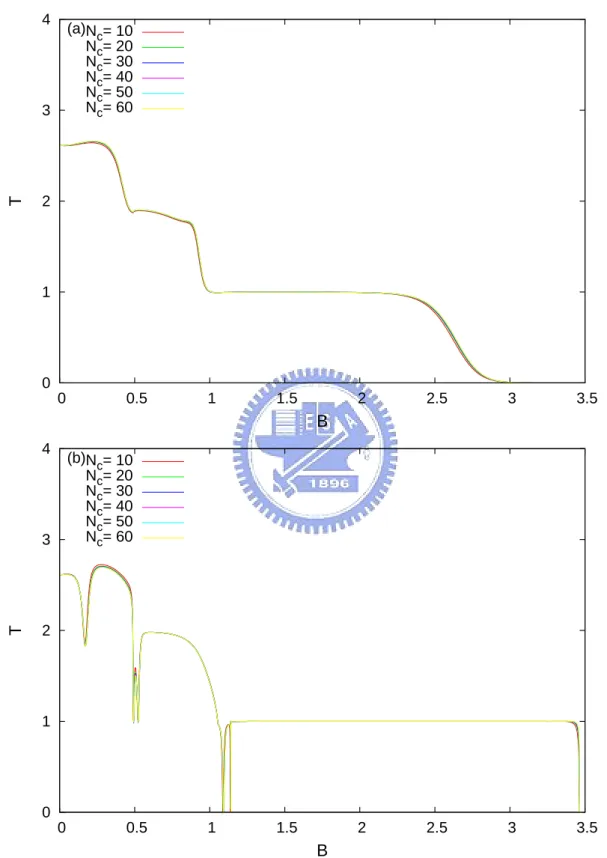
(43) CHAPTER 3. MODE-MATCHING (MM) METHOD. 4. (a). φ±m φsm φom. T. 3. 2. 1. 0. 1. 2. 3. B 4. (b). φ±m φsm φom. T. 3. 2. 1. 0. 1. 2. 3. B Figure 3.1: Compare the numerical results of three basis sets. The red line is the result s projected to φ± m (y, km ); the green one is projected to φm (y); and the blue one is projected o to φm (y). The strength of the impurity barrier is repulsive with 1.0E ∗ in (a) and attractive with −1.0E ∗ in (b). Base on this comparison, we finally choose the basis set φon (y) to be our projecting basis in this work. In the Fig. 3.2, we fix the incident energy at 7ωy E ∗ and plot the transmission as a 30.

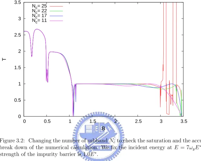
(44) CHAPTER 3. MODE-MATCHING (MM) METHOD. 3.5. Nc= 25 Nc= 22 Nc= 17 Nc= 11. 3 2.5. T. 2 1.5 1 0.5 0 0. 0.5. 1. 1.5. 2. 2.5. 3. 3.5. B. Figure 3.2: Changing the number of subband Nc to check the saturation and the accuracy break down of the numerical calculation. We fix the incident energy at E = 7ωy E ∗ , the strength of the impurity barrier is 1.0E ∗ . function of B for various Nc to check the saturation and accuracy break down of numerical calculation. The strength of the attractive barrier in the wire is V0 = −1.0E ∗ . Except the regime of high magnetic field, the more numbers of subbands we used in the calculation, the curves saturate form low magnetic field to more high magnetic field. But as long as we use too many of numbers of subbands, like 22 and 25 in the Fig. 3.2, the curves diverge when the magnetic field larger than 3.3B ∗ and 3.0B ∗ , the more numbers of subbands we used in the calculation, the lower amplitude of magnetic field the curves diverge. This divergence is due to the accuracy in the computation is not enough. When the magnetic field is high, the structure of the matrix used to calculate the transmission and reflection will be difficult to find out its the inverse. It is easily diverged and need more accuracy to have the correct solution with less error. And the more elements of the matrix, the accuracy error will be enlarged. In the programs, we have already use the higher precision, quad-precision, than double precision to calculate the inverse of the matrixes, but in the 31.

(45) CHAPTER 3. MODE-MATCHING (MM) METHOD case of high magnetic field, it is not enough and still diverged, just like the curves in Fig. 3.2. This problem about the accuracy is the main problem if we want to have the saturate result in higher magnetic field, and we will discuss with this later. In the Fig. 3.3, we plot the transmission as a function of incident energy for various numbers of subband form 26 to 30 to check the saturation the curves. The applied magnetic field is 1.0B ∗ and the strength of impurity barrier is repulsive with 1.0E ∗ in (a) and attractive with −1.0E ∗ in (b). As the increasing of the numbers of subbands, the curves saturate form the lower incident energy to higher energy but slowly. In the Fig. 3.3, B = 1.0B ∗ , we find that the curves saturate below X = 4 when we use 30 subbands. In the range of X > 4, the curves is not really saturate as we magnify the figures. Consider 30 subbands as the most total number of subband we can used in the calculation remaining accuracy for the case of B = 1.0B ∗ . When the numbers of subbands is more than 30, in the case of B = 1.0B ∗ , the curve will diverge. And in the case of B > 1.0B ∗ , the curve diverge before saturate even if X < 3.0; on the contrary, the curves saturate and using fewer numbers of subbands than 30 if the amplitude of magnetic field is smaller than B = 1.0B ∗ .. 3.6. Summary and discussions. In this chapter, we use the mode-matching approach to solve the magnetoconduction in the wire. The transverse eigen-function in the wire with magnetic field is written as 2 ± φ± n (y, kn ), and the center of the eigen-function φn (y, kn ) is at y = ±ωc kn /Ω . As the wave. vector kn is real, the center shift along the y-direction, the larger of ωc kn , the more the center shift. As the wave vector kn is pure imaginary, the center of φ± n (y, kn ) back to the center of the y-direction and become a complex function. There are two reason why we can not expand the eigen-function φ± n (y, kn ) well. One is according to the center shift of the eigen-function φ± n (y, kn ), it is quite different to expand the eigen-function which has two kind of shift. And another is that the eigen-function φ± n (y, kn ) is not an orthogonal. 32.

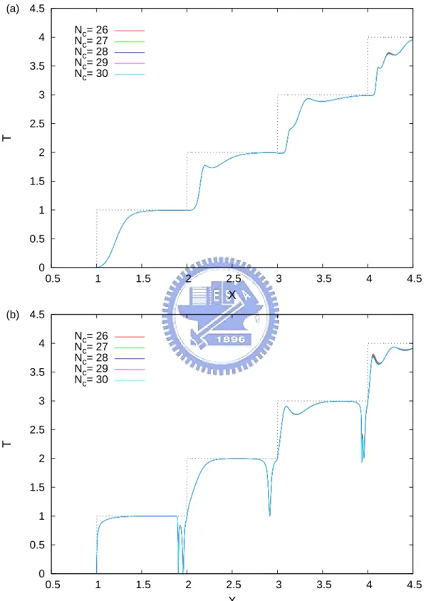
(46) CHAPTER 3. MODE-MATCHING (MM) METHOD. (a) 4.5 Nc= 26 Nc= 27 Nc= 28 Nc= 29 Nc= 30. 4 3.5 3. T. 2.5 2 1.5 1 0.5 0 0.5. 1. 1.5. 2. 2.5. 3. 3.5. 4. 4.5. 3. 3.5. 4. 4.5. X (b) 4.5 Nc= 26 Nc= 27 Nc= 28 Nc= 29 Nc= 30. 4 3.5 3. T. 2.5 2 1.5 1 0.5 0 0.5. 1. 1.5. 2. 2.5. X. Figure 3.3: The saturation of transmission versus Nc from 26 to 30 for B = 1.0 and the strength of impurity barrier is repulsive with 1.0E ∗ in (a) and attractive with −1.0E ∗ in (b).. 33.

(47) CHAPTER 3. MODE-MATCHING (MM) METHOD basis and incomplete set, we have to expand the eigen-function to another basis which is orthonormal. And that is why the transmission and conservation are not reasonable as we project the eigen-function to itself. There are two choices to expand the eigen-function, one is φsn (y) and the other is φon (y). φsn (y) is the eigen-function of a harmonic oscillation which the confinement is Ω2 y 2 on the y-direction. This kind of confinement, Ω2 y 2 , depend on the strength of the magnetic field and more confined in the large magnetic field regime than the original confinement, ωy2 y 2 . This eigen-function φsn (y) is more confined to the center more localized in the ydirection. And it may not cover the edge of the wire in a higher magnetic field where the edge state had generated. And then, the basis φon (y), which is the eigen-function in the wire without magnetic field. The covered range of this eigen-function φon (y) is more extensive in the y-direction then the eigen-function φsn (y), and match to the original wire which have the real edge state. And then we back to discuss the real eigen-function φ± n (y, kn ) in the wire. The character of this eigen-function is very different as the wave vector is real or pure imaginary. The center of the eigen-function shift and concentrate to the edge as the wave vector is real and the large kinetic energy and the magnetic field, the more shift. According to this phenomenon, it is better to choose the eigen-function φon (y) to be the projecting basis. But in the case of the wave vector is pure imaginary, the eigen-function become evanescent mode does not have the center shift and back to the center of the y-direction. Because the wavefunction is back to the center, it is better to use the eigen-function φsn (y) to expand the evanescent modes in the center of y-direction, the eigen-function φsn (y) is also more confined to the center. The most problem is what character is more important in the higher strength of magnetic field, the difference is not very much in the low magnetic field. And find out the balance of the expansion between wave vector is real and pure imaginary(propagating modes and evanescent modes). And then we find that the eigen-function φon (y) is more balanced to expand both propagating modes and evanescent modes, and we use this basis 34.

(48) CHAPTER 3. MODE-MATCHING (MM) METHOD φon (y) to expand the eigen-function φ± n (y, kn ). In the classical-like picture, the wavefunction shift and concentrate on the edge of the incident energy level when we apply a large magnetic field, and become the edgestate. This phenomenon of edge states is more important than the evanescent modes in the center of y-direction and need to be describe well. And that is the reason why eigen-function φon (y) is better than φsn (y). And we also care about the divergence of the inverse of the matrixes, and we spend lots of time to improve the accuracy of the calculation in program. And Finally we change most of codes of the programs and the subroutine which solve the inverse of a matrix to quad-precision, but already touch the limit of the numerical calculation. According to this situation, we develop another method to solve this system, the approach of partial Fourier transformation of Lippmann-Schwinger equation, and we will illustrate in next chapter.. 35.

(49) Chapter 4 An approach of partial Fourier transformation of the Lippmann-Schwinger (PFTLS) equation In CH.3, the numerical results can not saturate in the high magnetic field regime and diverge with the numerical accuracy when we use more numbers of subband in calculation. We think that is because the eigen-function φ± n (y, kn ) is not an orthogonal basis set and the shift properties of the propagating modes and the evanescent modes are different, it is hard to find a basis set which can describe the propagating modes and evanescent modes well at the same time. In the reference [66], the author use a Fourier transformation on xdirection of the Schrödinger equation, and the problem can be technically simplified when turn to the mixed, momentum-coordinate representation of the wavefunction. We will use a similar technic to solve our problem. Due to this technic, partial Fourier transformation, the evanescent modes are not a complex function and the basis set of φ± n (y, k) (where k is the integrating variable of Fourier transformation) become a orthogonal set. This method can avoid the complex evanescent modes we worried about in the previous chapter, and 36.