半導體雙廠區產能相互支援的途程規劃

國 立 交 通 大 學

工 業 工 程 與 管 理 學 系

碩士論文

半導體雙廠區產能相互支援的途程規劃

Route Planning for Two Wafer Fabs with Capacity

Sharing Mechanisms

研究生：陳振富

指導教授：巫木誠 博士

半導體雙廠區產能相互支援的途程規劃

Route Planning for Two Wafer Fabs with Capacity Sharing

Mechanisms

研究生：陳振富

Student：Chen-Fu Chen

指導教授：巫木誠 博士

Advisor：Dr. Muh-Cherng Wu

國立交通大學

工業工程與管理學系

碩士論文

A Thesis

Submitted to Department of Industrial Engineering and Management

College of Management

National Chiao Tung University

In Partial Fulfillment of the Requirements

For the Degree of Master of Science

In

Industrial Engineering

June 2007

Hsin-Chu, Taiwan, Republic of China

半導體雙廠區產能相互支援的途程規劃

研究生：陳振富 指導教授：巫木誠 博士

國立交通大學工業工程與管理研究所

中文摘要

半導體產業是資本密集的產業。設備的成本非常昂貴。為了迅速對市場需求 的熱烈作回應，一般半導體公司通常在擴大產能能力上採取一個雙廠區的策略。 本篇論文針對雙廠區的途程規劃問題提出一種方法來求解此問題。途程規劃問題 可以包含兩部份：途程的切割點決策以及途程的生產比例決策，其目標是在一目 標生產週期時間下產出最大化。本研究利用 LP-GA 的方法來求解此問題。我們 首先利用線性規劃模組來決定途程切割點，然後用基因演算法來求得各途程的生 產比例解。結果顯示 LP-GA 方法明顯比其他方法好。 關鍵字：雙廠區、跨廠、途程規劃、產出、產能支援

Route Planning for Two Wafer Fabs with Capacity Sharing

Mechanisms

Student：Ting-Uao

Hung

Advisor：Dr. Muh-Cherng Wu

Department of Industrial Engineering and Management

National Chiao Tung University

Abstract

Semiconductor manufacturing is a capitally intensive industry. The cost of equipment is very expensive. In order to quickly respond to market demand booming, a semiconductor company usually adopts a dual-fab strategy in expanding capacity. This paper presents an approach to solve the route planning problem for a semiconductor dual-fab. The route planning problem involves two decisions—determining the cutoff point and route ratio for each product—in order to maximize the throughput subject a cycle time constraint. An LP-GA method is proposed to solve the route planning problem. We first use the LP module to make the cutoff point decisions, and proceed to use the GA module for making the decision of route ratio. Results show that the LP-GA method significantly outperforms the other methods.

誌 謝

本論文得以順利完成，最先要感謝的是巫木誠教授。在巫木誠教授辛苦的諄 諄教導下，在學術的研究上獲益良多，在人生的處事上也有很大的啟示，學習如 何有紀律、有系統的管理自己的日常生活，了解必須要將自己的本分完成之重要 性，這些方法的教導將使學生終身受益無窮。同時也感謝許錫美教授、彭德保教 授和洪一薰老師在論文口試時，所給予的寶貴意見與指導，讓本論文更臻完備。 在碩士的兩年中，特別感謝幫忙完成本論文的施昌甫學長，以及半導體製造 管理中心所提供的相關軟體。其次要感謝博士班學長蘇泰盛、林姍慧學姊，同門 的傅進銘、李忠霖、施富騰、呂光棓與學弟妹們，陪我度過撰寫論文的這段日子， 互相討論，互相加油打氣，使我的碩士生活更充實且快樂，以及陳詠進、顏豪君、 吳政翰學長們對我的幫助，使我的研究生活更加充實。 感謝我最親愛的家人，在論文撰寫期間給我無數的關愛與幫助。特別是我的 父母親陳明瑞先生與簡月嬌女士，感謝你們多年來的辛勞與關懷，對我總是無怨 無悔的付出，對於你們的感謝，實非筆墨可以形容，還有我兩個弟弟對我的關懷， 最後謹以此論文獻給我最敬愛的家人、師長與朋友。 陳振富 于 新竹交大 2007/7/1

Contents

Chinese Abstract ... I EnglishAbstract... II Acknowledgement ...III Contents ...IV List of Tables... V List of Figures ...VI

Chapter 1 Introduction ...1

Chapter 2 Relevant Literature...3

Chapter 3 Problem Statement ...5

Chapter 4 Solution Framework ...7

Chapter 5 Module 1－P Model and Search Algorithm...9

5.1 LP Model...10

5.2 Binary Search Algorithm ... 11

Chapter 6 Module 2—Queueing and GA ...13

6.1 Queueing Network ...13

6.2 Genetic Algorithm...14

Chapter 7 Experiments...17

7.1. Benchmarks and Data ...17

7.2 Performance Comparison...17

Chapter 8 Conclusion...21

List of Tables

Table 1: Cutoff points obtained by the LP program...18 Table 2: Comparison of mean cycle time ...19 Table 3: Comparison of throughput ...19

List of Figures

Fig 1 Solution Framework ...7

Fig 2 Process of the cutoff point ... 11

Fig 3 Relationship between throughput and cycle time for product mix RA...20

Chapter 1 Introduction

Semiconductor manufacturing is a capitally intensive industry. The cost of equipment is very expensive. A typical 12 inch wafer fab costs about two billion dollars; over 80% of the expense is for equipment. The lead time for the acquisition of equipment is quite long, ranging from 3 to 9 months. In contrast, building factory space is relatively low in expense but with a much longer lead time—taking about one to two years.

In order to quickly respond to market demand booming, a semiconductor company usually adopts a dual-fab strategy in expanding capacity. That is, a large-scale factory space which could accommodate two fabs is established in advance. Then, equipments for the two fabs are gradually moved into the space according to the market demand trace over time. Finally, the semiconductor company has two fabs, which are in operation and close to each other in location.

With such a dual-fab configuration, a relatively easy way to manage a fab is manufacturing each wafer job within a particular fab. That is, each fab is run separately, without any mutual support in capacity. Such a separate-operation paradigm would usually lead to the underutilization of equipment. To remedy the underutilization issue, a cross-fab production paradigm is proposed. That is, a wafer job is partly manufactured in one fab and partly manufactured in the other fab.

This cross-fab production paradigm yields a route planning problem—how to appropriately assign the operations of a wafer job to each of the two fabs. Only a few studies on such a route planning problem have been published. Toba et al. (2005) addressed the route planning problem in a real-time manner. Whenever an operation of a job is completed, a decision—which fab to manufacture the next operation—must be immediately made. Wu and Chang (2006) investigated the route planning problem

in a short-term or weekly manner. The two fabs exchange capacity weekly to maximize the total throughput.

Though having established significant milestones, these two prior studies have some limitations due to make an implicit assumption. They both assumed that the transportation times within a fab or among fabs are a constant. This implies that the transportation capacity is infinite, and the proposed capacity planning engine may yield too much transportation. This may lead to traffic jam and as a result may lower the throughput and lengthen the cycle time.

In semiconductor manufacturing, the wafer size has steadily increased over time. In an up-to-date fab (12 inch wafer fab), wafer jobs must be transported by automatic vehicles because a wafer job weighs about 30 Kg and cannot be handled manually. This may yield a traffic jam problem because the transportation capacity is limited. Our interview with practitioners indicates that the traffic jam symptom would occur, in particular for a dual-fab layout. Therefore, transportation capacity has to be considered in the route planning problem for an up-to-date fab.

This research investigates the route planning problem for a dual-fab layout and is unique in two-fold. First, we assume that the transportation capacity is finite and the transportation times would vary. Second, the route planning decision is made based on a relatively longer time horizon—for example, one or several months. This research—focusing on longer time horizon complements prior studies which focused on either short-term or immediate decisions on route planning.

The remainder of this paper is organized as follows. Section 2 describes literature relevant to this research. Section 3 presents the route planning problem in detail. Section 4 described the proposed solution method. Numerical experiments are discussed in Section 5 and concluding remarks are in the last section.

Chapter 2 Relevant Literature

Given a customer demand, there may exists more than one manufacturing sites to fulfill the demand. A decision problem is how to allocate the demand to each manufacturing site. This capacity allocation problem can be addressed either in product level or in operation level. For the problem in the product level, each site is designated to manufacture a set of products. This implies that a product should be completely manufactured within a single site—cross-site production is prohibited. While in the operation level, each site is designated to manufacture a group of operations. Then, the operations for manufacturing a product could be distributed among different sites—cross-site production is allowed. This leads to the need for studying the route-planning problem among different sites.

For the capacity allocation problem—without cross-site routes, Wu et al. (2005) have given a comprehensive survey. The multiple manufacturing sites may be governed by a single company ( Frederix 2001) or by different companies ( Rupp ＆ Ristic 2000）, ( Karabuk ＆ Wu 2003), ( Lee et al. 2006). Linear programming (LP) models are typically formulated to solve the problems ( Manmohan 2005). To address the interactions among manufacturing sites, Game theory was proposed to enhance the LP models ( Wu et al. 2005).

For the capacity allocation problem—with cross-site routes, most studies were addressed in the context of group technology (GT). That is, each site is a manufacturing cell and multiple cells form a factory. Cross-cell production for manufacturing a product is permitted. However, each product is preferably manufactured within a particular cell and cross-cell production should be minimized.

Most prior studies allocated the capacity demand to cells through solving a cell formation problem ( Lee ＆ Abhary 1997), ( Defersha ＆ Chen 2006), ( Kim et al.

2005), ( Vin et al. 2005), ( Nsakanda et al. 2006). That is, in order to minimize the number of cross-cell transportations, they have to answer how many cells should be formed and how each cell should be equipped. After the cell formation problem is solved, each product is assigned to a particular cell for handling most of its operations. The remaining operations, much fewer in number, are handled by other cells. A GT cell is designed only for manufacturing a group of products, and by nature is limited in functional capacity. Therefore, cross-cell routes are unavoidably demanded in GT in order to provide a comprehensive functional spectrum.

However, in the route-planning problem we address, each of the two fabs is assumed to be functionally comprehensive. That is, a product can be completely manufactured in either one of the two fabs. The purpose of cross-fab production is to increase the total throughput of the two fabs, and the rationale is explained below.

In practice, a semiconductor fab is equipped to fulfill a particular product mix—the demand forecast at the time of purchasing equipment. However, the demand of product mix may change over time. Therefore, a fab may be underutilized due to the significant change of assigned product mix. In addition, the two fabs, even both functionally comprehensive, may differ in number for each type of machines. This implies that their originally designed product mixes may also differ. Cross-fab production therefore is needed to increase the total throughput of the two fabs.

Chapter 3 Problem Statement

This section aims to describe the dual-fab route planning problem more precisely. We first present the assumptions that confine the context of the route planning problem; and then proceed to introduce the decision variables, objective function and constraints of the problem. In explaining the assumptions, the two fabs are respectively called Fabs A and B.

Assumption 1: Each fab is functional comprehensive. Each of the two

semiconductor fabs is functionally comprehensive. That is, each fab is so comprehensively equipped that it can handle the manufacture of each product by itself, without the functional support of the other fab.

Assumption 2: A product has four possible routes. To implement

cross-production, the manufacturing route of each product is cut into two parts, where the route’s break point is called a cut-off point. The two parts are manufactured in different fabs, and yield two possible routes for cross-production. One, represented by

β

α→ , denotes that the first part of the route is manufactured at Fab_A and the

second part is at Fab_B. The other one, represented by β →α , denotes

manufacturing at Fab_B and then at Fab_A. Since each fab is functionally

comprehensive, the manufacturing of a product thus has four possible routes, α, β,

β

α→ , β → , where α α and β denotes the routes in a single fab.

Assumption 3: The transportation path between any two workstations/buffers is unique, rather than multiple. In each fab, a transportation system for moving wafer

jobs has been established. Theoretically, there may exist multiple paths in transporting from a workstation to another; however, to reduce the complexity of traffic control, we predefine a fixed path for such a transport.

cutoff point and the ratios of its four possible routes (simply called route ratios). Let

the cutoff point and route ratios of product i be represented by (π_i, Ri). For n products

i

to produce—with a given product mix, the route planning problem is to determine (π ,

Ri) for each product in order to maximize the total throughput of the two fabs, subject

the dual-fab route planning problem is shown

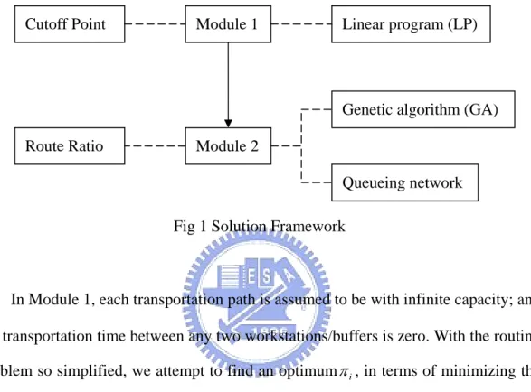
Fig 1 Solution Framework

uf

Chapter 4 Solution Framework

A framework proposed for solving in Fig. 1, which involves two modules.

In Module 1, each transportation path is assumed to be with infinite capacity; and the transportation time between any two workstations/b fers is zero. With the routing

problem so simplified, we attempt to find an optimumπ_i, in terms of minimizing the

number inter-fab transportations. The problem is solved by an iterative use of a linear

program (LP) model. For a particularπ_i, the LP model aims to compute its mi mum

number of inter-fab transportations, which is regarded as the performance of _i

ni

π . We

then develop a binary search algorithm to identify an optimum π_i as the ultimate

decision for cutoff point.

In Module 2—with the obtained π_i taken as parameters, we deal only with the

decision variables Ri. In this module, each transportation path is taken as a tool with

limited capacity. The transportation time required for passing a path can be varied, depending upon the traffic flow intensity. The higher the traffic intensity, the longer is the cycle time.

Module 1

Module 2

Linear program (LP)

Genetic algorithm (GA) Cutoff Point

Route Ratio

Module 2 involves two sub-mo ules. The first one aims to develop a

performance evaluator for a particular ( _i

d

π , Ri). To do so, we first construct a queueing

network model ( Connors et al.1996 ) in order to com ute the resulting mean cycle

time, subject to a target throughput and a particular ( _i

p

π , Ri). This queueing m del is

then enhanced. That is, subject to a target mean cycle time and a particular ( _i

o

π , Ri),

th enhane ced model could compute the resulting throughput—the performance of the

(π_i, Ri).

The second sub-module aims to search an optimal of Ri, with a performance

evaluator for the use of (π_i, Ri). The performance evaluator is in fact only for the use

of Ri, because πi is now taken as a parameter in Module 2. A genetic algorithm is

e solution space of the dual-fab by S

proposed to solve the search problem—finding the ultimate decision of Ri.

In summary, th routing planning problem can be

described ={(π_i,R_i|π_i∈π _Set,R_i∈R_Set}. The objective is to find an

optimum )(π_i,R_i from S, in terms of maximizing throughput subject to a target cycle

time. Since S can be very huge, the problem is decom osed into two sub-problems.

The first one is to find an optimumπi a

p

. T king as parameters, the second

to find an optimum

* *

i

π

Chapter 5 Module 1－P Model and Search Algorithm

Obtaining the solution for Module 1 is through an iterative use of a LP program. We first describe the LP model and then present the iterative method—a binary-search algorithm.

Indices

i: index of product

g : index of workstation in Fab_A h: index of workstation in Fab_B

Parameters

n: number of products

i

π : cutoff point for defining the cross-fab routes of product i

Π : [ ], Π = π_i 1≤ ≤ , a vector for describing the cut-off points of all products i n

Q : an estimated value for the total throughput of the two fabs (in lots)

i

P : percentage of product i in the product mix

g

C : available machine hours of workstation g in Fab_A

h

C : available machine hours of workstation h in Fab_B

a

m : total number of workstations in Fab_A

b

m : total number of workstations in Fab_B

a ig

W : total processing time per lot required on workstation g, while product i is

manufactured by route α

c ig

W total processing time per lot required on workstation g, while product i is

d ig

W : total processing time per lot required on workstation g, while product i is

manufactured by route β → α

b ih

W : total processing time per lot required on workstation h, while product i is

manufactured by route β

c ih

W : total processing time per lot required on workstation h, while product i is

manufactured by route α → β

d ih

W total processing time per lot required on workstation h, while product i is

manufactured by route β → α

Decision Variables

i

a : percentage of using route α in producing product i

i

b : percentage of using route β in producing product i

i

c : percentage of using route α → in producing product i β

i

d percentage of using route β → in producing product i α

5.1 LP Model

The LP program is to compute a minimum number of cross-fab transportation for

a particular --a decision for the route cutoff points, which is known before solving

the LP problem. The objective function of the LP program is thus denoted by Z( ).

Π Π Min 1 ( ) ( ) n i i i i Z Q P c d = Π =

∑

⋅ ⋅ + s. t. a_i+ + + =b_i c_i d_i 1 1≤ ≤i n (1) 1 (2) 1 =

∑

= n i i P

1 ( ) n a d c i i ig i ig i ig g i Q P a W d W c W C = ⋅ ⋅ ⋅ + ⋅ + ⋅ ≤

∑

1≤ ≤g m_a (3) 1 ( ) n b d c i i ih i ih i ih i Q P b W d W c W C = ⋅ ⋅ ⋅ + ⋅ + ⋅ ≤

∑

h 1≤ ≤h mb (4) The objective function is to minimize the number of cross-fab production. The

rationale for defining this objective is that cross-fab production requires longer transportation time than within-fab production. Subject to a target cycle time, an attempt to minimize cross-fab production tends to increase throughput. Constraints (1) and (2) described the dependent relationships among the route ratios and product ratios. Constraints (3) and (4) ensure that the capacity used in each workstation should be lower than its available supply.

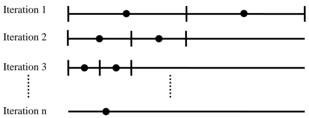
5.2 Binary Search Algorithm

The binary search algorithm is to find an optimum solution from a space. The space, denoted by { ∏ }, is the possible combinations of cutoff points for all products.

The algorithm is an iterative process. In an iteration, each product has two possible cutoff points to select. Taking a product route as a line, the two cutoff points are respectively on the first and the third quartiles (Fig 2). By evenly cutting the route into two sections, each cutoff point is in the middle of a particular section. Of the two evenly divided sections, the one where a cutoff point stays is called the housing

section of the point.

Iteration 1 Iteration 2 Iteration 3

Iteration n

In an iteration, the size of the space { ∏ } is if there are n products. By

solving the LP program times, we can obtain the best one--denoted by . For

each product, defines a particular cutoff point, whose housing section is called the

current

2n

2n Π*

*

Π

λ -section of the product. Theλ -sections obtained in an iteration is the input of the next iteration. The binary search algorithm is summarized below.

Algorithm Search _Cutoff_Points Initialization

z For each product, take the whole route as itsλ -section.

For iteration = 1 to N

z Create the two cutoff points on the λ -section of each product

z Solve LP programs to find Π *

z Compute theλ -section for each product based on Π *

End for

Chapter 6 Module 2—Queueing and GA

The problem to be solved in Module 2 can be stated as follows. Given a target

cycle time (CT₀) and a cutoff point decision (

1

* *

[π ,...,πn]

Π = ) obtained from Module

1, we attempt to find an optimal route ratio decision R=[ ,... ]r₁ rn in order to

maximize the total throughput of the two fabs subject that the corresponding cycle

time is less than CT₀.

This problem is essentially a space search problem, with a solution space

1

{ } {[ ,... ] |n _i ( , , ,_{i i i i})}

H= R = r r r = a b c d . A genetic algorithm is proposed to solve the

problem. In the algorithm, the fitness (performance) of a solution R is evaluated by a queueing network model. We first introduce the queueing network model and proceed to the genetic algorithm.

6.1 Queueing Network

The queueing network model is an extension of the model developed by Connors

et al. (1996). The I/O function of the model developed by Connor et al. (1996) can be

briefly formulated as follow: CT= f TH R( , ,Π . That is, given a total throughput )

(TH), a route ratio decision (R), and a cutoff point decision (Π ), the model can

compute the two fabs’ mean cycle time (CT). However, Connor et al. (1996) did not

consider the effect of transportation on CT.

We extended the application of their model based on two assumptions. First, we assume that the transportation path between any two stations is unique, where a station is either a workstation or a WIP storage buffer. Secondly, each transportation path between any two stations is modeled as a “conveyor machine” with only one unit of capacity. Such an extension makes the developed queueing model closer to the real

world. Likewise, the I/O function the extended queuing model can also be described as CT= f TH R( , ,Π).

The objective function in Module 2 is to maximize throughput (TH) subject to a

target cycle time (CT0). To evaluate the objective function, we used a bi-section

search technique to find the total throughput (TH) for a particular route ratio (R); that

is * where

0

( , , )

TH = f R Π CT Π denotes the cutoff point decision obtained in *

Module 1 and is the target cycle time. The bi-section search technique denotes

searching a value for TH, based on the function

0

CT

*

( , ,

CT= f TH R Π for a given R, in )

order to obtain ; and the search algorithm is just like that of the binary

search for a particular point on a line segment.

0

CT CT=

6.2 Genetic Algorithm

The genetic algorithm (GA) is to identify an optimal solution R* from the space

S = {R}. As stated, the performance of R is obtainable by the enhanced queueing model. A possible solution R (or called a chromosome) is represented by a vector

1

[ ,... ]n

R= r r where ri =( , , ,a b c di i i i). We call ri a gene-segment and each of its

element a gene, and the gene values are imposed by the following constraints:

and 0 .

1

i i i i

a + + + =b c d ≤a b c d_i, , ,_{i i i} ≤1

The GA is an iterative algorithm which can be briefly described as follows. Procedure GA

Step 1: Initialization

z t = 0, Status = ‘Not-terminate’

z Randomly generate N_pvalid chromosomes to form a population P0

Step 2: Genetic Search

z Use cross-over operator to create N_c new chromosomes

z Use mutation operator to create N_m new chromosomes

z Form a pool by the union of Ptand the newly created chromosomes

z t = t + 1, and select the best N_pchromosomes from the pool to form Pt

z Check if termination condition is met; if yes, set Status = “Terminate” Endwhile

Step 3: Output the best chromosome R* in Pt

The crossover operation is to create two new chromosomes (say, R3and R4) from

two existing ones (say, R1 and R2). Let each gene-segment i in R1 and R2 be

respectively represented by r_i1 and r_i2 . We proposed a one-point crossover

operation (Binh & Lan 2007) on gene-segments r_i1 and r_i2 to create two new ones

3

i

r and r_i4 , which in turn could yield two new chromosomes: R₃ =[ ]r_i3 ,

4 [i4], 1

R = r ≤i≤n.

The one-point crossover operation on a gene-segment is briefly introduced. For

two gene-segments (i.e., ri1 and ri2 ), randomly choose a gene, swap their gene

values, and modify another gene values in order to ensure a constraint satisfaction .

Consider an example where the second gene is chosen for r_i1=(a b c d_i1, _i1, _i1, _i1) and

2 ( 2, 2, 2, 2)

i i i i i

r = a b c d . By the swap and modification operations, we would obtain

3 ( 1, 2, 1,1 1 2 )

i i i i i i i

r = a b c −a −b −c₁ and r_i4 (a_i2,b_i1,c_i2,1-a_i2 -b_i1-c_i2).

In the mutation operation, a new chromosome (say, R2).is created by an existing

one (say, R1). The mutation algorithm creates R2 by modifying a particular

selected, two of its genes are randomly chosen and their gene values are swapped.

For example, if gene-segment i* is chosen for modification; and the 2nd and 4th

genes are chosen to swap for r_i*₁ =(a b c d_i1, _i1, _i1, _i1), then r_i*₂ =(a d c b_i1, _i1, _i1, _i1), which

in turn yield a new chromosome R₂ =[ ,..r₁₁ r_i*₂,...rn1] from R₁=[ ,..r₁₁ r_i*₁,...rn1].

Two termination conditions are defined for the GA. First, the best solution in Pt

has been no change for over a certain period (say, Tb iterations). Second, the

population Pt has evolved over a certain iterations; that is, t has reached its predefined

Chapter 7 Experiments

7.1. Benchmarks and Data

By numeric experiments, we attempt to evaluate the effectiveness of the proposed method. Two other methods are used as benchmarks for comparison. The proposed method is designed as LP-GA, where LP denotes the linear program, GA denotes the genetic algorithm. The two benchmark methods are special cases of

LP-GA. The first one is called M-GA, which denotes that the cutoff point of each route has been predetermined—just on the middle of the route. The second one is called

N-GA, where denotes that cross-fab production is not allowed. Such a comparison is

to tell how much benefit a dual-fab would obtain if the LP-GA method is used.

In the dual-fab experiments, the data for machines and product routes are adapted from an HP-fab in literature ( Wein 1988). Of the two fabs, one involves 93 machines and the other involves 72 machines. Being functionally identical, each fab involves 4 batch workstations and 21 series workstations. The MTBF (mean time between failure) and MTTR (mean time to repair) of each machine is available, exponentially distributed. Three types of products are produced. One product involves 150 operations; the other two both involve 172 operations but are different in

processing times. In implementing the GA, we set Tb = 1000, Tu = 30, P0 = 100, Pcr =

0.8, and Pm = 0.1.

7.2 Performance Comparison

The three methods are compared in two scenarios, with product mixes RA =

(3:2:5) and RB = (5:4:1) respectively. For each product mix, by the queueing model,

we obtain a throughput level that will keep the two fabs in high utilization: Q

B

A = 128

We compare the three methods from two perspectives. First, given a target throughput level, the mean cycle time of each method is compared. In the comparison,

QAand QB are used as the target throughput levels. Second, given a target cycle time,

we compare the throughput of each method. In the comparison, we set CT

B

0 =11081

min. for RA and CT0 =11445 for RBB.

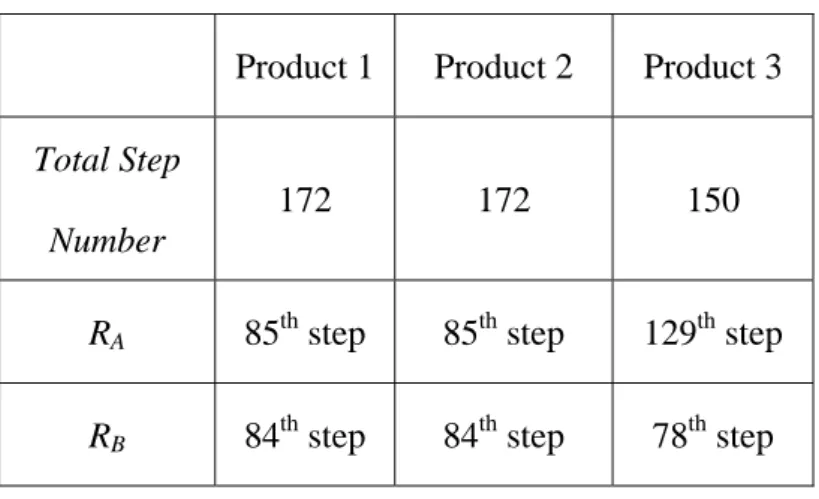
The cutoff points of each route obtained by the LP-GA method are shown in Table 1, which indicates that the cutoff points suggested by the LP-GA are different from that of M-GA.

Table 2 shows the comparison of mean cycle times, subject to a target throughput. The LP-GA outperforms the two benchmark methods. The cycle time of the LP-GA method is about 2-9% lower than that of M-GA, and 11-17% lower than that of N-GA. This implies that optimal planning of cross-fab production is positive in reducing cycle time.

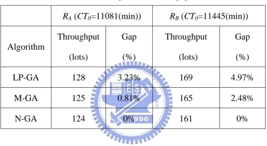
Table 3 shows the comparison of throughput, subject to a target cycle time. The

LP-GA method also outperforms the two benchmark methods. The throughput of the

LP-GA method is about 0.8-2.5% higher than that of M-GA, and about 3.2-5.0% higher than that of N-GA. This implies that optimal planning of cross-fab production is positive in increasing throughput.

Table 1: Cutoff points obtained by the LP program

Product 1 Product 2 Product 3

Total Step Number

172 172 150

RA 85th step 85th step 129th step

RBB 84

th

Table 2: Comparison of mean cycle time

RA(QA = 128 (lots)) RB (QB = 169 (lots)) B

Algorithm CT (min) Gaps (%) CT (min) Gaps (%)

LP-GA 11,080 11.10% 11,639 17.30%

M-GA 12,175 2.31% 12,811 8.98%

N-GA 12,463 0% 14,075 0%

Table 3: Comparison of throughput

RA (CT0=11081(min)) RB (CTB 0=11445(min)) Algorithm Throughput (lots) Gap (%) Throughput (lots) Gap (%) LP-GA 128 3.23% 169 4.97% M-GA 125 0.81% 165 2.48% N-GA 124 0% 161 0%

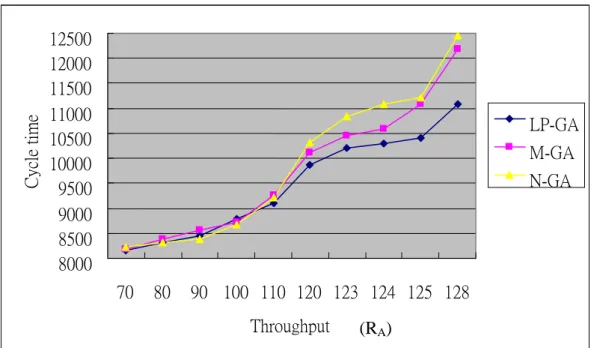
Figs. 3 and 4 reveal the relationship between cycle time and throughput for RA

and RB respectively. The higher the throughput, the longer is the cycle time. The two

figures also show that the higher the throughput, the larger is the performance gap. That is, the contribution of the LP-GA method becomes higher while it is applied in a high-demand scenario.

8000 8500 9000 9500 10000 10500 11000 11500 12000 12500 70 80 90 100 110 120 123 124 125 128 Throughput Cycle t ime LP-GA M-GA N-GA (RA)

Fig 3: Relationship between throughput and cycle time for product mix RA

7500 8500 9500 10500 11500 12500 13500 14500 80 _{100 120 140 160 162 166} Throughput Cycle time LP-GA M-GA N-GA (RB)

Chapter 8 Conclusion

This paper presents an approach to solve the route planning problem for a semiconductor dual-fab. In the problem, each product can be manufactured in either fab. And each product has four possible production routes, which are defined by a cutoff point. The route planning problem involves two decisions—determining the cutoff point and route ratio for each product—in order to maximize the throughput subject a cycle time constraint.

An LP-GA method is proposed to solve the route planning problem. We first use the LP module to make the cutoff point decisions, and proceed to use the GA module for making the decision of route ratio. The LP-GA method is compared with two benchmark methods by numerical experiments. Results show that the LP-GA method significantly outperforms the other methods.

Some extensions of this research are being considered. One is the extension of this approach to a multiple-fab production system—for example, three or more fabs shall share the capacity in production. The other is the extension to a scenario with higher flexibility in production routes—for example, each product could have two cutoff points and in turn have more than four routes.

Acknowledgements: This research is financially supported by National Science Council, Taiwan, under a contract NSC-90-2622-E009-001.

References

Binh. Q.D. and Lan P. N., “Application of a genetic algorithm to the fuel reload optimization for a research reactor,”Applied Mathematics and Computation, 187, pp. 977-988, 2007.

Connors D.P., Feigin G.E., Yao D.D., “A Queueing Network Model for Semiconductor Manufacturing,” IEEE Transactions on Semiconductor Manufacturing, 9, No. 3, pp. 412-427, 1996.

Defersha F.M. and Chen M., “A comprehensive mathematical model for the design of cellular manufacturing systems,” Int J. Production Economics, 103, pp. 767-783, 2006.

Frederix F., “An extended enterprise planning methodology for the discrete manufacturing industry,” European Journal of Operational Research, 129, pp. 317-325, 2001.

Karabuk S. and Wu S.D., “COORDINATING STRATEGIC CAPACITY PLANNING IN THE SEMICONDUCTOR INDUSTRY,” Operations Research, 51, pp. 839-849, 2003.

Kim C.O., Beak J.G., Jun J., “A machine cell formation algorithm for simultaneously minimising machine workload imbalances and inter-cell part movements,” Int J. Adv

Manufacture Technology, 26, pp. 268-275, 2005.

Lee M.K., Luong H.S., Abhary K., “A genetic algorithm based cell design considering alternative routing,” Computer Integrated Manufacturing Systems, 10, No. 2, pp. 93-107, 1997.

Lee Y.H., Chung S., Lee B., Kang K.H., “Supply chain model for the semiconductor

industry in consideration of manufacturing characteristics,” Production Planning ＆

Control, 17, No. 5, pp. 518-533, 2006.

ManMohan S.S., “Managing Demand Risk in Tactical Supply Chain Planning for a Global Consumer Electronics Company,”Production and Operations Management, 14, No. 1, pp. 69-79, 2005.

Nsakanda A.L., Diaby M., Price W.L., “Hybrid genetic approach for solving large-scale capacitated cell formation problems with multiple routings,” European

Journal of Operational Research, 171, pp. 1051-1070, 2006.

Rupp T.M. and Ristic M., “Fine planning for supply chains in semiconductor manufacture,” Journal of Materials Processing Technology, 107, pp. 390-397, 2000.

Toba H., Izumi H., Hatada H., Chikushima T., “Dynamic Load Balancing Among Multiple Fabrication Lines Through Estimation of Minimum Inter-Operation Time,”

IEEE Transactions on Semiconductor Manufacturing, 18, No. 1, pp. 202-213, 2005.

Vin E., Lit P.D., Delchambre A., “A multiple-objective grouping genetic algorithm for the cell formation problem with alternative routings,” Journal of Intelligent

Manufacturing, 16, pp. 189-209, 2005.

Wein L. M., “Scheduling Semiconductor Wafer Fabrication,” IEEE Transactions on

Semiconductor Manufacturing, 1, No. 3, pp. 115-130, 1988.

Wu M.C., and Chang, W.J., “A short-term capacity trading method for semiconductor fabs with partnership,”Expert systems with application, 33, No. 2, pp. 476-483, 2007.

Wu S.D., Erkoc M., Karabuk S., “MANAGING CAPACITY IN THE HIGH-TECH INDUSTRY: A REVIEW OF LITERATURE,”The Engineering Economist, 50, pp. 125-158, 2005.