Author(s): Weijing Wang and Martin T. Wells
Source: Journal of the American Statistical Association, Vol. 95, No. 449 (Mar., 2000), pp. 62-72
Published by: American Statistical Association Stable URL: http://www.jstor.org/stable/2669523 .
Accessed: 28/04/2014 04:17
Your use of the JSTOR archive indicates your acceptance of the Terms & Conditions of Use, available at .
http://www.jstor.org/page/info/about/policies/terms.jsp
.
JSTOR is a not-for-profit service that helps scholars, researchers, and students discover, use, and build upon a wide range of content in a trusted digital archive. We use information technology and tools to increase productivity and facilitate new forms of scholarship. For more information about JSTOR, please contact [email protected].
.
American Statistical Association is collaborating with JSTOR to digitize, preserve and extend access to Journal of the American Statistical Association.
Model Selection and Semiparametric Inference for
Bivariate Failure-Time Data
Weijing WANG and Martin T. WELLS
We propose model selection procedures for bivariate survival models for censored data generated by the Archimedean copula family. In route to constructing the selection methodology, we develop estimates of some time-dependent association measures, including estimates of the local and global Kendall's tau, local odds ratio, and other measures defined throughout the literature. We propose a goodness-of-fit-based model selection methodology as well as a graphical approach. We show that the proposed methods have desirable asymptotic properties and perform well in finite samples.
KEY WORDS: Archimedean copula; Bivariate survival function; Frailty distribution; Kendall's tau; Model selection; Odds ratio estimation; Time-dependent association.
1. INTRODUCTION
In recent years substantial research effort has been de- voted to developing methodology for multivariate failure- time data. Applications of multivariate survival analysis arise in various fields. Examples in biomedical applications include lifetime analysis in match-paired case control stud- ies, studies of time to occurrence of a disease to paired organs, and the examination of duration times of critical stages of a multistage disease process. Specifically, in Sec- tion 4 we consider an assessment of the effect of a medical intervention on angina pectoris. Danahy, Burwell, Aranow, and Prakash (1977) collected data on 21 cardiac disease pec- toris and recorded exercise time until angina pectoris and the exercise time until angina pectoris 3 hours after tak- ing oral isosorbide dinitrate. One needs to account for the censoring induced by patient fatigue. It is clearly important to assess the bivariate relationship between the control and treatment times while accounting for within-subject depen- dence, and a marginal analysis would not yield the impor- tant treatment effect information. As for other applications, in demographic studies of the dynamics of mortality, mul- tivariate models incorporate an exchangeable dependence structure by the inclusion of a cluster-specific random ef- fect (see Vaupel, Manton, and Stallard 1979). In engineer- ing applications, modeling the multivariate nature of me- chanical or electronic components in a parallel or a serial system has become increasingly important (see Marshall and Olkin 1988). The canonical problem of interest is to study the dependence relationship among several lifetime random variables. In many applications, it is often believed that the level of association varies across time, and it is of particular interest to investigate the time-dependent asso- ciation. In this article we focus on the bivariate case, al- though many of the ideas could be extended to multivariate problems.
Weijing Wang is Associate Professor, Institute of Statistics, National Chiao-Tung University, Hsin-chu, Taiwan (E-mail: [email protected]. edu.tw). Martin T. Wells is Associate Professor, Department of Social Statistics, Cornell University, Ithaca, NY 14851. The support of The Na- tional Science Council (grant 87-2118) and National Science Foundation (grants DMS 9625440 and 9971586) is gratefully acknowledged, as are the kind and helpful comments of the editor, associate editor, and refer- ees. The authors thank Phillip Hougaard for providing the references for the datasets.
Let (X, Y) be the lifetime variables of interest with joint survival function F(x, y) = Pr(X > x, Y > y)
and marginal survival functions Fi (.) (i = 1, 2). If the components of (X, Y) are locally independent at a point (x, y), then F(x, y) = Fi (x)F2(y). Hence the most simplis- tic method of assessing local dependence is by checking whether F(x, y)/{Fi (x)F2(y)} = 1. There exist many other time-dependent association measures constructed for differ- ent purposes of analysis; these include the local odds ratio function, the local Kendall's tau function (Oakes 1989), and the covariance function of the marginal martingale com- ponents (Prentice and Cai 1992). Anderson, Louis, Holm, and Harvald (1992) have given a nice general discussion on these measures.
A more modern approach to investigating local depen- dence is through model fitting. Although more assumptions may be required, modeling provides a systematic way to summarize joint relationships. The past decade has seen a substantial research effort toward deriving a unified ap- proach to studying models that are generated by a system of random effects. For example, Hougaard (1986) and Oakes (1989) discussed a family of correlated bivariate distribu- tions induced by a latent frailty variable. Lindeboom and Van Den Berg (1994) and Marshall and Olkin (1988) stud- ied a class of distributions generated by bivariate mixtures. Applications of frailty models were discussed by Bandeen- Roche and Liang (1996), Clayton and Cuzick (1985), Mur- phy (1994), Nielsen, Gill, Andersen, and Sorenson (1992), and Vaupel et al. (1979). Genest and MacKay (1986), Genest and Rivest (1993), and Joe (1993) studied the mathemati- cal properties of the copula and Archimedean copula (AC) classes. The copula class separates the dependence struc- ture from the marginal effects. Following development of the general modeling techniques, there has been growing research interest in developing methodology for selecting a particular model from a given class. For instance, Oakes (1989) used the local odds ratio function to identify the un- derlying frailty distribution. Genest and Rivest (1993) de- rived a measure based on a decomposition of Kendall's tau statistic to identify a particular AC model. However, in the
( 2000 American Statistical Association Journal of the American Statistical Association March 2000, Vol. 95, No. 449, Theory and Methods
important case where censoring is present, there have been no results to date.
Censoring is common in the analysis of lifetime data. In bivariate survival analysis (X, Y) may both be subject to censoring, this complicates the construction of statisti- cal inference procedures. Specifically, let (Cl, C2) be the nuisance censoring variables. With right-censored data, one observes (X,Y) = (X A C01,Y A C2) and a pair of in- dicators, (61,62) = {L(X < CI), II(Y < C2)}, where
a A b = min(a, b) and IL() is the indicator function. Re- cently, tremendous effort has been spent on the derivation of nonparametric estimators of F(x, y) for bivariate cen- sored data. Estimators of F(x, y) have been proposed by Campbell and Foldes (1982), Dabrowska (1988), Lin and Ying (1993), Prentice and Cai (1992), Tsai et al. (1986), van der Laan (1996), and Wang and Wells (1997), to name just a few. In this article we show how previous results can be used to derive inferential methods for parameter esti- mation and model selection. The proposed methods, which utilize the von Mises functional technique of Gill (1989), provide a unified inferential approach for estimating quan- tities that can be expressed as statistical functionals of F. Because the censoring issue is handled in the stage of es- timating F, the proposed approach is sufficiently flexible to deal with various censoring mechanisms. Extra informa- tion about the marginal distributions or covariates can eas- ily be incorporated into the analysis through the estimation of F.
In Section 2 we develop the theory for a new goodness- of-fit procedure and propose a graphical method to select a particular AC model for bivariate censored data. In Section 3 we derive an estimator of the local odds ratio function for models in the AC class. We present two real data analyses and simulation results on model selection in Section 4, and give some concluding remarks and point out some direction for further study in Section 5. We provide the proofs of the results in an Appendix.
2. MODEL SELECTION METHODS 2.1 Definitions
Many well-known bivariate lifetime distributions with continuous marginals, such as those proposed by Clayton (1978), Frank (1979), Gumbel (1960, 1961), and Hougaard (1986), are of the form
F (x, y) = Cc, {F, (x), F2 (y)}(1
where F(., ) denotes the joint survival function of (X,Y),Fi(.) (i = 1,2) are the marginal survival func- tions of X and Y, and Ol c Rk denotes an unknown asso-
ciation parameter. Note that the copula function, C(., ), is itself a survival function on [0, 112. A special fea-
ture of the copula class is that the dependence struc- ture is separated from the marginal effects, so the depen- dence relationship can be studied without specifying the marginal distributions. The parameter Ol can be viewed as
a global association parameter related to Kendall's tau,
specifically
T= 4J F(x, y)F(dx, dy)-1
4
j
C,(s, t)Cc,(ds, dt) - 1.Given the same level of overall association measured by Ol or T, C, (s, t) determines the degree of local dependence at (s, t) c [0, 112, where (s, t) indicates the joint survival status.
Note that all of the models reduce to the same form when the overall association approaches to the extreme levels, under independence (r = 0), C(s, t) = st and under positive maximal dependence (r = 1), C(s, t) = s A t, the upper Frechet bound (see Marshall and Olkin 1988).
Recent research has focused on a subclass of (1), the AC class, which indexes Cc,(., -) by a univariate function and thus has more tractable analytical properties. The survival functions in the AC class are of the form
F(x, y) F, (x) I + cF2(y) }], (2) where 0,(.) is a convex function defined on [0, 1] satisfy- ing 0a(1) = 0. This class also contains many useful mod- els, including the bivariate frailty family when f (.) is the Laplace transform of the underlying frailty distribution (Oakes 1989). Genest and Rivest (1993) showed that the function 0bc (.) in (2) can be recovered by the estimable uni-
variate function K(v) -- Pr{F(X, Y) < v}. Specifically, K(v) is related to 0b(.) through the differential equation
A(v) = v-K(v) Oa (v) (3)
where v$ (v)= t (v) /lv. The foregoing expression yields the inversion formula
q05(v) =exp I idt exp [o At t (4) [J 0 t - K(t) J i0 A (t)
where 0 < vo < 1 is an arbitrary constant. Thus K(v), or, equivalently A(v), plays a key role in the identification of qa(.), which in turn determines the underlying depen- dence structure for the AC class. The function K(v) has a general geometric interpretation related to contour analysis. Define the contour curve of F(., ) at level v for v c [0,1] by 4 (v) {(x, y): F(x, y) = v, (x, y) EE R2}. Because F(.,) is monotone, K(v) measures the mass between the contour curves Ob(0) and 0b(v). Equation (4) implies that members in the AC class are classified according to the distribution of the mass within the contour curves.
2.2 Estimation of K(v) Under Bivariate Censoring When the data are complete, Genest and Rivest (1993) proposed estimating K(v) by constructing "pseudo obser-
vations" of Vi = F(Xi,Yi) by VKi = E 1 I(xj > Xi,yj >
Yi)/(rn - 1) (i = 1,... n) and then estimating K(v) by
the empirical distribution function of the Vi (i n1,... n). Specifically, Genest and Rivest's estimate of K(v) is given by K(v) L>,= l(l7i ? v)/nt. This approach is not vi- able if some of {(Xi, Yi),i =1, ... .,rn} cannot be directly observed due to censoring. Here we propose an estimator
of K(v) for bivariate censored data, {(Xi, Yi, 61i, 62i), i 1,... n}. Consider the following expressions of K(v):
K(v) E[]L{F(X, Y) < v}]
j j
I 1[F(x,y) < v]F(dx,dy), (5) which can be estimated nonparametrically by plugging in an estimator of F in the foregoing integral form. Specifically, let <(l) ? < x(n) and <(1) ? < Y(n) be ordered observations of {(Xi, Yi), i = 1, ... . n}. The first proposed estimator of K(v) is given byK(v) J J1
[F(x,
y) < v]F(dx, dy)n n
-E
E
3
{F(x>,y) < v}F(A\(i),A\(j)), (6)i=1 j=1
where F is a nonparametric estimator of F and F(\Ax(i), Ay(j)) =F(x(), Y(j)) - F((-) i) Y(j)) - , +(x(i) Y(j_i)) ?
is the estimated mass at (x(i), (j)). When there is no censoring, F(xi,yi) =
Ln
1(xj > xi, yj > yi)/n, (i - l,... n), is the empirical survivalestimate at (xi,Yi),F(Axi,Ayi) = 1/n (i = 1,.. , n) and F(A\xi,Ayj) = 0 if i =8 j. It is easy to see that K(v) - K(v) = 1/n En IL [v < Vi < (n/n - I)v] -?P
Pr(F(X, Y) = v), which equals 0 under (2) and the assumed continuity (Genest and MacKay 1986). Hence K and K are asymptotically equivalent in the case of no censoring.
The nonparametric estimators of F mentioned previously were all derived under the assumption that (X, Y) are in- dependent of (Cl, C2). Sometimes the independent censor- ing assumption is not plausible. Lin, Sun, and Ying (1999), Visser (1996), and Wang and Wells (1998) discussed a de- pendent censoring situation when (X, Y) are the duration times for successive events and proposed nonparametric es- timators to adjust for dependent censoring. Note that be- cause the issue of censoring is handled in the stage of esti- mating F, the proposed idea for estimating K(.) is flexible under various censoring structures as long as an appropriate estimator of F is used.
Properties of K(v) depend on properties of the under- lying estimator F. Denote the support of (X, Y) by f = {(x,y): Pr(X > x,Y > y) > 0}, and let V be the im- age of f under F. Under right censoring, f is contained in the support of (X, Y). Asymptotic results for most non- parametric estimators of F are valid only for points in f, the restricted support. Because F(x, y) cannot capture the mass outside f, K(v) must be modified. The modified estimator of K(v) is based on the equivalent expression, K(v) = - Pr(F(X, Y) > v), and is given by
n n
K (v) = I1-
E
L [FP(x~(i), ) w) > vIi=1 j=l
The following theorem shows that if the underlying esti- mator of F is consistent and converges weakly to a Gauss-
ian process on D[T], then K(v) will inherit some nice properties on D[V]. The weak convergence (X~) result for xf/;i{K(v) - K(v)} has been established by Barbe, Genest, Choudi, and Remillard (1996) for complete data. To deduce the weak convergence result for vf/i {K(v) - K(v) } we need
the following hypotheses:
H1. The distribution function K(v) of V = F(X, Y) admits a continuous density k(v).
H2. Given F(x, y) = v, there exists a version of the con- ditional distribution of (X, Y) and a countable family P of partition C on f into a finite number of Borel sets satisfying infcEP maxCEC diam(C) = 0, such that for all C
c
C, the mapping v -? ,i (C) = k(v) Pr{(X, Y) E CIF(X, Y) = v},is continuous.
Theorem 1. If F(x, y) is a uniformly and strongly con- sistent estimator of F(x, y) for (x, y) c T, then for 0 <
F(71,72) < v < 1 with (T1,72) E T,K(v) 4 K(v) on
[(,1] . Furthermore, if nl /2 {F(x, y) - F(x, y)} => W(x, y),
where W(x, y) is a continuous mean-zero Gaussian process on D[7], then under Hi and H2, it follows that on D[(, 11, n 1/2{k(v) - K(v)} :# X(v) - l
(F
(x, y) > v)x W(dx, dy) -
JJ
W(x,
y)1 u(dx, dy).The weak convergence of various estimators of F was demonstrated by Gill, van der Laan, and Wellner (1993) using functional delta-method theorems to establish func- tional central limit theorems. (For an extensive weak con- vergence theory, see Gill 1989 and van der Vaart and Well- ner 1993.)
The asymptotic variance of k(v) depends on the asymp- totic variance of F. However, in general it is too com- plex to give a closed-form expression of the asymptotic variance for most estimators of F. Therefore, the boot- strap method becomes a practical alternative for obtaining the variance estimate (Dabrowska 1989). Specifically, let
{ (X*j,Yj** v lv R jj = 1 ... m} be a random sample with
replacement from the original data {(Xi, Yi, 31i, 32i), i
l,...,rn} and let F*(x, y) and K* (v) be the bootstrapped counterparts of F(x, y) and K(v). Using a functional delta- method theorem of Gill (1989), it can be shown that as mAn -X o0, the bootstrap process ml/2{F*(x,y)-F(x,y)}
converges to the same limiting process as nr/2{F(x, y) -
F(x, y) }. A similar argument may be applied to show that the bootstrap version, ml/2 {k* (v) - k(v)}, also converges
to the same limit of nr/2{K(v) - K(v)}.
Once an estimator of K(v) is obtained, fb(.) can be esti- mated nonparametrically by using the inversion formula in (4); that is,
0(v) = exp
[]
K( cdt1 . (8)Because K(v) is a step function, to evaluate (8), one must smooth K(v) and then perform numerical integration. How- ever, in general eb(v) does not have a tractable form. For
inferential purposes, it is more appealing to select a para- metric family of 0bc(.) that best describes the data. The following section introduces a goodness-of-fit statistic for testing whether the data are drawn from a hypothesized model.
2.3 Goodness-of-Fit Statistics
A number of metrics could be used as goodness-of-fit statistics to measure the discrepancy between a hypothe- sized model and the empirical model. A natural choice is the L2-norm distance,
S((a) K{K(v) - K,(v)}2 dv. (9)
Note that to evaluate Kc (.) for the hypothesized model, one usually needs to estimate ae. A preliminary estimator of ae may be obtained via an estimator of Kendall's tau based on the relationship
T 4E[F(X, Y)] -1 =
4j
a(v)
dv + 1_ A((a).(10)
If A(c) = r is a one-to-one function, then ae can be esti- mated by &z = A-l(r), where -r is an estimate of r. If ris not a one-to-one function of ae, then some artificial con- straints may be imposed. For example, the log-copula model is indexed by two parameters, ae and ay (see Table 1), and for
convenience, one may assume that ay = 1. Nonparametric estimation of Kendall's tau under censoring is a complex problem. It turns out the estimators proposed by Brown, Hollander, and Korwar (1974) and Oakes (1982) are not consistent if T =6 0. Wang and Wells (1999) showed that if the largest observations, x(n) and Y are both uncensored, then
n n
to= 4 , (j() I Y()F/z()\(j) )1 ()
i=1 j=1
is a consistent estimate of T. However, in general io -
4 fT F(x, y)F(dx, dy) - 1 < T. Alternatively, ae can be estimated by using a minimum distance-type estimate & = argminc. f {K(v) - K&(v)}2 dv. Similar types of minimum Cramer-von Mises estimates were discussed by Shorack and Wellner (1984, p. 254). The following theorem sum- marizes the asymptotic properties of oe.
Theorem 2. If K (v) is twice differentiable with re- spect to ae with bounded derivatives and rn{K(v) - K&(v)} => X(v), where X(v) is defined in Theorem 1, then nl /2 (&a-o) converges in distribution to [f{ [aKc, (v)] /&aa2 dv] - 1 f(Ka (v)/&cl)X(v) dv.
The proof of Theorem 2 is given in the Appendix. Note that due to the complexity of X(v), it is also difficult to derive a closed-form expression of the asymptotic variance of oe. The bootstrap method discussed earlier can be used to obtain the variance estimate. Other semiparametric estima- tors of ce for copula models have been proposed by Genest, Ghoudi, and Rivest (1995), Hsu and Prentice (1996) and
Shih and Louis (1995). These estimators have the desirable properties, and the variance of their estimators can be esti- mated analytically.
The following two results supply the needed asymptotic theory for construction of the formal test procedure. The first is a simple consequence of the continuous mapping theorem (Shorack and Wellner 1986, chap. 5) for integrals of squared Gaussian processes.
Proposition 1. If rt{K(v) - K (v)} > X(v) on
D[,1], then n S(a) => f1 X2(v) dv.
With ae estimated by &, the ideas from the area of goodness-of-fit testing for a composite hypothesis may be applied (see Shorack and Wellner 1996, chap. 5).
Theorem 3. If Kc.(.) is twice differentiable with re- spect to ae with bounded derivatives and rt(& - ae) > Q,
where &z is an estimate of ae, then rti{K(v) - K&(v)} => X(v)- X(v) - [aKc,(v)]j/&aQ. Furthermore, nS(a) =>
fSX2(v) dv.
The asymptotic variance of S(&), denoted by s2, is also
difficult to estimate analytically. However, the naive boot- strap approach discussed earlier by resampling bootstrap replicates from the original sample, {(Xi, Yi, 6ii, 62i), i =
1, .. ., n}, is not valid for obtaining a reasonable estimate of jS. We give a heuristic explanation in the next section. Romano (1988) discussed the validity of using the boot- strap to approximate the asymptotic distribution of some general distance statistics. According to the general theory, in our case one generates a bootstrap sample, VI.*.., Vn
},
from the distribution V - K&(v). Using the fact that T = 4E(V) - 1, where V = F(X,Y), with the boot-strap sample one can compute K* (v)
L=~
,1 (Vi* ? v =4 U1 Vi*/r- * A-1(f *), Ko* (v)n and then S* (&z*) {K* (v) - K*(v)}2 . By repeating thebootstrap procedure many times, one can estimate a by the sample variance of bootstrap estimates of S* (&*). Note that it does not matter whether originally &z is obtained by inverting an estimate r or not, because the difference of nS(&) by using different consistent estimates of ae is of smaller order and hence negligible.
2.4 A Graphical Model Selection Method
Practitioners often need to select the best-fitting model among some competing model alternatives for the data at hand. Genest and Rivest (1993) proposed a graphical model selection procedure by plotting empirical estimates of A(v) = v - K(v) with theoretical curves of A,(v) for models under consideration. The best-fitting model is the one whose theoretical curve is closest to the empirical es- timates. The function A(v) can be estimated by A(v) = v - k(v). Plotting A(v) instead of k(v) gives a better
visual comparison between A(v) and A(v) than the differ- ence between K(v) and K(v). Note that because lk(v) -
K () = A(v) - A&,(v) l,K(v) and A(v) yield the same in-
formation measures.
The relative magnitude of the test statistic, S(o&), under different model assumptions can be used to rank the model
proposals. We need not include a model complexity penalty if the models under consideration all have roughly the same number of parameters. Note that because ae is estimated, c' depends on the form of Ka (v) and thus is different for different model hypotheses. It is not clear whether the stan- dardized statistic T(&) _ S(&)/us, which accounts for the variation of S(&), is a better measure for model selection than S (&). We find that the value of as is much smaller under the true model. To simplify the discussion, suppose that parameters of the model alternatives all have one-to- one correspondence with Kendall's tau. Denote KT (.) as the distribution function of F(X, Y) under the true model with the true T and K,-(.) as the function for any hypothesized model with the true level of r. It follows that
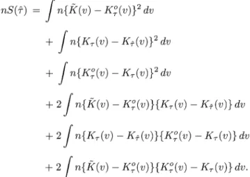
nSQ() J n{K(v)-K (v)}2 dv
+
J {Kr (v) -K_ (v)}2 dv+
J r{KT (v) -K (v)}2 dv + 2J nr{k(v) - K (v)}{K. (v) - K (v)} dv + 2J nm{K.(v) -K_(v)}{K,(v) -KT(v)}dv F 2J nr{k(v) - K (v)}{K, (v) - K (v)} dv.When the hypothesized model is the true one, Ko(.) Ko(.) and nrS(&) z> fk2(v) dv, as stated in Theorem 3.
However, if the hypothesized model is misspecified (i.e., K0(v) - Ko(v) = c(v) * 0, where c(v) is a constant vary- ing with v), then nS(Q) will diverge as n -X oc and pro-
duce large variation in finite samples. Because T(&) would impose an unnecessary penalty on the correct model, we suggest ranking the models based on S(&) and not on its standardized version.
The foregoing decomposition of nS(Q) can also be used to illustrate why the naive bootstrap procedure is not valid for estimating the asymptotic variance of nS(&). Although the naive bootstrap procedure provides a good approxima- tion of nr/2{k(v) - K-(v)} and n 1/2{K,(v) - K-(v)}, it
cannot mimic the behavior of nri/2{K (v) -K,(v)}. In sim- ulations, not presented here, we found that the variance estimate using the naive bootstrap method is much larger than its theoretical value, especially when the hypothesized model is the true model.
Table 1. Examples of 0 (v) Range of
Family qc(v) ae and ey O (v) Clayton (v-- 1)/cr (0, oo) ca+ 1 Frank log (, -exP(-ce) (- ?) 1 vc)
Gumbel {-log(v)} [o, oo) 1- a
Log-copula {1 - log (v)/coy}'a1- 1 (0, oc) 1 + alg I -Gaussian {log v} {log v- 2cE}/(2cE2 ) (0 , oo) 1 + 1
To simplify numerical analysis, S(ae) can be replaced by its Riemann sum approximate; that is, S(ae) -
Zi=i{K(v(i))- Ko(v(i))}2(v(i) - v(i_1)), where v0 = 0
and v(i) < n< v() are the ordered values of {Vj -
F G jj), j = 1, ... , n}. The proposed graphical model se- lection procedure that can handle bivariate censored data is described by the following steps: Select an appropri- ate plug-in estimator of F; compute k(v) and then A(v); plot A(v) = v - K(v) for v = F( (,p) (i = 1, .. ., n); esti-
mate ay, the parameter for the jth model, by &j; compare the empirical plot of A(v) with theoretical plots of A63 (v) for models under consideration; and choose a model that provides the closest fit to the estimated curve-that is, se- lect the model with smallest S(&j). Note that iterating the last two steps provides a visual way to obtain &, the es- timator that minimizes the L2 distance between K(v) and Ko(v).
3. ESTIMATING THE ODDS RATIO FUNCTION FOR THE ARCHIMEDEAN COPULA CLASS
The local odds ratio function first proposed by Oakes (1989) provides an intuitive way to describe local associa- tion, which is defined as
0* (X y) = F(x, y)DlD2F (x, y) (12) {DIF(x, y)}{D2F(x, y)}'
where Di (i = 1,2) denote -0/x and -O/Oy. In gen- eral, 0* (x, y) is a bivariate function measuring local de- pendence and equals 1 if (X, Y) are independent at (x, y). For (X, Y) in the AC class, Oakes showed that Q* (x, y) de- pends on (x, y) through some univariate function 0{F(x, y)} such that 0O(v) = -v{[0"q(v)]/[[' (v)]}, where (v)
fV
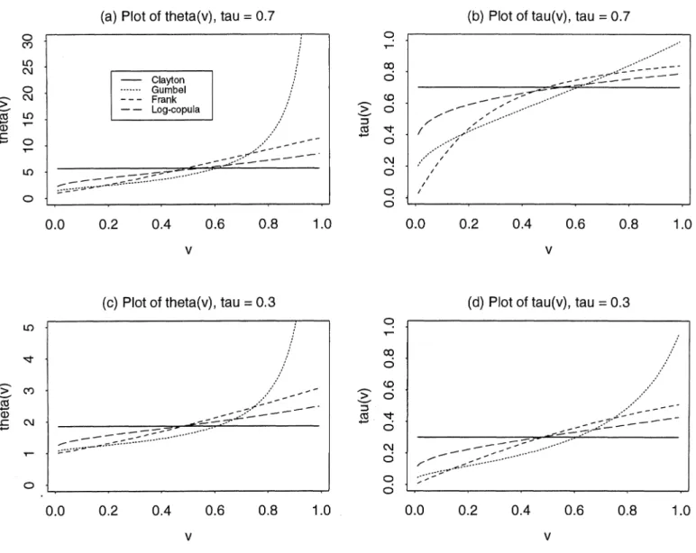
exp{f fC[0(u)/u] du} dz, where c > 0 is a constant. The form of 0a, (v) for several models in the AC class are listed in Table 1. (For more detailed properties of the odds ratio function, see Anderson et al. 1991 and Oakes 1989.) Oakes also derived another local dependence mea- sure, called local Kendall's tau and denoted by r(v), which is given by T, (v) = E[sign{(Xi -X2) (Y1 -Y2)} |X1 A X2 = x, Y1 A Y2 = y] = {[0 (v) - 1]/[0 (v) + 1]}, where v =F(x,y). Note that -1 < T(v) < 1. Figure 1 plots 0a(v) and m, (v) for several AC models. The patterns of 0, (v) and
,(v) are the same at two levels of r: r = .3 and r = .7. Larger values of 0(v) and r(v) indicate higher dependence. Because v represents the joint survival probability, as time passes, v changes from 1 to 0. It can be seen that for Gum- bel's type II model of extreme values (which has a positive stable frailty), 0(v) decreases exponentially as v decreases from 1 to 0, whereas for Frank's model and the log-copula model, 0(v) decreases fairly linearly. For Clayton's model, 0(v) and r(v) both stay at the same level. In fact, 0*(x,y) is a constant for all (x, y) for the Clayton model. When ,r = .3, the inverse Gaussian frailty model behaves like Frank's model, whereas it will approach Gumbel's model as 7 X~ .5 (not shown in Fig. 1).
Oakes (1989) proposed a nonparametric estimator of 0* (x, y) that applies only to discrete or grouped data. Based on (12), estimating 0* (x, y) for continuous distributions in-
(a) Plot of theta(v), tau = 0.7 (b) Plot of tau(v), tau = 0.7 o 0 C\J ~~~~~~Clayton - -- o Gumbel - ,: - \I - - Frank ( 1- 0 -- Log-copula > C _ - - 0. 0.-. . . . 0. 02 04 06 08 10 d0 _ -. 0 0 0 _________ 0.0 0.2 0.4 0.6 0.8 1.0 0.0 0.2 0.4 0.6 0.8 1.0 V V
(c) Plot of theta(v), tau .33 = 0.3 (d) Plot of tau(v), tau 0
10 ~~~~~~~0 co CZ C 0 0 0.0 02 0.4 0.6 0.8 1.0 0.0 0.2 0.4 0.6 0.8 1.0 V V
Figure 1.- Plots of Oc, (v) and i-r, (v). - Clayton, . Gumbel, - -- Frank, ---Log-copula. (a) theta(v), tau = .7; (b) tau(v), tau .7 (c) theta(v),
tau = .3; (d) tau(v), tau = .3.
volves estimating the derivatives of F(x, y). Let f(x, y) = DlD2F(x, y) be the joint density function of (X, Y). A simple kernel density estimator of f (x, y) for bivariate cen- sored data is given by fb(x, y) = 1/b2 En 1 En1 -({[x X(i)]/b}) {[y - y(j)]/b})F(zXx(i), \yj)' where 1(., ) is a
bivariate kernel function and b is a bandwidth parameter. Wells and Yeo (1996) discussed kernel density estimation for bivariate censored data. Estimates of DiF(x, y) and D2F(x, y) can be obtained by integrating f(x, y). There- fore, a nonparametric estimator of O* (x, y) for continuous (X, Y) is given by
O*(xy)
{f
f, fb3 (s, t) ds d!d
,b (X ({fxfbi (s Y) ds} {fy!2(t) dt}
where b, bl, b2, and b3 denote the bandwidth parameters for each component. Different bandwidths are used, because it is known that the optimal rate of convergence for the band- width of a kernel density estimator and a kernel estimator of an integral of a density are different. Thus 0*(x,y) re-
quires choosing different bandwidths for b, b1, b2, and b3. In a simulation study not shown here, we found that 0* (x, y) is very sensitive to the choice of bandwidths and the nor- malizing constants.
For models in the AC class, a simpler estimator of the odds ratio function can be derived. Let k(v) be the density of V = F(X, Y). It follows that k(v) =
{[q5(v)]/[q'(v)]}{[q"(v)]/[q'(v)]} = (K(v) - v)[0(v)/v] and hence 0(v) = {[vk(v)]/[K(v) - v]}. Note that the univariate density function k(v) can be estimated by
the kernel estimator, k(v) 1l/h
EnL1
E
1
4([v -F y(j))]/h)F( x(i), Mu)), where T(.) is a univariate kernel function satisfying the usual regularity conditions and h is a positive bandwidth parameter sequence. Hence 0 (v) can be estimated by 0 (v) = {[vk(v)] / [K(v) - v] }. Note that when v is close to 0 or 1, the performance of 0(v) will be less stable, because its denominator is close to 0. Un- der fairly weak conditions, k(v) is a pointwise consistent estimator of k(v), and hence 0(v) is a pointwise consistent estimator of 0(v). The proof of the next result is given in the Appendix. Theorem 4 can easily be shown by applying Theorem 1 and Proposition 2.
(a) Clayton(tau=0.7) (b) Clayton(tau=0.7),h = 0.25 o> -- "' -f - .l-i- - - 1. s < *ds B;,=~~~~~~~~~~~~~~~~~-.,_e---= # wA 4f? ij 'V">!s ,,... Gumb l 6
~ ~ ~ ~
. 0. 0. 0._. . . . o~~~~~~~~ 0 (eFFan(ank.)()Fakta=.)h=02 0 .2 0.4 0.6 0.8 1.0 0.2 0.4 0.6 0.8 1.0 V V (c) Clayton(tau=0.3) (d) Clayton(tau=0.3),h = 0.25 0 E -~7 0.2 04 06 08 0.2 0.4 0.6 0.8 v v(e) Frank(tau=0 7) (f) Frank(tau=0.7),h 0.25
N N
0008 1 000200601.
Fiue2C lt fEprcladHpteie A v.-Catn . ubl - rn, Lg-oua a lyo tu=.) b lyo
(tu .),h= 25 ()Clytn tu .);(d lato (a =.3, .5;(e rak ta =.);(f Fak ta =.),h .5
Proposition 2. Suppose that the kernel function '(.) is bounded and satisfies
f
I I(t) I dt < oo, f f (t) dt = 1, and ItQ(t)l - 0 as Itl - oo. Suppose that the bandwidthsequence satisfies h X 0 and nh -X oo as n -X oo. If
K(v) - K(v) on v E [(,1], then for v E ((, 1], k(v) 4 k(v).
Theorem 4. Suppose that K(v) - K(v) and k(v) -
k(v) for v E ((, 1], then 0(v) = {[vk(v)J/[K(v)-vJ} 4 0(v), for each v C(, 1].
4. NUMERICAL STUDIES 4.1 Real Data Examples
Two datasets were analyzed for illustrative purposes. Dabrowska's estimator was used as the plug-in estimator of F in computing k(v) and 0(v). The first dataset (Danahy et al. 1977), introduced in Section 1, was from a study on the length of exercise time required to induce angina pectoris for 21 heart disease patients. Here T1 is the exercise time to angina pectoris at time 0 and T2 is the exercise time to angina pectoris 3 hours after taking oral isosorbide dini-
trate. Only four observations of T2 were censored due to patient fatigue. The estimated value of r is .39 from Wang and Wells (1999) and .48 from Brown et al. (1974). It turns out that theoretical curves of A&(v) using & inverted from
r = .48 are farther away from the nonparametric estimates
of A(v) than those from using r = .39, which, however,
still may not be the best choice. After trying several values of , we found that the theoretical curves of A) (v) with o
inverted based on r .37 are closest to the empirical A(v).
By inverting from , .37, we obtained estimates of ae for
the models under comparison; the values (x O-4) of S(&) for the Clayton, Gumbel, Frank, and log-copula models are
12.47, 23.56, 17.29, and 13.27. This implies that the data more likely come from the Clayton model or the log-copula model than from the other two models.
The second dataset (McGilchrist and Aisbett 1991) was from a study of the recurrence time of infection in kidney patients using a portable dialysis machine. Two successive recurrence times, measured from insertion until the next in- fection, were recorded. The catheter must be removed if an infection occurs. After the infection clears up, the catheter
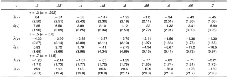
Table 2. Large-Sample Simulation Results for Frank's Model (Based on 1,000 Replications) v .3 .35 .4 .45 .5 .55 .6 .65 .7 r= .3 (a = .292) A(v) .04 -.61 -.83 -1.47 -1.22 -1.0 -.34 -.43 -.45 (2.50) (2.51) (2.43) (2.30) (2.19) (2.11) (2.01) (1.86) (1.66) a(v) 7.85 5.50 3.89 2.10 1.12 -.22 -1.32 -3.41 -5.90 (1.90) (2.09) (2.25) (2.34) (2.53) (2.72) (2.91) (3.09) (3.26) r= .5 (a = 5.8) A(v) -4.22 -2.99 -2.55 -2.57 -2.79 -2.11 -1.56 -1.36 -1.30 (2.27) (2.14) (2.09) (2.11) (2.13) (1.97) (1.86) (1.78) (1.68) a(v) 5.83 3.72 1.79 -.41 -2.73 -4.34 -6.67 -11.2 -18.5 (3.69) (3.69) (3.96) (4.34) (4.89) (5.15) (5.41) (5.72) (5.97) r = .7 (a = 1 1.5) A(v) -1.20 -2.14 -1.07 -.85 -1.29 -.77 -.69 -.71 -2.21 (1.71) (1.73) (1.77) (1.72) (1.78) (1.85) (1.74) (1.81) (1.75) 0(v) 258 189 143 85.6 29.6 -19.9 -76.3 -128 -189 (20.1) (19.4) (19.8) (20.0) (21.1) (20.8) (21.8) (21.7) (20.8)
NOTE: In each cell, the first row (X 103) is the average bias of A(v) and the second row (X 102) is the standard deviation of A(v). The third row (X 102) is the average bias of 0(v) and the fourth row (X 10) is the standard deviation of 0(v).
is then reinserted. Censoring may be due to removal for other reasons or the end-of-study effect (for the second in- fection). Let T1 be the time to the first infection, and let
T2 be the time to the second infection. There were 38 ob-
servations. Here 6 observations of T1 were censored, 12 observations of T2 were censored, and 3 observations were doubly censored. The estimate of r by Wang and Wells (1999) and by Brown et al. (1974) are both close to .21. Us-
ing & = A-1(r) with r = .21, the value (xlO-4) of Sn(&)
for the Clayton, Gumbel, Frank and log-copula models are 21.72, 11.23, 12.44, and 16.14. The result implies that the Gumbel model provides the best fit to the data.
4.2 Simulation Results
A series of simulation studies were carried out to investi- gate the performance of the proposed methods. In all of the simulations, we used an algorithm of Genest (1987) to sim- ulate the Frank model and an algorithm of Prentice and Cai (1992) to generate data from the Clayton model. In all of
Table 3. Large-Sample Simulation Results on S (Based on 200 Replications)
Frank Clayton Gumbel Log-copula Frank a 68.5% 1% 11.5% 19% T .3 b 2.6 9.6 5.0 4.5 c (1.5) (5.3) (2.7) (3.0) Frank a 84.0% 0% 7.5% 8.5% T .5 b 2.5 14.1 6.0 6.1 c (1.3) (5.4) (2.6) (3.0) Frank a 87.5% 0.5% 5.5% 6.5% -=.7 b 2.6 11.5 5.6 5.5 c (1.5) (4.5) (2.4) (2.6) Clayton a 1% 74% 0.5% 24.5% T .3 b 9.7 3.4 15.5 4.7 .c (5.7) (1.8) (7.0) (3.4) Clayton a 0.5% 84% 0% 15.5% T .5 b 14.7 3.2 23.5 5.8 c (6.42) (1.6) (7.6) (3.5) Clayton a 0% 80.5% 0% 19.5% T .7 b 11.2 3.3 18.3 4.2 c (4.8) (1.8) (5.6) (2.8)
NOTE: In each cell, the first row is the percentage of the column model being selected. The second row (X 104) is the mean of S, and the third row (X 104) is the standard deviation of S.
the cases, (Ci, C2) were generated from Clayton's model with T = .3, and the censoring rates in both components
were controlled to be between 10 and 20%. The sample size was n = 250. The Dabrowska estimator of F(x, y)was used as the plug-in estimator to compute K(v), k(v), A(v), and 0(v), and r and ae were estimated by & = A-1(r).
In computing k(v), we used the Epanechnikov kernel (i.e.,
(V) = 34[I - v2]L[Ivl < 1]), and set the bandwidth as h = .25.
Figure 2 shows the diagnostic plots of A(v) and 0(v) based on one sample replication when the true model is gen- erated from the Clayton and Frank models. The estimated curves in general can capture the shape of the true theoreti- cal curves. It should be noted that for Clayton's model, 0(v) is very unstable for v < .2. Table 2 presents summary statis- tics (based on 1,000 replications) of A(v) and 0(v) for the. Frank model. In general, A(v) has smaller bias and smaller variation than 0(v), which is reasonable because 0(v) in- volves estimating a density term that has a slower conver- gence rate. Note that as T increases, the standard deviation of 0(v) also increases. The bias of 0(v) for Frank's model also increases drastically when r .7.
The proposed model selection approach has been evalu- ated; Table 3 presents the results. The "best" fitted model that gives the smallest value of S(&) is selected, where ae for the jth model is estimated by &Oj = A- (l). It can be seen that when the fitted model is the true one, S(&) has the smallest mean and standard deviation. Table 3 shows that when r > .5, the probability of selecting the true model exceeds 80%. In the case when r = .3, the probability of
selecting the true model decreases to 70%. The log-copula model has the second-highest probability of being chosen when the true model is Frank's or Clayton's model. When the data are drawn from Clayton's model, it seems very un- likely to choose a Gumbel model. As we have seen from the univariate descriptive plots in Figure 1, when r is small, the
log-copula model is between Frank's model and Clayton's model, and the Gumbel model is very different from Clay- ton's but more similar to Frank's model. The results imply that the proposed model selection method can protect from
fitting a bad model. When T is small, the models become
more alike, so that the mistake of selecting a wrong model becomes less serious.
The bootstrap method discussed in Section 2.3 for esti-
mating o- was also evaluated. For a sample {(Xi, Yi,
a1i,
62i)1= ,... , n}, we estimated ae by & and then simulated
(V7*,...,Vn) from V - K&(v), which we then used to compute S* (&*). The bootstrap process was repeated 100 times. The sample standard deviation of S* (&*), denoted by &,, became an estimate of u?. When the true model was generated from the Clayton model, the sample means of &, (x104) based on 200 simulation replications were 1.99, 1.69, and 1.92 under r = .3,.5, and .7. When the true model was from Frank's model, the sample means of &, (x104) were 1.7, 1.56, and 1.66 under T = .3,.5, and .7. Compared with the true value of u? listed in the third row of each entry in Table 3, we find that &, tends to slightly overestimate o-v, but the bias is small.
5. CONCLUSIONS
In this article we have studied several model selection strategies for the class of Archimedean copula models with bivariate censored data. We expressed the important function K(v) as a statistical functional of the joint sur- vival function so that it can be estimated using the von Mises functional techniques discussed by Gill (1989). The proposed approach is quite flexible for adjusting various data-generating mechanisms. As mentioned previously, the plugged-in estimator F should account for the underlying censoring structure. Auxiliary information can also be in- corporated in the stage of estimating F. For example, if the marginal distributions are specified and can be estimated by Fi* (.) (i 1, 2), the plug-in estimator may be estimated by F(x, y) F, (x)F2 (y)f (x,y), where b(x, y) can be ob- tained nonparametrically based on a bivariate product limit expression of Dabrowska (1988) or an integral equation re- lated to the martingale covariance function of Prentice and Cai (1992). When covariate information is available, F may be estimated using the idea described by Prentice and Cai (1992).
APPENDIX: PROOFS
A.1 Proof of Theorem 1: Weak Convergence of ?n{K(v) - K(v)}
Assume that W(x, y) = {F(x, y) - F(x, y)} W(x, y),
where W(x, y) is a continuous Gaussian process on the space D[0, Ti] x [0, T2] with the Skorohod topology and F(Ti, T2)- >
0. One can write -y?{k(v) - K(v)} - &(v) + /3(v) + 7 (v),
where
&(v)
J
J
It(F(x, y) > v) VnZ{F(dx, dy) - F(dx, dy)},NO(v) Jv {I (F(x, y) > v) - IL(F(x, y) > v)}F(dx, dy), and
7(v)- J{IXt(F(x,y) > v)-X I(F(x, y) > v) }
x \iY{lt(F(dx, dy) > V)-l I(F(dx, dy) > v)}.
The proof contains three steps. Specifically, we show that a(v) =, f L(F(x,y) > v)W(dx,dy) =_ a(v),~(v) =>, f f W(x,y)wv(dx,dy) /3(v), and ry(v) o,(1). Let U1j_1Cj be a partition of [O, Ti] x [O,T2]. Define w(f, r) SUPd((x1,Y1),(X2,Y2))<r If (xi, yi)-f (X2, Y2) I to be the modulus of
continuity of f.
A.].] Part I: Proof of Weak Convergence of &(v). First, we show that &(v) converges in distribution to ae(v). The set {(x, y): F(x, y) > v} can be approximated by a union of disjoint rectangles. For any rectangular set, B -{(x, y): a < x < b, c < y < d}, the weak convergence of W(x, y) to W(x, y) implies that
fA fA W(dx, dy) = W(b, d) - W(b, c) - W(a, d) + W(a, c) >
ba fc W(dx, dy). Letting the mesh of rectangular grids become
finer, one can show that for each v E [(, 1], &(v) X oa(v). Fur- thermore, one can show that for any finite sequence (Vl,. . . , vI)
in [(, 1], the distribution of {(Vl),... ., &I(v ) } converges to that
o f{a(Vl), .. ., oc(viV)}. It remains to show that the process &(v) is tight, which can be proved by showing that for any E and r1 > 0, there exists 6 > 0 such that as n large for v E [c,1],
Pr( sup I &(v) - &(u) > F) < 67. (A.1)
v<u<v+6
For v < u, it is easy to see that I (F(x, y) > v) - I(F(x, y) >
u) = IL(v < F(x,y) < u). Let Cj(v,6) = Cj {(x,y): v < F(x, y) < v + 6} and let ufl 1 Cj (v, 6) be a collection of nonempty sets partitioning {(x, y): v < F(x, y) < v + 6}. Note that J* << J. Without loss of generality, assume that Cj (v, 6) is a rectangle for each j = 1, . . . J*; otherwise, it can be approximated by a union of rectangles. For a rectangle set B, it is easy to see that
f fB (dx, dy) I < 2SUpB I W(x1, yl)-W(X2, Y2) I,wheresupB
means SuP(x1,y1),(x2,y2)CB. Given E > 0, one can find E2 such that
Pr( sup 1&(v)- &(u)l > E) v<u<v+6
J*
?
E
Pr( sup
W(xi, yi) - W(X2, 2)1 > E2) j=1 Cj (v,6)< J* x Pr{w(W, max diam(Cj(v, 6))) > E2}.
1Aj?J*
By tightness of W(x, y), for any E2, n > 0, it is possible that
with appropriate choice of 6 > 0 and the partition, we have Pr{w(W,max1<j<j* diam(Cj(v,6))) > E2} ?< 6/J* asrn -+ 00.
A.1.2 Part II: Proof of Weak Convergence of /(v). Let W- and W+ be the negative and positive parts of W, which can be shown to converge weakly to W- (x, y) and W+ (x, y). One can write /(v) = 6(v) - k(v), where
6(v) =
v
J
t [v - (F - F)+(xIy) < F(x,y) < v]F(dx,dy)and
k (v) = I; t t l [v < F(x, y) < v + (F-F) - (x, y)]F(dx, dy).
We first show that
sup 6(v)-J \/4(F-F)+(x,y)[tv(dx,dy) -+O, (A.2) sup k(v)-/J /(F -F)<(x,y)[tv(dx,dy) -+O, (A.3) and
Now we prove (A.2). Let Sn,,j
=
suP(x,y)c cyj ?f {F-F}+ (x, y) and Inj = inf( ,y))coj V/{F - F}+(x, y). To establish (A.2), wecan write
8(v)
Z
J-18j
(v), where8
v) /;S
//
L[v
-
FF) + (x, y) < F (x, y) < v] F(dx, dy) - It follows that8j(v)
<
VIiJj
It[v-Snjj/ VX<F(x,y) <v]F(dx,dy)= V'{Pr(F(X, Y) < v, (X, Y) E Cj) - Pr(F(X, Y) < v-Sn,j/v ,(X, Y) e Cj)} v
=
Vn- M U (Cj) ds (under HI and H2) v = J /M{.F(Cj)x-yMv)(Cj)d,ds j +J
j V;{F -F}+ (x, Y) iv (dx, dy)+Sn jAXv (Cj
)-
Vn -\/P{-F + (x, y)Mv (d x,dy) v< ) /n M. (Cj) -Mv (Cj) Ids + / / 7/ l- {- FI+ (x, y) Mv(dx,dy)
+ {Snj-In, j IAv (Cj)
Similarly, one can show that
6j(v) > ? y { l.(Cj) -[v(Cj)} ds
v-In,ji / V-
+ Jj ?{F - F}+(x, y)[tv(dx, dy)
- {Snj -Inj }Xav (Cj) .
It is easy to see that Sn,j,J/iY -P 0 and In,j/jT- ->P 0. Under
H2, Pl5(Cj) is continuous at s e [(, 1], and it then follows that as
/\ - 0,
r
v+/\Av\
Z
sup] {/ts (Cj) -Mv (Cj) } ds Xp 0. j=1 - __l Note that J j1v (Cj) (SnXj -In,j) j=l j=l c - {F-F}+(x2, Y2) < k(v){
ZPr(X, Y) E Cj IF(X, Y) = v)} x max sup v/iI{F-F}+ (xi,yi)? k(v)w{fi(F-F)+, ma diam(03)}.
By tightness of n /2 {F(x, y) - F(x, y) }, it is again possible to choose an appropriate mesh to get wf{#h(F - F)?,max1<j<j
diam(Cj)l} -+ . Thus (A.2) is proved. Similar arguments hold to show that (A.3) and (A.4) is a consequence of (A.2) and (A.3).
Note that the mapping v frl f fJT2 f(x,y)/iv(dx,dy) is a continuous function of v E [(,1] and also the mapping f - for 0f2 f (x, y)/v (dx, dy) is a bounded linear (and hence continu- ous) function of f. Then by theorem 2.3.5 of Shorack and Wellner (1986, p. 48),
J
v'nZf - F}(x, y)[Lv (dx, dy) J W(x, Y)v (dx, dy), and hence for the equivalent process (with the sample path almost surely identical),/3(v) JJW(x,y)I1v(dx,dy). W
A.1.3 Part III: Proof of y(v) = op(l). Using similar argu- ments as in Part II, one can write
y(v)
JJ
I[v - (F - F)+ (x, y) < F(x, y) < v]W(dx, dy) -JJ
It[v < F(x, y) < v + (F-F)- (x, y)]W(dx, dy). Then it follows thatJ
I()
<
'Jj
[v - S,,j n,j < F(x,y) < v]W(dx,dy)j=l1 Cj
+?
JJ
Il[v < F(x,y) < v+S,j / f]W(dx,dy), where Sn,j = SUP(X,Y)ECj (F - F)(x, y) 1. Using similar tech- niques as in Part J, one can prove that for any E > 0, Pr(lj?(v) j >E) -X 0. Note that uniform consistency of K(v) can be proved by showing that supVEV 1&(v)/v?Il +supvEv I/(v)/VnI + supvE lwy(v)/fF oP 0. The details are omitted.
A.2 Proof of Theorem 2: Limiting Distribution of
n1/2{o - Ce
The proof of the result is like the classical proof of the limiting normality of an M estimator (see Shorack and Well-
ner 1986, p. 254). & solves M(&) = 0, where M(a) =
/&a f{K(v) - K (v) }2 dv = 0. If Ka (v) is twice differen- tiable with respect to a and the derivatives are bounded, then it follows that nl/2(& _-a) =-)M(a)]/Oa)-1n1/2M(a)
+ op(1), where -nl/2M(a) =f f{[&K,(v)]/&a}X(v) dv and [&M(a)]/&a = 2 f ([K, (V)]/&a)2 dv - 2 f{ [2K2 (v)]/&a2}
{K(v) - K,(v)} dv = 2 f([K,(v)]/a)2 dv + op(1).
A.3 Proof of Proposition 2: Consistency of k(v)
Because k(v) only jumps at v = F(x(i),P(j)) with mass F(Mxu()), ZXPj) for v E [(, 1], one can write k(v) -
I /h f '[(v - u)/h] dK(u). By writing k(v) - k(v) k(v) - k(v)+k(v)-k(v), where k(v) = 1/h
f,1
T[(v-u)/h] dK(u), we want to show that k(v)-k(v) = op(1) and k(v)-k(v) =op(l). By change of variables and integration by parts, one can write k(v) -[c, d] = [(v - 1)/h, (v - ()/h]. By the consistency of K, it can be shown that k(v - ht) 4 K(v - ht) and by boundedness of xI(.),
thus k(v) 4 k(v). Convergence of k(v) to k(v) can be shown using techniques similar to those of Parzen (1962).
[Received September 1996. Revised April 1999.] REFERENCES
Anderson, J. E., Louis, T. A., Holm, N. V., and Harvald, B. (1992), "Time- Dependent Association Measures for Bivariate Survival Distributions," Journal of the American Statistical Association, 87, 641-650.
Bandeen-Roche, K. J., and Liang, K. Y. (1996), "Modeling Failure-Time Associations in Data With Multiple Levels of Clustering," Biometrika, 83, 29-40.
Barbe, P., Genest, C., Ghoudi, K., and Bruno, R. (1996), "On Kendall's Process," Journal of Multivariate Analysis, 58, 197-229.
Brown, B. W. M., Hollander, M., and Korwar, R. M. (1974), "Nonparamet- ric Tests of Independence for Censored Data With Applications to Heart Transplant Studies," in Reliability and Biometry: Statistical Analysis of Life Length, Serfling, R. J. (Ed.) pp. 327-354.
Campbell, G., and F6ldes, A. (1982), "Large-Sample Properties of Non- parametric Bivariate Estimators with Censored Data," in Nonparametric Statistical Inference, Colloquia Methemetica-Societatis, Janos Bolyai, eds. B. V. Gnedenko, M. L. Puri, and I. Vincze, Amsterdam: North- Holland, pp. 103-122.
Clayton, D. G. (1978), "A Model for Association in Bivariate Life Tables and Its Application in Epidemiological Studies of Familial Tendency in Chronic Disease Incidence," Biometrika, 65, 141-151.
Clayton, D. G., and Cuzick, J. (1985), "Multivariate Generalizations of the Proportional Hazards Model," Journal of the Royal Statistical Society, Ser. A., 148, 82-117.
Dabrowska, D. M. (1988), "Kaplan-Meier Estimates on the Plane," The Annals of Statistics, 16, 1475-1489.
(1989), "Kaplan-Meier Estimate on the Plane: Weak Convergence, LIL, and the Bootstrap," Journal of Multivariate Analysis, 29, 308-325. Danahy, D. J., Burwell, D. T., Aranow, W. S., and Prakash, R. (1977), "Sus- tained Henodynamic and Antianginal Effect of High-Dose Oral Isosor- bide Dinitrate," Circulation, 55, 381-387.
Frank, M. J. (1979), "On the Simultaneous Associativity of F(x, y) and 1 - x + y - F(x, y)," Aequantiones Mathematicae, 19, 194-226. Genest, C. (1987), "Frank's Family of Bivariate Distributions," Biometrika,
74, 549-555.
Genest, C., Ghoudi, K., and Rivest, L. P. (1995), "A Semiparametric Es- timation Procedure of Dependence Parameters in Multivariate Families of Distributions," Biometrika, 82, 543-552.
Genest, C., and MacKay, J. (1986), "The Joy of Copulas; Bivariate Distri- butions With Uniform Marginals," The American Statistician, 40, 280- 283.
Genest, C., and Rivest, L. P. (1993), "Statistical Inference Procedures for Bivariate Archimedean Copulas," Journal of the American Statistical Association, 88, 1034-1043.
Gill, R. D. (1989), "Non- and Semi-Parametric Maximum Likelihood Es- timators and the von Mises Method (Part 1)," Scandinavian Journal of Statistics, 16, 97-128.
Gill, R. D., van der Laan, M. J. and Wellner, J. A. (1993), "Inefficient Estimators for Three Multivariate Models," Preprint 769, Department of Mathematics, University of Utrecht.
Gumbel, E. J. (1960), "Bivariate Exponential Distributions," Journal of the American Statistical Association, 55, 698-707.
(1961), "Bivariate Logistic Distributions," Journal of the American Statistical Association, 56, 335-349.
Hougaard, P. (1986), "A Class of Multivariate Failure Time Distributions," Biometrika, 73, 671-678.
Hsu, L., and Prentice, R. L. (1996), "On Assessing the Strength of Depen-
dency Between Failure Time Variates," Biometrika, 83, 491-506. Joe, H. (1993), "Parametric Families of Multivariate Distributions With
Given Margins," Journal of Multivariate Analysis, 46, 262-282. Lin, D. Y., and Ying, Z. (1993), "A Simple Nonparametric Estimator of the
Bivariate Survival Function under Univariate Censoring," Biometrika, 80, 573-581.
Lin, D. Y., Sun, W., and Ying, Z. (1999), "Nonparametric Estimation of the Gap Time Distributions for Serial Events with Censored Data," Biometrika, 86, 59-70.
Lindeboom, M., Van den Berg, G. J. and Gerald, J. (1994), "Heterogeneity in Models for Bivariate Survival: The Importance of the Mixing Distri- bution," Journal of the Royal Statistical Society, Ser. B, 56, 49-60. McGilchrist, C. A., and Aisbett, C. W. (1991), "Regression with Frailty in
Survival Analysis," Biometrics, 47, 461-466.
Marshall, A. W., and Olkin, I. (1988), "Families of Multivariate Distribu- tions," Journal of the American Statistical Association, 83, 834-841. Murphy, S. (1994), "Consistency in a Proportional Hazards Model Incor-
porating a Random Effect," The Annals of Statistics, 22, 712-731. Nielsen, G. G., Gill, R. D., Andersen, P. K., and Sorensen, T. I. (1992),
"A Counting Process Approach to Maximum Likelihood Estimation in Frailty Models," Scandinavian Journal of Statistics, 19, 25-44. Oakes, D. (1982), "A Concordance Test for Independence in the Presence
of Bivariate Censoring," Biometrics, 38, 451-455.
(1989), "Bivariate Survival Models Induced by Frailties," Journal of the American Statistical Association, 84, 487-493.
Parzen, E. (1962), "On Estimation of a Probability Density Function and Mode, The Annals of Mathematical Statistics, 33, 1065-1076. Prentice, R. L., and Cai, J. (1992), "Covariance and Survivor Function Es-
timation Using Censored Multivariate Failure Time Data," Biometrika, 79, 495-512.
Romano, J. P. (1988), "A Bootstrap Revival of Some Nonparametric Dis- tance Tests," Journal of the American Statistical Association, 83, 698- 708.
Shih, J. H., and Louis, T. A. (1995), "Inferences on the Association Pa- rameter in Copula Models for Bivariate Survival Data," Biometrics, 51, 1384-1399.
Shorack, G., and Wellner, J. A. (1986), Empirical Processes With Applica- tions to Statistics, New York: Wiley.
Tsai, W. Y., Leurgrans, S., and Crowley, J. J. (1986), "Nonparametric Esti- mation of a Bivariate Survival Function in Presence of Censoring," The Annals of Statistics, 14, 1351-1365.
van der Laan, M. J. (1992), "Efficient Estimator of the Bivariate Survival Function for Right-Censored Data," Technical Report 337, University of California, Berkeley, Dept. of Statistics.
(1996), "Efficient Estimation in the Bivariate Censoring Model and Repairing MLE," The Annals of Statistics, 24, 596-627.
van der Vaart, A. W., and Wellner, J. A. (1993), Weak Convergence and Empirical Processes, New York: Springer-Verlag.
Vaupel, J. W., Manton, K. G., and Stallard, E. (1979), "The Impact of Het- erogeneity in Individual Frailty and the Dynamics of Mortality," De- mography, 16, 439-454.
Visser, M. (1996), "Nonparametric Estimation of the Bivariate Sur- vival Function with an Application to Vertically Transmitted AIDS," Biometrika, 83, 507-518.
Wang, W., and Wells, M. T. (1997), "Nonparametric Estimators of the Bivariate Survival Function under Simplified Censoring Conditions," Biometrika, 84, 863-880.
Wang, W., and Wells, M. T. (1998), "Nonparametric Estimation of Suc- cessive Duration Times under Dependent Censoring," Biometrika, 85, 561-572.
Wang, W., and Wells, M. T. (1999), "Estimation of Kendall's Tau Under Censoring," technical report, Institute of Statistical Science, Academia Sinica, Taiwan.
Wells, M. T., and Yeo, K. P. (1996), "Density Estimation With Bivariate Censored Data," Journal of the American Statistical Association, 91, 1566-1574.