整數規劃之高效率求解方法及其運用

全文

(1)國立交通大學資訊管理研究所博士論文. 整數規劃之高效率求解方法及其運用. An Effective Method for Solving Large Binary Programs and Its Applications. 研究生：盧浩鈞指導教授：黎漢林. 講座教授. 中華民國九十七年六月.

(2) 整數規劃之高效率求解方法及其運用. An Effective Method for Solving Large Binary Programs and Its Applications 研究生：盧浩鈞. Student：Hao-Chun Lu. 指導教授：黎漢林. Advisor：Han-Lin Li. 國立交通大學資訊管理研究所博士論文. A Dissertation Submitted to Institute of Information Management College of Management National Chiao Tung University in Partial Fulfillment of the Requirements for the Degree of Doctor of Philosophy in Information Management June 2008 Hsinchu, Taiwan, Republic of China. 中華民國九十七年六月. ii.

(3) iii.

(4) 整數規劃之高效率求解方法及其運用. 學生：盧浩鈞. 指導教授 : 黎漢林. 國立交通大學資訊管理研究所博士班. 摘. 要. 許多非線性問題需要逐段線性技術(Piecewise Linearization)將原始問題線性化以求得全域最佳解，而這過程需要加入許多二進位變數。近四十年來發展許多逐段線性之技術，而本研究就是發展出一套二進位變數的超級展現法(SRB)以便降低逐段線性技術所需之二進位變數其限制式。當一個擁有 m + 1 個中斷點的線性化函數時，現有之逐段線性技術必須用到 m 個二進位變數及 4m 個限制式，而本研究提出之方法只需 ⎡log 2 m ⎤ 個二進位變數及 8 + 8⎡log 2 m ⎤ 個限制式。同時本研究也展現數個實際問題之應用以證明它的高效率。. 關鍵字: 二進位變數, 逐段線性化.. iv.

(5) An Effective Method for Solving Large Binary Programs and Its Applications Student：Hao-Chun Lu. Advisor: Han-Lin Li. Institute of Information Management National Chiao Tung University. ABSTRACT Many nonlinear programs can be linearized approximately as piecewise linear programs by adding extra binary variables. For the last four decades, several techniques of formulating a piecewise linear function have been developed. This study develops a Superior Representation of Binary Variables (SRB) and applied in many applications. For expressing a piecewise linear function with m + 1 break points, the existing methods, which incurs heavy computation when m is large, require to use m additional binary variables and 4m constraints while the SRB only uses ⎡log 2 m ⎤ binary variables and 8 + 8⎡log 2 m ⎤. additive constraints. Various numerical experiments of applications demonstrate the proposed method is more computationally efficient than the existing methods.. Keywords: Binary variable, Piecewise Linearization. v.

(6) 誌. 謝. 首先感謝黎漢林老師的費心指導，這些成果完全仰賴指導教授，及 Yinyu Ye 教授及 Christodoulos A. Floudas 教授的鼓勵，還有論文口試委員的指導使本論文更加完善。寫論文時，很多想法來自於實驗室的傳承，其中類 0-1 變數的概念來自於黎老師與胡念祖學長的概念，GGP 的動機完全來自於蔡榮發學長的研究，Piecewise 也是來自於張錦特學長的論文。自己的想法不多加上我的英文並不好，所以要感謝大家與上天，我只是最後那一根稻草時間到了研究結果就水到渠成。在求學的歲月中，研究室的同學也給我許多的幫助與關懷。耀輝常幫忙我，在此向你致謝；也常麻煩昶瑞開車；宇謙學長，實驗室的大好人，常常關心我；還有明賢、大姐等。感謝你們陪我走過這段過程，不管是在做學問上、生活上及娛樂上，有了你們才使我在這段過程中常保有愉快的笑聲。最後要感謝家人及女友的體諒，使我能夠專心一意完成學業，總之謝謝你們。. 浩鈞 2008/06/10.. vi.

(7) Contents 摘. 要 .....................................................................................................................................iv. ABSTRACT ..............................................................................................................................v 誌. 謝 .......................................................................................................................................vi. Contents...................................................................................................................................vii Tables ......................................................................................................................................viii Figures ......................................................................................................................................ix Chapter 1. Introduction ......................................................................................................1. 1.1. Research Background .................................................................................................1. 1.2. Research Motivation and Purpose ..............................................................................4. 1.3. Examples ....................................................................................................................5. 1.4. Structure of the Dissertation .......................................................................................6. Chapter 2. A Superior Representation Method for Piecewise Linear Functions...........8. 2.1. Introduction to Piecewise Linear Functions ...............................................................8. 2.2. Superior Representation of Binary Variables (SRB) ................................................10. 2.3. The Proposed Linear Approximation Method ..........................................................15. 2.4. Numerical Examples.................................................................................................18. Chapter 3. Extension 1－Solving Generalized Geometric Programs Problems ..........28. 3.1. Introduction to Generalized Geometric Programming .............................................28. 3.2. The Proposed Linear Approximation Method ..........................................................33. 3.3. Treatment of Discrete Function in GGP (Approach 2).............................................40. 3.4. Treatment of Continuous Function in GGP..............................................................44. 3.5. Numerical Examples.................................................................................................49. Chapter 4. Extension 2－Solving Task Allocation Problem...........................................59. 4.1. Introduction to Task Allocation Problem..................................................................59. 4.2. The Proposed Mathematical Programming Formula................................................60. 4.3. Experiment Results...................................................................................................65. Chapter 5. Discussion and Concluding Remarks ...........................................................66. 5.1. Discussion................................................................................................................. 66. 5.2. Concluding Remarks ................................................................................................67. References................................................................................................................................69. vii.

(8) Tables Table 2.1. List of G (θ ) , cθ , j , and Aθ (θ ' ) ........................................................................ 11. Table 2.2. Experiment 1 ( α 1 = 0.4 , β1 = 2 , α 2 = 1.85 , β 2 = 2 , b = 5 ) ..........................20. Table 2.3. Experiment 2 (for different combinations of α1 , β1 , α 2 , β 2 and b ) ..........22. Table 2.4. Experiment result of Example 2.2 .......................................................................24. Table 2.5. Experiment results with discrete function in ILOG CPLEX ...............................26. Table 2.6. Experiment results with continuous function in ILOG CPLEX ..........................27. Table 3.1. Way of expressing y ∈{d1 ,..., d r } .......................................................................43. Table 3.2. Experiment result of Example 3.3 .......................................................................56. Table 3.3. Comparisons of existing methods with proposed method...................................58. Table 4.1. Experiment result of TAP ....................................................................................65. viii.

(9) Figures Figure 1.1. Structure of the dissertation .................................................................................7. Figure 2.1. Piecewise linear function f (x ) ..........................................................................9. Figure 2.2. Contour map of the three-humped camelback function.....................................23. ix.

(10) Chapter 1 Introduction 1.1 1.2 1.3 1.4. 1.1 Research Background Optimization has many applications in various fields, such as finance (Sharpe 1971; Young 1998), allocation and location problem (Chen et al. 1995; Faina 2000), engineering design (Duffin et al. 1967; Fu et al. 1991; Sandgren 1990), system design and database problems (Lin and Orlowska 1995; Rotem et al. 1993; Sarathy et al. 1997), chemical engineering (Floudas 1999; Ryoo and Sahinidis 1995), and molecular biology (Ecker et al. 2002). Those optimization problems most are either nonlinear program or mixed-integer program and involve continuous and/or discrete variables. Guaranteed to obtain global optimization and improve the efficiency of algorithm are two important and necessary areas of research in optimization. There are two categories of approaches for optimization field: deterministic and heuristic. Deterministic approaches take advantage of analytical properties of the problem to generate a sequence of points that converge to obtain a global optimization. There are three methods for deterministic approaches from recent literatures as follows. (i). Difference of Convex functions (DC): The DC optimization method is important in solving optimal problems and has been studied extensively by Horst and Tuy (1996), Floudas and Pardalos (1996), Tuy (1998), and Floudas (2000), etc. By utilizing logarithmic or exponential transformations, the initial GGP program can be reduced to a DC program. A global optimum can be found by successively refining a convex relaxation and the subsequent solutions of a series of nonlinear convex problems. A 1.

(11) major difficulty in applying this method for solving optimal problems is that the lower bounds of variables are not permitted to less than zero. (ii). Multilevel Single Linkage Technique (MSLT): Rinnooy and Timmer (1987) proposed MSLT for finding the global optimum of a nonlinear program. Li and Chou (1994) also solved a design optimization problem using MSLT to obtain a global solution at a given confidence level. However, the difficulty of MSLT is that it has to solve numerous nonlinear optimization problems based on various starting points.. (iii) Reformation Linearization Technique (RLT): RLT was developed by Sherali and Tuncbilek (1992) to solve a polynomial problem. Their algorithm generate nonlinear implied constraints by taking the products of the bounding terms in the constraint set to a suitable order. The resulting problem is subsequently linearized by defining new variables. By incorporating appropriate bound factor products in their RLT scheme, and employing a suitable partitioning technique, they developed a convergent branch and bound algorithm has been developed. Although the RLT algorithm is very promising in solving optimization problems, a major associate difficulty is that it may generate a huge amount of new constraints.. The other category approaches, heuristic method, can get solution quickly, but the quality of the solution cannot be guaranteed as a global optimization. Meta-heuristic is a advanced heuristic method for solving a very general class of computational problems by 2.

(12) combining user given black-box procedures in a hopefully efficient way. Meta-heuristics are generally applied to problems for which there is no satisfactory problem-specific algorithm or heuristic; or when it is not practical to implement such a method. Most commonly used meta-heuristics are targeted to combinatorial optimization problems. Those popular meta-heuristic methods are listed as follows. (i). Genetic Algorithm (GA): GA (Goldberg 1989) is based on the idea of the survival of the fittest, as observed in nature. It maintains a pool of solutions rather than just one. The process of finding superior solutions mimics that of evolution, with solutions being combined or mutated to alter the pool of solutions, with solutions of inferior quality being discarded.. (ii). Simulated Annealing (SA): SA is a related global optimization technique which traverses the search space by generating neighboring solutions of the existing solution. The Hide-and-Seek algorithm (Romeijn and Smith 1994) is the first SA algorithm for solving optimization problems.. (iii) Tabu Search (TS): The idea of the TS (Glover and Laguna 1997) is similar to SA, in which both traverse the solution space by testing mutations of an individual solution. While SA generates only one mutated solution, TS generates many mutated solutions and moves to the solution with the lowest fitness of those generated. (iv) Ant Colony Optimization (ACO): ACO first introduced by Marco Dorigo in his PhD thesis and published in Colorni et al. (1992), is a probabilistic technique for solving. 3.

(13) computational problems which can be reduced to finding good paths through graphs. They are inspired by the behaviors of ants in finding paths from the colony to food.. The main challenge of the above meta-heuristic methods is to guarantee convergence in the solution; accordingly, the quality of the solution is not ensured. Those two categories of optimum approaches have different advantages and weaknesses; consequently, integrating deterministic and heuristic approaches is an appropriate way to solve large scale optimal problems. For example, heuristic algorithms are applied to find an initial solution to enhance the efficiency of finding the optimal solution; then, deterministic approaches are utilized to transcend the incumbent solution.. 1.2 Research Motivation and Purpose Traditional deterministic optimization approaches have been very successful in obtaining global optimization; nevertheless, there are still lacks of efficient method to some nonlinear problems, especially for large mixed-integer problems. Consider the following equation: m. uθ ∑ θ =1. = 1, uθ ∈ {0,1} .. (1.1). It means that there is one and only one binary variable can be active in the all given binary variable. Equation (1.1) is frequently appeared in numerous classic optimal problems, especially in the integer and combinatorial optimal problems. For instance, Task Allocation Problem (TAP) is one of the fundamental combinatorial optimization problems in the branch of optimization or operations research in mathematics. The primitive form of TAP is listed in Example 1.2, which first constraint (1.4) is similar as Equation (1.1). Another example is to decompose the separated discrete nonlinear term, introduced by Floudas (2000), in Example 1.1. The constraint (1.3) is same as Equation (1.1). There are also numerous applications of 4.

(14) using Equation (1.1) in optimization problem. This study focuses on developing a Superior Representation of Binary Variables (SRB) method to replace the traditionally binary variables and apply in the various applications. The major advantages of the proposed approach over existing optimization methods are reducing the traditional binary variables number from O(m) to O(log 2 m) with 4 ⎡log 2 m ⎤ + 1 new additive constraints and easily applying in any mixed-integer problems. We also applied SRB in some applications, such as Generalized Geometric Programming (GGP) and Task Assignment Problem (TAP), and obtained the global optimization efficiently.. 1.3 Examples EXAMPLE 1.1 Linearization Form of Discrete Nonlinear Function. This example is a linearization result of discrete nonlinear function (1.2) g ( y ) = y α , y ∈ {d1 ,..., d m } .. (1.2). The decomposing program (DP), introduced in Floudas (2000), utilities m binary variables to linearization (1.2). The mathematical form is listed below. DP m. Min. uθ dθα ∑ θ =1. m. s.t.. uθ ∑ θ =1. = 1, uθ ∈ {0,1}, ∀θ ,. (1.3). EXAMPLE 1.2 Task Assignment Problem. This example is primitive form of Task Assignment Problem (TAP), which has n tasks that must be accomplished by using only m agents. Each agent performs better at some tasks and worse at others and obviously some agents are better than others at certain tasks. 5.

(15) The goal is to minimize the total cost for accomplishing all tasks or, stated differently, to maximize the overall output of all the agents as a whole. TAP. Min. n. m. d θu θ ∑∑ θ i =1. =1. i,. m. s.t.. u θ = 1, ∑ θ =1. i,. n. i,. i = 1,..., n ,. ∑ a θ u θ ≤ bθ , i =1. i,. i,. (1.4). θ = 1,...,m ,. where (i) d i ,θ be the execution cost of task i if it is assigned to agent θ , (ii) bθ be the capacity for agent θ , (iii) ai ,θ be the resource required of task i if it is assigned to agent θ , (vi) ui ,θ ∈ {0,1} ∀i, θ and when ui ,θ = 1 if and only if task i is allocated to agent θ .. 1.4 Structure of the Dissertation The structure of this dissertation is depicted in Figure 1.1 and briefly introduced as follows. Chapter 2 develops the core technique of this dissertation, Superior Representation of Binary Variables (SRB), which only uses ⎡log 2 m⎤ binary variables to replace m original m. traditional binary variables (u1 ,..., u m ) with. uθ ∑ θ. = 1 . It can effectively reduce the. =1. traditional binary variables number from O(m) to O(log 2 m) and easily applies in any mixed-integer problems. By using SRB, this chapter proposes a superior way of expressing the same piecewise linear function, where only ⎡log 2 m ⎤ binary variables and 8 + 8⎡log 2 m ⎤ additive constraints are used. Various numerical experiments demonstrate that the proposed method is more computationally efficient than existing methods. 6.

(16) Chapter 3 extends SRB to apply Generalized Geometric Programs Problems. Based on the SRB, this chapter proposes a novel method for handling a GGP problem with free-signed continuous and discrete variables. We first use ⎡log 2 r ⎤ binary variables to express a discrete function containing r discrete values, and utilize convexification and concavification strategies to treat the continuous signomial function. Comparing with existing GGP methods, the proposed method can solve the problem to reach approximate global optimum using less number of binary variables and constraints. Chapter 4 is another extension of SRB for solving the task allocation problem (TAP). For example, a TAP with n agents and m tasks requires nm binary variables in existing deterministic approaches to obtain global solution while our method, based on SRB, only needs ⎡log 2 nm⎤ binary variables. We try to find an efficient method to conquer the classic TAP.. Figure 1.1. Structure of the dissertation. 7.

(17) Chapter 2 A Superior Representation Method for Piecewise Linear Functions 2.1 2.2 2.3 2.4 2.5 2.6 2.7 2.8 2.9 2.10 2.11 2.12 2.13 2.14 2.15 2.16 2.17 2.18 2.19 2.20 2.21 2.22 2.23 2.24 2.25 2.26 2.27 2.28 2.29 2.30 2.31 2.32 2.33 2.34 2.35 Many nonlinear programs can be linearized approximately as piecewise linear programs by adding extra binary variables. For the last four decades, several techniques of formulating a piecewise linear function have been developed. For expressing a piecewise linear function with m + 1 break points, existing methods require to use m additional binary variables and 4m constraints, which causes heavy computation when m is large. This chapter proposes a superior way of expressing the same piecewise linear function, where only. ⎡log 2 m⎤ binary variables and 8 + 8⎡log 2 m⎤ additive constraints are used. Various numerical experiments demonstrate that the proposed method is more computationally efficient than existing methods.. 2.1 Introduction to Piecewise Linear Functions Piecewise linear functions have been applied in numerous optimization problems, such as data fitting, network analysis, logistics, and production planning (Bazaraa et al. 1993). Since 1950, it has been widely recognized that a nonlinear program can be piecewisely linearized as a mixed 0-1 program by introducing extra 0-1 variables (Dantzing 1960). Most textbooks (Bazaraa et al. 1999, Floudas 2000, Vajda 1964) in Operations Research offer some methods of expressing piecewise linear functions. Many methods of piecewisely linearizing general nonlinear functions have also been developed in recent literature (Croxton et al. 2003, Li 1996, Li and Lu 2008, Padberg 2000, Topaloglu and Powell 2003). Some methods of piecewisely linearizing a specific concave function have also been discussed (Kontogiorgis 2000). For expressing a piecewise linear function f (x ) of a single variable x with m + 1 break points, most of the methods in the textbooks and 8.

(18) literatures mentioned above require to add extra m binary variables and 4m constraints, which may cause heavy computational burden when m is large. This study proposes a superior method for representing f (x) , which only requires to add extra ⎡log 2 m ⎤ binary variables and 8 + 8⎡log 2 m ⎤ constraints. Consider a general nonlinear function g (x) of a single variable x , g (x) is continuous and. x is within the interval [a0 , am ] . Let f (x) be a piecewise linear function. of g (x) , where the interval [a0 , am ] is partitioned into m small intervals via the break points a0 ,K, am , where a0 < a1 < K < am as shown in Figure 2.1 It is assumed in this study that the locations of the break points are pre-specified by the user. This study does not consider how to pick break points that result in small approximation error between. g (x). and f (x) .. g(x). g(x). f(x). a0. a1. aθ. aθ +1. am. f (x ) is a piecewise linear function of g (x) Figure 2.1. Piecewise linear function f (x ). As indicated by Croxton et al. (2003), most models of expressing a piecewise linear 9.

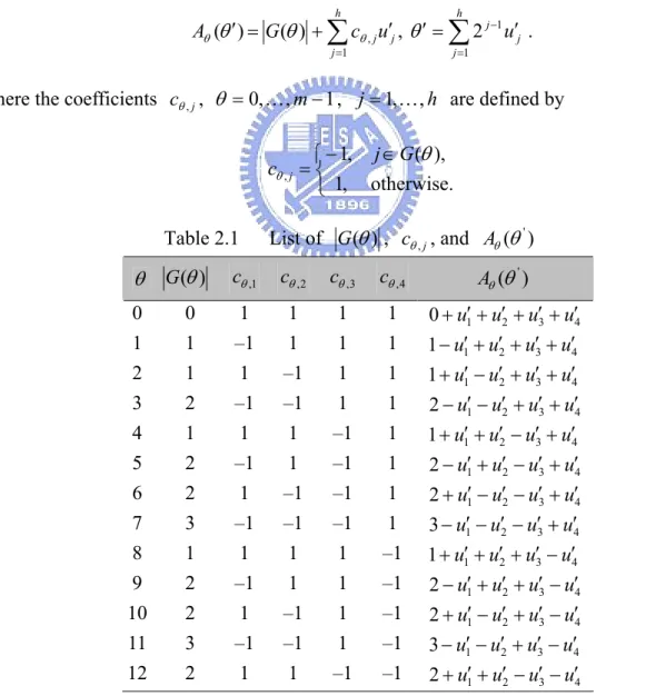
(19) function are equivalent with each other. Here, a general form of pressing a piecewise linear function by the existing methods, as in the textbook of Bazaraa et al. (1993), Floudas (2000), and Vajda (1964) or in the articles of Croxton et al. (2003), Li (1996), Li and Lu (2008), Padberg (2000), and Topaloglu and Powell (2003), are formulated below: First introducing m binary variables λ0 , λ1 ,K, λm−1 to express the inequalities: aθ − ( am − a0 )(1 − λθ ) ≤ x ≤ aθ +1 + ( am − a0 )(1 − λθ ), θ = 0,K, m − 1 ,. (2.1). where m −1. ∑ λθ = 1 , θ =0. λθ ∈ {0,1} .. (2.2). There is one and only one θ = k (over θ ∈ {0,K, m − 1} ), in which λ k = 1 . That means, only one interval [ak , ak +1 ] is activated, which results in ak ≤ x ≤ ak +1 . Following Expression (2.1), the piecewise linear function f ( x) can be expressed as:. f (aθ ) + sθ ( x − aθ ) − M (1 − λθ ) ≤ f ( x) ≤ f (aθ ) + sθ ( x − aθ ) + M (1 − λθ ), θ = 0,K, m − 1 (2.3) where M = max{ f (aθ ) + sθ (am − aθ ), f (aθ ) + sθ (a0 − aθ )} θ. − min{ f (aθ ) + sθ (a m − aθ ), f (aθ ) + sθ (a0 − aθ )}, θ. and sθ =. f ( aθ +1 ) − f ( aθ ) . aθ +1 − aθ. (2.4). REMARK 2.1 Expressing f (x) by (2.1) through (2.4) requires m binary variables. λ0 ,K, λm−1 and 4m constraints (i.e., inequalities (2.1) － (2.3)), where m + 1 is the number of break points.. 2.2 Superior Representation of Binary Variables (SRB) Let θ be an integer, 0 ≤ θ ≤ m − 1 , expressed as: 10.

(20) h. θ = ∑ 2 j −1 u j , h = ⎡log 2 m ⎤ , u j ∈ {0,1}.. (2.5). j =1. Given a θ ∈ {0, K , m − 1} , there is a unique set of {u j } meets (2.5). Let G (θ ) ⊆ {1,K, h} be the subset of indices such that:. ∑θ2. j −1. = θ.. (2.6). j∈G ( ). For instance, G (0) = φ , G (1) = {1} , G (2) = {2} , G (3) = {1,2} , etc. Let G (θ ) denote the number of elements in G (θ ) . For instance, G (0) = 0 , G (3) = 2 , etc. Define m functions Aθ (θ ′) (θ = 0,K, m − 1) based on a binary vector u′ = (u1′ , K , u h′ ) as follows: h. h. j =1. j =1. Aθ (θ ′) = G (θ ) + ∑ cθ , j u ′j , θ ′ = ∑ 2 j −1 u ′j .. (2.7). where the coefficients cθ , j , θ = 0, K , m − 1 , j = 1, K , h are defined by ⎧− 1, j ∈ G (θ ), cθ , j = ⎨ ⎩ 1, otherwise. Table 2.1. θ G (θ ) 0 1 2 3 4 5 6 7 8 9 10 11 12. 0 1 1 2 1 2 2 3 1 2 2 3 2. (2.8). List of G (θ ) , cθ , j , and Aθ (θ ' ). cθ ,1. cθ , 2. cθ ,3. cθ , 4. Aθ (θ ' ). 1 –1 1 –1 1 –1 1 –1 1 –1 1 –1 1. 1 1 –1 –1 1 1 –1 –1 1 1 –1 –1 1. 1 1 1 1 –1 –1 –1 –1 1 1 1 1 –1. 1 1 1 1 1 1 1 1 –1 –1 –1 –1 –1. 0 + u1′ + u2′ + u3′ + u4′ 1 − u1′ + u2′ + u3′ + u4′ 1 + u1′ − u2′ + u3′ + u4′ 2 − u1′ − u2′ + u3′ + u4′ 1 + u1′ + u2′ − u3′ + u4′ 2 − u1′ + u2′ − u3′ + u4′ 2 + u1′ − u2′ − u3′ + u4′ 3 − u1′ − u2′ − u3′ + u4′ 1 + u1′ + u2′ + u3′ − u4′ 2 − u1′ + u2′ + u3′ − u4′ 2 + u1′ − u2′ + u3′ − u4′ 3 − u1′ − u2′ + u3′ − u4′ 2 + u1′ + u2′ − u3′ − u4′. 11.

(21) For instance, given an arbitrary number m = 13, a list of all values of G (θ ) , cθ , j , and Aθ (θ ' ) for given θ are shown in Table 2.1. G (θ ) and cθ , j in (2.7) are not intuitive forms, then it can be rewritten more intuitive as follows. PROPOSITION 2.1. G (θ ) and cθ , j in (2.7) can be rewritten as follows: ⎢ θ ⎥ ⎢ j −1 ⎥ ⎦. h. G (θ ) = 0.5∑ (1 − (−1) ⎣ 2 j =1. cθ , j = (−1). ⎢ θ ⎥ ⎢ j −1 ⎥ ⎣2 ⎦. ) , θ = 0, K , m − 1 , h = ⎡log 2 m ⎤ ,. (2.9). , θ = 0, K , m − 1 , j = 1,..., ⎡log 2 m ⎤ .. (2.10). PROOF In (2.7), where cθ , j = −1 if j ∈ G (θ ) , otherwise cθ , j = 1 .. Obviously: cθ ,1 = ( −1). ⎢θ ⎥ ⎢1⎥ ⎣ ⎦. cθ , 2 = ( −1). ⎢θ ⎥ ⎢2⎥ ⎣ ⎦. = ( −1). ⎢θ ⎥ ⎢ 20 ⎥ ⎣ ⎦. = ( −1). ⎢θ ⎥ ⎢ 21 ⎥ ⎣ ⎦. M. cθ ,h = ( −1) G (θ ) =. ⎢ θ ⎥ ⎢ 2h −1 ⎥ ⎣ ⎦. (1 − cθ ,1 ) + (1 − cθ , 2 ) + ... + (1 − cθ , h ) 2. h. = 0.5∑ (1 − (−1). ⎢ θ ⎥ ⎢ h −1 ⎥ ⎣2 ⎦. ). j =1. This proposition is then proven.. □. Then we have following main theorem: THEOREM 2.1 For an integer θ in (2.5) and (2.6), given a binary vector u ' = (u1' ,K, uh' ) ,. there is one and only one k , 0 ≤ k ≤ m − 1 , such that. (i). Ak (θ ' ) = 0 if θ ' = k ,. 12.

(22) (ii). Ak (θ ' ) ≥ 1 , otherwise. h. PROOF There is one and only one k , such that k = ∑ 2 j −1 u j + 1 . j =1. (i). If k = θ ' that u 'j = u j ∀ j , which results in. ∑u. j∈G ( k ). ' j. =. ∑u. j∈G ( k ). j. ∑u. = G (k ) and. j∉G ( k ). =. ' j. ∑u. j∉G ( k ). j. = 0.. Thus to have Ak (θ ' ) = 0 . (ii). If k ≠ θ ' then. G (θ ) ≥. ∑u. j∈G ( k ). ' j. and. ∑u. j∉G ( k ). ' j. ≥ 1,. therefore Aθ (θ ' ) ≥ 1 .. □. For instance, given u ' = (u1' ,K, uh' ) = (0,1,0,1) in Table 2.1, we have A0 (θ ′) = G (0) + u1′ + u 2′ + u3′ + u 4′ + = 0 + 0 + 1 + 0 + 1 = 2 , A1 (θ ′) = G (1) − u1′ + u 2′ + u3′ + u 4′ + = 1 − 0 + 1 + 0 + 1 = 3 , M. A10 (θ ′) = G (10) + u1′ − u 2′ + u3′ − u 4′ + = 2 + 0 − 1 + 0 − 1 = 0 , A11 (θ ′) = G (11) − u1′ − u 2′ + u3′ − u 4′ + = 3 − 0 − 1 + 0 − 1 = 1 , A12 (θ ′) = G (12) + u1′ + u 2′ − u3′ − u 4′ + = 2 + 0 + 1 − 0 − 1 = 2 ,. Here A10 (θ ′) = 0 ; Aθ (θ ′) ≥ 0 for 0 ≤ θ ≤ 12 and θ ≠ 10 .. PROPOSITION 2.2. For a set of non-negative continuous variables ( r0 ,K, rm−1 ) , if m −1. ∑ rθ = 1 ,. θ =0. 13. (2.11).

(23) m −1. ∑ rθ Aθ (θ ′) = 0 ,. (2.12). θ =0. then the values of rθ , θ = 0,K, m − 1 , are either 0 or 1, where Aθ (θ ′) are defined by (2.6) －(2.8).. PROOF By referring to THEOREM 2.1, there is one and only one k , 0 ≤ k ≤ m − 1 , such that. Ak (θ ′) = 0. and. Aθ (θ ′) ≥ 1. for. 0 ≤ θ ≤ m −1. θ ≠ k . Since. and. rθ ≥ 0 ,. 0 ≤ θ ≤ m − 1, the only solution to satisfy (2.11) and (2.12) is rk = 1 and rθ = 0 for. θ ≠ k . The proposition is then proven.. □. Expression (2.12) is nonlinear and needs to be linearized. We have m −1. ∑ rθ Aθ (θ ′) θ =0. = r0 ( G (0) + c0,1u1′ + K + c0,h u h′ ) + K. (2.13) + rm−1 ( G (m − 1) + cm−1,1u1′ + K + cm−1,h u ′h ) m −1. m −1. m −1. θ =0. θ =0. θ =0. = ∑ rθ G (θ ) + u1′ ∑ rθ cθ ,1 + K + u h′ ∑ rθ cθ ,h = 0. Denote m −1. z j = u′j ∑ rθ cθ , j , ∀j. (2.14). θ =0. We then have following proposition:. PROPOSITION 2.3. The nonlinear expression. m −1. ∑ rθ Aθ (θ ′) = 0. in (2.12) can be replaced. θ =0. by the following linear system: m −1. h. =0. j =1. ∑ rθ G(θ ) + ∑ z θ 14. j. = 0,. (2.15).

(24) − u′j ≤ z j ≤ u′j , u′j ∈ {0,1}, j = 1,K, h , m −1. m −1. θ =0. θ =0. ∑ rθ cθ , j − (1 − u′j ) ≤ z j ≤ ∑ rθ cθ , j + (1 − u′j ), j = 1,K, h .. (2.16) (2.17). PROOF By referring to (2.14), (2.13) can be converted into (2.15). According to (2.8) and PROPOSITION 2.2 we have cθ , j ∈{1,−1} and. rθ ∈{0,1} , which cause − 1 ≤ z j ≤ 1 .. Expression (2.14) therefore can be linearized by (2.16) and (2.17). Two cases can be check for each u′j : (i). If u′j = 0 , then z j = 0 referring to (2.16),. (ii). If u ′j = 1 , then z j = ∑ rθ cθ , j referring to (2.17).. m −1. θ =0. m −1. Both (i) and (ii) imply that z j = u′j ∑ rθ cθ , j . Expression (2.14) can be replaced by θ =0. (2.15)－(2.17).. □. 2.3 The Proposed Linear Approximation Method Consider the same piecewise linear function f ( x ) described in Figure 2.1, where x is within the interval [a0 , am ] , and there are m + 1 break points a0 < a1 < K < am within [a0 , am ] . By referring to PROPOSITION 2.2 and PROPOSITION 2.3, f (x) with division of the interval [a0 , am ] into m subintervals can be expressed as: m −1. m −1. θ =0. θ =0. ∑ rθ aθ ≤ x ≤ ∑ rθ aθ +1 ,. f ( x). =. m −1. ∑ rθ ( f ( aθ ) + sθ ( x − a. θ =0. =. 0. (2.18). + a 0 − aθ )). m −1. m −1. θ =0. θ =0. ∑ ( f ( aθ ) − sθ ( aθ − a0 )) rθ + ∑ sθ rθ ( x − a0 ) 15. (2.19).

(25) where sθ are slopes of f ( x) as defined in (2.4). By referring to PROPOSITION 2.2, rθ ∈{0, 1} and (2.19). imply. that:. if. rθ ∑ θ. rk = 1, k ∈ {1,K, m − 1},. = 1 , Expressions (2.18) and. m −1. aθ rθ ( x − a ) ∑ θ. f ( x) = f (ak ) + sk ( x − ak ) . The nonlinear term. ak ≤ x ≤ ak +1. then. 1. =1. and. in (2.19) can then be. linearized as follows. Denote wθ = rθ ( x − a0 ) , since there is one and only one k , k ∈ {0,K, m − 1} such that rk = 1 and Ak (θ ′) = 0 , it is clear that: m −1. ∑ wθ = x − a. θ =0. 0. ,. (2.20). m −1. ∑ wθ Aθ (θ ′) = 0 .. (2.21). θ =0. By referring to (2.15), we then have. m −1. m −1. h. m −1. θ =0. θ =0. j =1. θ =0. ∑ wθ Aθ (θ ′) = ∑ wθ G(θ ) + ∑ u ′j (∑ wθ cθ , j ) = 0 .. m −1. Denote δ j = u′j ∑ wθ cθ , j for all j , the term θ =0. m −1. ∑ wθ Aθ (θ ′). can be expressed as below. θ =0. referring to PROPOSITION 2.2: m −1. h. θ =0. j =1. ∑ wθ G(θ ) + ∑ δ j = 0 ,. (2.22). − ( am − a0 )u′j ≤ δ j ≤ ( am − a0 )u′j , j = 1,K, h ,. (2.23). m −1. m −1. θ =0. θ =0. ∑ wθ cθ , j − (am − a0 )(1 − u′j ) ≤ δ j ≤ ∑ wθ cθ , j + (am − a0 )(1 − u′j ), j = 1,K, h .. (2.24). We then deduce our main result:. THEOREM 2.2. Let f ( x ) be a piecewise linear function defined in a given interval. x ∈ [a0 , am ] with m subintervals by m + 1 break points: a0 < a1 < K < am . f (x) can be expressed by the following linear system: 16.

(26) m −1. m −1. θ =0. θ =0. ∑ rθ aθ ≤ x ≤ ∑ rθ aθ +1 ,. (2.25). m −1. m −1. θ =0. θ =0. f ( x ) = ∑ ( f ( aθ ) − sθ ( aθ − a0 )) rθ + ∑ sθ wθ ,. (2.26). m −1. ∑ rθ = 1, rθ ≥ 0 ,. (2.27). θ =0 m −1. h. θ =0. j =1. ∑ rθ G(θ ) + ∑ z j = 0 ,. (2.28). − u′j ≤ z j ≤ u′j , j = 1,K, h ,. (2.29). m −1. m −1. θ =0. θ =0. ∑ rθ cθ , j − (1 − u′j ) ≤ z j ≤ ∑ rθ cθ , j + (1 − u′j ), j = 1,K, h ,. (2.30). m −1. ∑ wθ = x − a. θ =0. m −1. ∑ wθ cθ θ =0. m −1. h. θ =0. j =1. 0. ,. (2.31). ∑ wθ G(θ ) + ∑ δ j = 0 ,. (2.32). − ( am − a0 )u′j ≤ δ j ≤ ( am − a0 )u′j , j = 1,K, h ,. (2.33). m −1. ,j. − ( am − a0 )(1 − u′j ) ≤ δ j ≤ ∑ wθ cθ , j + ( am − a0 )(1 − u′j ), j = 1,K, h ,. (2.34). θ =0. h. ∑2 j =1. j −1. u ′j ≤ m .. (2.35). where (2.25) and (2.26) come from (2.18) and (2.19), (2.27) from (2.11), (2.28)－(2.30) from PROPOSITION 2.3, and (2.31)－(2.34) from (2.21)－(2.24).. REMARK 2.2 Expressing f (x) with m + 1 break points by THEOREM 2.2 uses ⎡log 2 m ⎤ binary variables, 8 + 8⎡log 2 m ⎤ constraints, 2m non-negative continuous variables, and 2 ⎡log 2 m ⎤ free-signed continuous variables. 17.

(27) Comparing REMARK 2.1 with REMARK 2.2 to know that, in expressing f (x) with large number of break points, the proposed method uses much less number of binary variables and constraints than being used in the existing methods.. 2.4 Numerical Examples EXAMPLE 2.1 Consider the following nonlinear programming problem:. P1 Min x1α1 − x2β1 s.t.. x1α 2 − 6 x1 + x2β 2 ≤ b, x1 + x2 ≤ 8, 1 ≤ x1 ≤ 7.4, 1 ≤ x2 ≤ 7.4 ,. where α1 , β1 , α 2 , β 2 and b are fixed constants. Various α1 , β1 , α 2 , β 2 and b values are specified in this experiment to compare the computational efficiency of expressing the piecewise linear functions by the existing method (i.e., (2.1)－(2.4)) and by our proposed method (i.e., THEOREM 2.2). For the first experiment given, α1 = 0.4 , β1 = 2 , α 2 = 1.85 , β 2 = 2 , b = 5 , the nonlinear terms x10.4 and − x22 are concave and required to be linearized, while the other convex terms x11.85 and x22 do not need linearization. Suppose m + 1 equal-distance break points are chosen to linearize each of x10.4 and − x22 , denoted as a0 = 1 , aθ = 1 + 6.4θ / m , am = 7.4 , for θ = 1,K, m − 1 . Then existing methods (i.e., (2.1)－(2.4)) require to use 2m binary variables and 8m extra constraints to piecewisely linearize x10.4 and − x22 . However, by piecewisely linearize the same convex terms, our proposed method (i.e., THEOREM 2.2) 18.

(28) only uses 2 ⎡log 2 m ⎤ binary variables, 14 + 16⎡log 2 m ⎤ extra constraints, 4m non-negative continuous variables, and 2 ⎡log 2 m ⎤ free-signed continuous variables. The linearization of x10.4 by the proposed method is described below: Denote f ( x1 ) = x10.4 . By THEOREM 2.2, f ( x1 ) with m = 64 is expressed by the following linear equations and inequalities: 63. 63. θ =0. θ =0. ∑ rθ aθ ≤ x1 ≤ ∑ rθ aθ +1 ,. 63. 63. θ =0. θ =0. f ( x1 ) = ∑ (aθ0.4 − sθ (aθ − a0 ))rθ + ∑ sθ wθ , 63. ∑ rθ. θ =0. 63. = 1, rθ ≥ 0 ,. ∑ wθ θ. = x −1,. =0. 63. 6. =0. j =1. ∑ rθ G(θ ) + ∑ z θ. j. =0,. − u ′j ≤ z j ≤ u ′j , j = 1, K ,6 , 63. 63. θ =0. θ =0. ∑ rθ cθ , j − (1 − u′j ) ≤ z j ≤ ∑ rθ cθ , j + (1 − u′j ), j = 1, K ,6 , 63. 6. θ =0. j =1. ∑ wθ G(θ ) + ∑ δ j = 0 ,. − 6.4u ′j ≤ δ j ≤ 6.4u ′j , j = 1, K ,6 , 63. 63. θ =0. θ =0. ∑ wθ cθ , j − 6.4(1 − u′j ) ≤ δ j ≤ ∑ wθ cθ , j + 6.4(1 − u′j ), j = 1, K ,6 ,. aθ0.+41 − aθ0.4 , u′j ∈ {0,1} , ∀j . where sθ = aθ +1 − aθ Similarly, − x 22 can be piecewisely linearized by THEOREM 2.2. The original program 19.

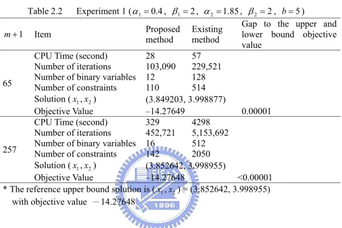
(29) is then converted into a mixed 0-1 convex program. We solve this program on LINGO (2004) by both the existing methods and the proposed method. The related solutions, CPU time, number of iterations, number of binary variables, number of constraints, and gap to the upper and lower bound objective value are listed in Table 2.2. Experiment 1 ( α 1 = 0.4 , β1 = 2 , α 2 = 1.85 , β 2 = 2 , b = 5 ) Gap to the upper and Proposed Existing m + 1 Item lower bound objective method method value CPU Time (second) 28 57 Number of iterations 103,090 229,521 Number of binary variables 12 128 65 Number of constraints 110 514 Solution ( x1 , x2 ) (3.849203, 3.998877) Objective Value –14.27649 0.00001 CPU Time (second) 329 4298 Number of iterations 452,721 5,153,692 Number of binary variables 16 512 257 Number of constraints 142 2050 Solution ( x1 , x2 ) (3.852642, 3.998955) Objective Value –14.27648 <0.00001 * The reference upper bound solution is ( x1 , x2 ) = (3.852642, 3.998955) with objective value －14.27648 Table 2.2. The gaps between the upper and lower bounds can be computed as follows. (i). Solve the nonlinear program P1 directly by a nonlinear optimization software (such as LINGO). The solution is x 0 = ( x10 , x20 ) = (3.852642, 3.998955) with objective value －14.27648. x 0 is one of the local optima of P1. But it is unknown about the gap. between x 0 and the global optimum. x 0 is regarded as the upper bound solution. (ii). Divide the ranges of both x1 and x2 into 65 break points. Let ( x10 , x20 ) replace the nearest break point (3.8, 4.0) in the existing 65 break points. Solving the program by both. the. proposed. method. and 20. the. existing. method. to. obtain.

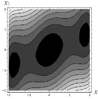
(30) x ∆ = (3.849203, 3.998877) with objective value －14.27649. x ∆ is a lower bound solution of P1. The gap between the objective values of x 0 and x ∆ is 0.00001. (iii) Reiterate to (ii), divide the ranges of both x1 and x2 into 257 break points. Solving the program by both methods to obtain the solution (3.852642, 3.998955), which is the same as x ∆ . Various combinations of α1 , β1 , α 2 , β 2 and b are specified to test the computation results of the existing methods and the proposed method. Parts of the results are displayed in Table 2.3. All these experiments demonstrate that the proposed method is much faster than the existing method especially when m becomes large.. EXAMPLE 2.2 This example, modified from Dixon and Szegö (1975), is to find the approximated global optimum of the following program:. P2 1 Min 2 x12 − 1.081x14 + x16 − x1 x2 + x22 + 0.01x1 6 s.t.. − 2 ≤ xi ≤ 2 , i = 1,2 ,. where the object function is a non-symmetrical three-humped camelback function. Figure 2.2 shows a contour map of this function under − 2 ≤ x1 ≤ 2 and − 2 ≤ x2 ≤ 2 . Here a reference upper bound solution is ( x1 , x2 ) = ( −1.802271,−0.9011357). with objective. value –0.02723789. For solving this program, let x1′ = x1 + 2.1 > 0 and x2′ = x2 + 2.1 > 0 to have x1 x2 = x1′ x2′ − 2.1x1′ − 2.1x2′ + 4.41 . Replace x1′ x′2 by exp( y ) , P2 then becomes P3 below: 21.

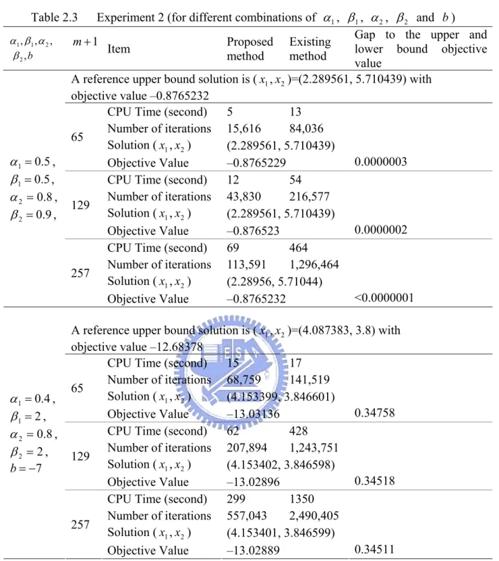
(31) Experiment 2 (for different combinations of α1 , β1 , α 2 , β 2 and b ) Gap to the upper and m +1 Proposed Existing Item lower bound objective method method value A reference upper bound solution is ( x1 , x2 )=(2.289561, 5.710439) with objective value –0.8765232 CPU Time (second) 5 13 Number of iterations 15,616 84,036 65 Solution ( x1 , x2 ) (2.289561, 5.710439) 0.0000003 Objective Value –0.8765229 CPU Time (second) 12 54 Number of iterations 43,830 216,577 129 Solution ( x1 , x2 ) (2.289561, 5.710439) 0.0000002 Objective Value –0.876523 CPU Time (second) 69 464 Number of iterations 113,591 1,296,464 257 Solution ( x1 , x2 ) (2.28956, 5.71044) <0.0000001 Objective Value –0.8765232. Table 2.3 α1 , β1 , α 2 , β2 , b. α 1 = 0 .5 , β 1 = 0 .5 , α 2 = 0 .8 , β 2 = 0 .9 ,. α 1 = 0 .4 , β1 = 2 , α 2 = 0 .8 , β2 = 2 , b = −7. A reference upper bound solution is ( x1 , x2 )=(4.087383, 3.8) with objective value –12.68378 CPU Time (second) 15 17 Number of iterations 68,759 141,519 65 Solution ( x1 , x2 ) (4.153399, 3.846601) 0.34758 Objective Value –13.03136 CPU Time (second) 62 428 Number of iterations 207,894 1,243,751 129 Solution ( x1 , x2 ) (4.153402, 3.846598) 0.34518 Objective Value –13.02896 CPU Time (second) 299 1350 Number of iterations 557,043 2,490,405 257 Solution ( x1 , x2 ) (4.153401, 3.846599) 0.34511 Objective Value –13.02889. 22.

(32) Figure 2.2. Contour map of the three-humped camelback function. P3 Min 2 x12 − 1.081x14 + s.t.. 1 6 x1 − exp( y ) + x22 + 2.11x1 + 2.1x2 + 4.41 6. y = ln x1′ + ln x2′ , x1 = x1′ − 2.1 , x2 = x2′ − 2.1 ,. − 2 ≤ xi ≤ 2 , i = 1,2 . The terms − x14 , − exp( y ) , ln x1′ and ln x′2 in P3 are non-convex, here we use − z1 , − z 2 , y1 and y2 to respectively as piecewise linear function to approximate those. non-convex terms. We then obtain the following mixed-integer program:. P4 1 Min 2 x12 − 1.081z1 + x16 − z 2 + x22 + 2.11x1 + 2.1x2 + 4.41 6. 23.

(33) s.t.. The same constraints as in P3, but replace ln x1′ and ln x2′ by y1 and y2 respectively.. We take 41 equal-distance break points for the value range of x1 and x2 ( [-2, 2] ), denoted as a0 = −2, a1 = −1.9 , a2 = −1.8,..., a40 = 2. It is clear that the break points for x1′ and x2′ are (0.1, 0.2,...,4.1) . Base on THEOREM 2.2, each of z1 , y1 , and y 2 is linearized with 6 binary variables and 55 constrains. Since y = y1 + y 2 , the region of y is [ln 0.1 + ln 0.1, ln 4.1 + ln 4.1]. = [ln 0.01, ln16.81] . We take m + 1 equal-distance break. points for the value range of y , denoted. as b0 = ln 0.01 , bθ = ln(0.01 + 16.8θ / m) ,. bm = ln 16.81 , for θ = 1,2,..., m − 1 . z2 = e y can then be piecewisely linearized under various y values. Problem P4 is converted into a mixed 0-1 convex program. We solve this program using LINGO (2004) with the existing methods and the proposed method. The related solutions, CPU time, number of iterations, number of binary variables, number of constraints, and gaps to the upper and lower bound objective values are reported in Table 2.4.. Table 2.4. Experiment result of Example 2.2 Proposed Existing Gap to the upper and lower m + 1 Item method method bound objective value CPU Time (second) 239 834 Number of iterations 2,387,868 3,675,444 Number of binary variables 17 112 33 Number of constraints 161 532 Solution ( x1 , x2 ) (–1.849207, –0.9925797) Objective Value –0.2269442 0.19970631 CPU Time (second) 882 2,277 Number of iterations 1,610,422 7,467,149 Number of binary variables 18 144 65 Number of constraints 169 660 Solution ( x1 , x2 ) (–1.7657, –0.8942029) Objective Value –0.08396288 0.05672499 * The reference upper bound solution is ( x1 , x2 ) = (–1.802271, –0.9011357) with objective value –0.02723789 24.

(34) EXAMPLE 2.3 This example is used to illustrate the process of solving discrete functions, consider following program: Min x13 − 1.8 x12.8 + 0.8 x 22.2 − x 22.1 + x30.5 − 3.5 x 40.8 − 0.3 x51.1 s.t.. x11.2 + x 20.8 ≤ 8 , x11.2 − x31.7 ≤ 2 , x 22.1 − x 14.7 ≥ 4.5 , x 40.8 − x50.96 ≥ −3 , x 22.2 − x51.1 ≥ −0.1 ,. where xi are discrete variables for all i , xi ∈{1, 1 + c, ..., 1 + mc} = {d 0 ,..., d m } , where c is the discreteness of xi , and m + 1 is the number of discrete points.. The existing method solves this example by linearizing a nonlinear function x α , x ∈ {d 0 ,..., d m } as m. x α = d 0α + ∑ λθ ( dθα − d 0α ), θ =1. m. λθ ≤ 1, λθ ∈ {0,1}, ∑ θ =1. where m binary variables are used. THEOREM 2.2 can be applied to solve a discrete function x α , x ∈ {d 0 ,..., d m } where f (x) in (2.26) is replaced by xα as m. x α = ∑ dθα rθ , θ =0. and all other constraints in (2.27) － (2.30) and (2.35) are kept as the same with 25.

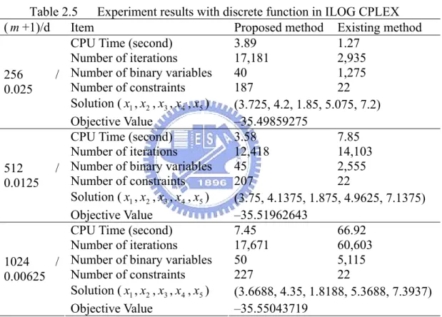
(35) θ = 0,..., m . For treating a discrete function, the proposed method uses log2 (m + 1) binary variables, 4 + 4⎡log2 (m + 1)⎤ constraints, m + 1 non-negative continuous variables, and. ⎡log 2 (m + 1)⎤ free-signed continuous variables. Table 2.5 is the computational result with ILOG CPLEX 9.0. It illustrates that the proposed method needs to use more constraints than the existing method; however, the proposed method is computationally more efficient then existing method for large m .. Table 2.5 Experiment results with discrete function in ILOG CPLEX ( m +1)/d Item Proposed method Existing method CPU Time (second) 3.89 1.27 Number of iterations 17,181 2,935 Number of binary variables 40 1,275 256 / Number of constraints 187 22 0.025 Solution ( x1 , x2 , x3 , x4 , x5 ) (3.725, 4.2, 1.85, 5.075, 7.2) Objective Value –35.49859275 CPU Time (second) 3.58 7.85 Number of iterations 12,418 14,103 Number of binary variables 45 2,555 512 / Number of constraints 207 22 0.0125 Solution ( x1 , x2 , x3 , x4 , x5 ) (3.75, 4.1375, 1.875, 4.9625, 7.1375) Objective Value –35.51962643 CPU Time (second) 7.45 66.92 Number of iterations 17,671 60,603 Number of binary variables 50 5,115 1024 / Number of constraints 227 22 0.00625 Solution ( x1 , x2 , x3 , x4 , x5 ) (3.6688, 4.35, 1.8188, 5.3688, 7.3937) Objective Value –35.55043719. 26.

(36) EXAMPLE 2.4 This example uses the same program in Example 2.3 but specifying all xi as continuous variables, where 1 ≤ xi ≤ 7.4 with m + 1 break points for all i . The comparison of the proposed method and the existing method, solving with ILOG CPLEX 9.0, is shown in Table 5. It demonstrates that the proposed method is also superior to the existing method for the continuous case.. Table 2.6. Experiment results with continuous function in ILOG CPLEX Proposed Existing Gap to the upper and lower m +1 Item bound objective value method method CPU Time (second) 4.23 39.86 Number of iterations 47,896 155,309 Number of binary variables 25 160 347 1,098 33 Number of constraints Solution ( x1 , x2 ) (3.67117699, 4.34398332) Solution ( x3 , x4 , x5 ) (1.8176404, 5.35913745, 7.4) Objective Value –35.56181842 0.00766842 CPU Time (second) 40.29 919.22 Number of iterations 250,747 1,437,056 Number of binary variables 30 320 407 2,186 65 Number of constraints Solution ( x1 , x2 ) (3.67115433, 4.34402387) Solution ( x3 , x4 , x5 ) (1.81765758, 5.3591112, 7.4) Objective Value –35.56160283 0.00745283 CPU Time (second) 454.21 4354.26 Number of iterations 2,128,203 8,690,141 Number of binary variables 35 640 Number of constraints 467 4,362 129 Solution ( x1 , x2 ) (3.67116282, 4.34402387) Solution ( x3 , x4 , x5 ) (1.81767335, 5.3591112, 7.4) Objective Value –35.56112235 0.00697235 * The reference upper bound solution is x1 = 3.668 , x2 = 4.352 , x3 = 1.816 , x4 = 5.373 , x5 = 7.4 with objective value –35.55415. 27.

(37) Chapter 3 Extension 1－Solving Generalized Geometric Programs Problems 3.1 3.2 3.3 3.4 3.5 3.6 3.7 3.8 3.9 3.10 3.11 3.12 3.13 3.14 3.15 3.16 3.17 3.18 3.19 3.20 3.21 3.22 3.23 Many optimization problems are formulated as Generalized Geometric Programming (GGP) containing signomial terms f (x) ⋅ g (y ) where x and y are continuous and discrete free-sign vectors respectively. By effectively convexifying f (x) and linearizing g (y ) , this chapter globally solves a GGP with less number of binary variables than are used in existing GGP methods. Numerical experiments demonstrate the computational efficiency of the proposed method.. 3.1 Introduction to Generalized Geometric Programming Generalized Geometric Programming (GGP) methods have been applied to solve problems in various fields, such as heat exchanger network design (Duffin and Peterson 1966), capital investment (Hellinckx and Rijckaert 1971), optimal design of cooling towers (Ecker and Wiebking 1978), batch plant modeling (Salomone and Iribarren 1992), competence sets expansion (Li 1999), smoothing splines (Cheng et al. 2005), and digital circuit (Boyd 2005). These GGP problems often contain continuous and discrete functions where the discrete variables may represent the sizes of components, thicknesses of steel plates, diameters of pipes, lengths of springs, and elements in a competence set etc. Many local optimization algorithms for solving GGP problems have been developed, which include linearization method (Duffin 1970), separable programming (Kochenberger et al. 1973), and a concave simplex algorithm (Beck and Ecker 1975). Pardalos and Romeijn (2002) provided an impressive overview of these GGP algorithms. Among existing GGP algorithms, the techniques developed by Maranas and Floudas (1997), Floudas et al. (1999), Floudas (2000) (these three methods are called Floudas’s methods in this study) are the most popular approaches for solving GGP problems. Floudas’s methods, however, can not be applied to 28.

(38) treat non-positive variables and discrete functions. Recently, Li and Tsai (2005) developed another method to modify Floudas’s methods thus to treat continuous variables containing zero values; however, Li and Tsai’s method is incapable of effectively handling mixed-integer variables. This study proposes a novel method to globally solve a GGP program with mixed integer free-sign variables. A free-sign variable is one which can be positive, negative, or zero. The GGP program discussed in this study is expressed below:. GGP Min. T0. ∑f p =1. s.t.. p. ( x) ⋅ G p ( y ). Tw. ∑f q =1. w ,q. ( x ) ⋅ G w,q ( y ) ≤ l w , w = 1,..., s ,. where n. (C1) f p ( x ) = c p ⋅ ∏ xi. α p ,i. i =1. n. , p = 1,..., T0 ,. (C2) f w,q ( x ) = hw,q ⋅ ∏ x i w , q ,i , w = 1,..., s , q = 1,..., Tw , α. i =1. m. (C3) G p ( y ) = ∏ g p , j ( y j ) , p = 1,..., T0 , j =1. m. (C4) G w,q (y ) = ∏ g w,q , j ( y j ) , w = 1,..., s , q = 1,..., Tw , j =1. (C5) x = ( x1 ,..., x n ) , is a vector with free-sign continuous variables xi , where xi can be positive, negative, or zero, x i ≤ xi ≤ xi , x i and xi are constants, (C6) y = ( y1 ,..., y m ) , is a vector with free-sign discrete variables y j , y j ∈ {d j ,1 ,..., d j ,rj } where d j , k can be positive, negative, or zero, (C7) g p , j ( y j ) and g w, q , j ( y j ) are nonlinear functions of y j , 29.

(39) (C8) α p ,i , α w,q ,i , c p , hw,q , and l w are constants, (C9) α p,i and α w,q ,i are integers if the lower bounds of xi are negative. Floudas’s method can solve a specific GGP problem containing continuous functions with positive variables, as illustrated below:. GGP1 (with continuous functions and positive variables) Min. T0. ∑f p =1. s.t.. p. (x). Tw. ∑f q =1. w,q. ( x ) ≤ l w , w = 1,..., s , x = ( x1 ,..., x n ) , x i ≤ xi ≤ xi , ∀ x i > 0 ,. where conditions (C1) and (C2) in GGP hold. For solving GGP1, Floudas’s method denotes xi = et i with ti = ln xi and group all monomials with identical sign. GGP1 is rewritten by Floudas’s method as follows: Min f 0+ ( t ) − f 0− ( t ) s.t.. f w+ ( t ) − f w− ( t ) ≤ l w , w = 1,..., s , f 0+ ( t ) = f 0− ( t ) =. ∑c. c p >0. p. ⋅e. ∑− c. c p <0. p. hp ( t). ⋅e. ,. hp ( t ). ,. h p ( t ) = ∑ α p ,i ⋅ ti , ∀p ,. (3.1). i. f w+ ( t ) =. ∑h. w ,q. ⋅e. hw , q ( t ). ,. hw , q > 0. f w− ( t ) =. ∑− h. hw , q < 0. w ,q. ⋅e. hw , q ( t ). ,. hw,q ( t ) = ∑ α w,q ,i ⋅ ti , ∀w, q . i. GGP1 is a signomial geometric program containing posynomial functions f 0+ ( t ) , 30.

(40) f w+ (t ) and signomial functions − f 0− ( t ) , − f w− (t ) where t = (t1 ,..., t n ) is a positive variable vector. A posynomial term is a monomial with positive coefficient, while a signomial term is a monomial with negative coefficient (Bazaraa et el. 1993; Floudas 2000). Supports all signomial terms in GGP1 are removed then we have a posynomial geometric program below: Min f 0+ ( t ) s.t.. f w+ ( t ) ≤ l w , w = 1,..., s .. Posynomial geometric program laid the foundation for the theory of generalized geometric program. Duffin and Peterson (1966) pioneered the initial work on posynomial geometric programs, which derived the dual based on the arithmetic geometric inequality. This dual involves the maximization of a separable concave function subject to linear constraints. Unlike posynomial geometric problems, signomial geometric problems remain nonconvex and much more difficult to solve. Floudas's method employs an exponential variable transformation to the initial signomial geometric program to reduce it into a decomposition program. A convex relaxation is then obtained based on the linear lower bounding of the concave parts. Floudas's method can reach ε-convergence to the global minimum by successively refining a convex relaxation of a series of nonlinear convex optimization problems. The ε − convergence to the global minimum ( ε − global minimum), as defined in Floudas (2000, page 58) is stated below: Suppose that x * is a feasible solution,. ε ≥ 0 is a small predescribed tolerance, and f ( x ) ≥ f (x * ) − ε for all feasible x , then x * is an ε − global minimum. However, the usefulness of Floudas's method is limited by the difficulty that xi must be strictly positive. This restriction prohibits many applications where xi can be zero or negative values (such as temperature, growth rate, etc.). In order to overcome the difficulty of Floudas’s methods, recently, Li and Tsai (2005) proposed another method for solving GGP1 where xi may be negative or zero. Li and Tsai 31.

(41) n. ∏ xi. first transfer. α p ,i. n. and. i =1. ∏x. α w , q ,i. into convex and concave functions, then approximate. i. i =1. the concave functions by piecewise linear techniques. Li and Tsai’s method can also reach finite ε-convergence to the global minimum. Both Floudas’s methods and Li & Tsai’s method use the exponential-based decomposition technique to decompose the objective function and constraints into convex and concave functions. Decomposition programs have good properties for finding a global optimum (Horst and Tuy, 1996). A convex relaxation of the decomposition can be computed conveniently based on the linear lower bound of the concave parts of the objective functions and constraints. Two difficulties of direct application of Floudas’s method or Li & Tsai method to globally solve a GGP problem are discussed below: (i). The major difficulty is that r − 1 binary variables are used in expressing a discrete variable. with. r. values.. For. instance,. to. linearize. a. signomial. term. G ( y ) = g1 ( y1 ) ⋅ g 2 ( y 2 ) = y1α1 ⋅ y 2α 2 where y j ∈ {d j ,1 , d j , 2 ,..., d j ,rj }∀j , rj , by taking the logarithm of G ( y ) one obtains 2. rj. j =1. k =2. ln G ( y ) = α1 ln y1 + α 2 ln y 2 = ∑ α j [ln d j ,1 + ∑ u j ,k (ln d j ,k − ln d j ,k −1 )] rj. where. ∑u k =2. j ,k. ≤ 1, u j ,k ∈ {0,1} .. It require r1 + r2 − 2 binary variables to linearly decompose G ( y ) . If the number of r j is large then it will cause a heavy computational burden. (ii). Another difficulty is the treatment of taking logarithms of y j . If y j may take on a negative or zero value then we can not take logarithmic directly. 32.

(42) This study proposes a novel method to globally solve GGP programs. The advantages of the proposed method are listed as below: Less number of binary variables and constraints are used in solving a GGP program. Only m. ∑ ⎡log r ⎤ 2. r =1. j. binary variables are required to linearize g p , j ( y j ) and g w,q , j ( y j ) in GGP. It. is capable of treating non-positive variables in the discrete and continuous functions in GGP. This study is organized as follows. Section 3.2 develops the first approach of treating discrete functions in GGP. Section 3.3 describes another approach of treating discrete functions. Section 3.4 proposes a method for handling continuous functions. Numerical examples are analyzed in Section 3.5.. 3.2 The Proposed Linear Approximation Method Form the basic of THEOREM 2.1, we develop two approaches to express a discrete variable y with r values. The first approach, as described in this section, use ⎡log 2 r ⎤ binary variables and 2r extra constraints to express y . The second approach, as described in the next section, use ⎡log 2 r ⎤ binary variables but only 3 + 4⎡log 2 r ⎤ constraints to express m. y . The first approach is good at treating product terms f ( x )∏ g j ( y j ) , while the second j =1. approach is more effective in treating additive terms. ∑g. j. (yj ) .. j. REMARK 3.1 A discrete free-sign variable y, y ∈ {d1 , d 2 ,..., d r } can be expressed as: d k − M ⋅ Ak ≤ y ≤ d k + M ⋅ Ak , k = 1,..., r where 33. (3.2).

(43) in (2.5) and Ak is same as Aθ (θ ′) in (2.7).. (i). k is same as θ. (ii). M is a big enough positive value, M = max{1, d1 ,..., d r } − min{0, d1 ,..., d r } .. (3.3). PROOF (i) If Ak = 0 then y = d k , (ii) If Ak ≥ 1 then d k − M ⋅ Ak ≤ min{0, d1 ,..., d r } ≤ y ≤ max{0, d1 ,..., d r } ≤ d k + M ⋅ Ak . Therefore (3.2) is still correct.. □. Take Table 2.1 for instance, for y ∈ {−1, 0, 1, 4, 5, 6, 7.5, 8, 9, 10} , y can be expressed by linear inequalities below:. − 1 − M (0 + u1′ + u 2′ + u3′ + u 4′ ) ≤ y ≤ −1 + M (0 + u1′ + u 2′ + u3′ + u 4′ ) , 0 − M( 1 − u1′ + u 2′ + u3′ + u 4′ ) ≤ y ≤ 0 + M( 1 − u1′ + u 2′ + u3′ + u ′4 ) , M. 10 − M( 2 − u1′ + u 2′ + u3′ − u 4′ ) ≤ y ≤ 10 + M( 2 − u1′ + u 2′ + u3′ − u ′4 ) , where M = 10 + 1 = 11 . In this case r = 10 and there are 2 × 10 = 20 constraints being used to express y . Since depending on the final u1′ , u 2′ , u3′ , and u ′4 assignments, only two of 20 inequalities will turn into equalities which indicate the discrete choice made of y , while the rest of 18 inequalities turn into redundant constraints.. REMARK 3.2 Expression (3.2) uses ⎡log 2 r ⎤ binary variables and 2r constraints to express a discrete variable with r values.. 34.

(44) Given a function g ( y ) where y ∈ {d1 , d 2 ,..., d r }, d k are discrete. PROPOSITION 3.1. free-sign values, g ( y ) can be expressed by following linear inequalities: g (d k ) − M ⋅ Ak ≤ g ( y ) ≤ g (d k ) + M ⋅ Ak , k = 1,..., r where y , Ak ,and k are specified in REMARK 3.1, and M = max{1, g (d1 ),..., g (d r )} − min{0, g (d1 ),..., g (d r )} .. (3.4). n. A product term z = f ( x ) ⋅ g ( y ) , where f ( x ) = c∏ xiαi. PROPOSITION 3.2. as being. i =1. specified in GGP, x i ≤ xi ≤ xi , c is a free-sign constant, and y ∈{d1 ,..., d r } , can be expressed by following inequalities: f ( x ) ⋅ g (d k ) − M ′ ⋅ Ak ≤ z ≤ f ( x ) ⋅ g ( d k ) + M ′ ⋅ Ak , k = 1,..., r where (i). y , Ak ,and k are specified in PROPOSITION 3.1.. (ii). M ′ = f (x ) ⋅ M , for n. f ( x ) = max{1, | c | ∏ xiU } , where xiU = max{| xiα i |, x i ≤ xi ≤ xi ∀i} .. (3.5). i =1. PROOF It. is. clear. that. M ′ ≥ M | f (x ) |. for. x i ≤ xi ≤ xi .. Since. − M ′Ak ≤ − Mf ( x ) Ak and M ′Ak ≥ Mf ( x ) Ak . Two cases are discussed. (i). Case 1 for f ( x ) ≥ 0 . From Proposition 3 to have. f ( x ) ⋅ g (d k ) − Mf ( x ) ⋅ Ak ≤ f ( x ) g ( y ) ≤ f (x ) ⋅ g ( d k ) + Mf ( x ) ⋅ Ak . We then have. f ( x ) g ( d k ) − M ′ ⋅ Ak ≤ f ( x ) g ( y ) ≤ f ( x ) g ( d k ) + M ′ ⋅ Ak . (ii). Case 2 for f ( x ) < 0 . From Proposition 3 to have 35. Ak ≥ 0 ,.

(45) f ( x ) ⋅ g (d k ) − Mf ( x ) ⋅ Ak ≥ f ( x ) g ( y ) ≥ f (x ) ⋅ g ( d k ) + Mf ( x ) ⋅ Ak . Similar to Case 1, it is clear that. f ( x ) g ( d k ) − M ′ ⋅ Ak ≤ f ( x ) g ( y ) ≤ f ( x ) g ( d k ) + M ′ ⋅ Ak . The proposition is then proven.. □. REMARK 3.3 For a constraint z = f (x ) ⋅ g ( y ) ≤ a where a is constant, f ( x ) and g ( y ) are the same as in PROPOSITION 3.2. The constraint z ≤ a can be expressed by following inequalities:. f ( x ) ⋅ g ( d k ) − M ′ ⋅ A k ≤ a , k = 1,..., r , where M ′ is same in PROPOSITION 3.2. There are r constraints used to describe z ≤ a ; where only one of the constraints is activated(i.e., A k = 0 ) which indicates the discrete choice made by y , while the rest of r − 1 inequalities turn into redundant constraints.. We then deduce the main result below: σ. THEOREM 3.1 Denote z1 = f ( x ) ⋅ g1 ( y1 ) and zσ = zσ −1 ⋅ gσ ( yσ ) = f ( x ) ⋅ ∏ g j ( y j ) for j =1. n. σ = 2,..., m where f ( x ) = c∏ xiα , xi ≤ xi ≤ xi , c is a free-sign constant, and y j are i. i =1. discrete free-sign variables, y j ∈ {d j ,1 , d j , 2 ,..., d j ,rj } . The terms z1 , z 2 ,..., z m can be expressed by the following inequalities: (C1). f ( x ) ⋅ g1 ( d 1,k ) − M 1′ ⋅ A1,k ≤ z1 ≤ f ( x ) ⋅ g1 ( d 1,k ) + M 1′ ⋅ A1,k. (C2) z1 ⋅ g 2 (d 2,k ) − M 2′ ⋅ A 2,k ≤ z 2 ≤ z1 ⋅ g 2 (d 2,k ) + M 2′ ⋅ A 2,k …. 36. , k = 1,..., r1 , , k = 1,..., r2 ,.

(46) (Cm) z m−1 ⋅ g m (d m,k ) − M m′ ⋅ A m,k ≤ z m ≤ z m−1 ⋅ g m (d m,k ) + M m′ ⋅ A m,k. , k = 1,..., rm .. where (i). d j ,k − M j ⋅ A j ,k ≤ y j ≤ d j ,k + M j ⋅ A j ,k , j = 1,..., m , k = 1,..., r j ,. (ii). A j ,k = 0.5∑ (1 − ( −1) ⎣ 2. ⎢ k −1 ⎥ ⎢ w −1 ⎥ ⎦. θ. w =1. (iii) k = 1 +. ⎡log 2 r j ⎤. ∑2. w −1. w=1. θ. ⎢ k −1 ⎥ ⎢ w −1 ⎥ ⎦. ) + ∑ (( −1) ⎣ 2 w =1. ⋅ u j ,w ) , θ = 1,..., ⎡log 2 rj ⎤ for all j , k ,. u j ,w ≤ r j ,. j. (iv). M ′j = f ( x ) ⋅ ∏ σ i , f ( x ) is specified in (3.5), i =1. σ i = max{1, g i (di , k )} − min{0, gi (di , k )} , (3.6) k. k. j = 1,..., m, k = 1,..., rj .. PROOF (i) Consider (C1). Since M 1′ ≥ M ′ ≥ M = σ 1 , where M ′ and M are specified in PROPOSITION 3.2, (C1) is ture. (ii) If. Consider (C2). It is clear M 2′ = f(x) ⋅ σ1σ 2 . f ( x ) ≥ 0 then. z1 ⋅ g 2 ( d 2,k ) − M 2′ ⋅ A2,k ≤ z1 ⋅ g 2 ( d 2,k ) − f ( x )σ 1σ 2 ⋅ A2,k ≤ z1 ⋅ g 2 ( d 2,k ). and z1 ⋅ g 2 ( d 2,k ) ≤ z1 ⋅ g 2 ( d 2,k ) + f ( x )σ 1σ 2 ⋅ A2,k ≤ z1 ⋅ g 2 ( d 2,k ) + M 2′ ⋅ A2,k . If f ( x ) < 0 z1 ⋅ g 2 ( d 2,k ) + M 2′ ⋅ A2,k ≥ z1 ⋅ g 2 ( d 2,k ) − f ( x )σ 1σ 2 ⋅ A2,k ≥ z1 ⋅ g 2 ( d 2,k ) and z1 ⋅ g 2 ( d 2,k ) ≥ z1 ⋅ g 2 ( d 2,k ) + f ( x )σ 1σ 2 ⋅ A2,k ≥ z1 ⋅ g 2 ( d 2,k ) − M 2′ ⋅ A2,k . We then have z1 ⋅ g 2 (d 2,k ) − M 2′ ⋅ A2,k ≤ z 2 ≤ z1 ⋅ g 2 (d 2,k ) + M 2′ ⋅ A2,k for A2,k ≥ 1 . (iii) Similar for (C3) to (Cm). The theorem is then proven.. □. 37.

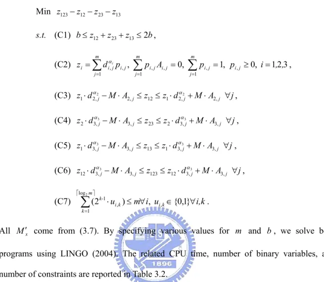
(47) REMARK 3.4 A n. Constraint. p. m. s =1. j =1. ∑ f s ( x )∏ g s , j ( y i ) ≤ a. ,. where. a. is. constant. and f s ( x ) = c s ∏ xi i , s , x i ≤ xi ≤ xi , c is a free-sign constant, can be expressed by α. i =1. following inequalities: p. ∑z s =1. s ,m. ≤ a,. z s ,m −1 ⋅ g s ,m ( d m,k ) − M s ,m ⋅ As ,m,k ≤ z s ,m ∀s, k , z s ,m −2 ⋅ g s ,m −1 ( d m −1,k ) − M s ,m −1 ⋅ As ,m −1,k ≤ z s ,m −1 ≤ z s ,m −2 ⋅ g s ,m −1 ( d m −1,k ) + M s ,m −1 ⋅ As ,m −1,k ∀s, k , M. z s , 2 ⋅ g s , 2 ( d 2,k ) − M s , 2 ⋅ As , 2,k ≤ z s , 2 ≤ z s ,2 ⋅ g s , 2 ( d 2,k ) + M s , 2 ⋅ As , 2,k ∀s, k , f s ( X ) ⋅ g s ,1 ( d 1,k ) − M s ,1 ⋅ As ,1,k ≤ z s ,1 ≤ f s ( X ) ⋅ g s ,1 ( d 1,k ) + M s ,1 ⋅ As ,1,k ∀s, k , where i. n. j =1. i =1. M s ,i = f s ( x ) ⋅ ∏ σ s ,i , f s ( x ) = max{1, | C s | ∏ x Us ,i }, x Us ,i = max{| xi s ,i |, x i ≤ xi ≤ xi }∀s, i, α. (3.7). σ s ,i = max{1, g s ,i (d i ,k )} − min{0, g s ,i (d i ,k )}.. For instance, a single nonlinear constraint xy12 + y1 y 2 ≤ a where 0 ≤ x ≤ 5 , y1 , y 2 are integer variables, 1 ≤ y1 , y 2 ≤ 32 , can be converted into a linear system as follows. (i). Denote. y1 ∈{1,...,32} = {d1 ,..., d 32 } . Since ⎡log 2 32⎤ = 5 , five binary variables. u1 , u 2 , u3 , u 4 , and u5 are used to express y1 . Specifying k as: k = 1 + u1 + 2u 2 + 2 2 u3 + 2 3 u 4 + 2 4 u5 . Referring to (3.2), y1 is expressed as d k − M 1 ⋅ A1,k ≤ y1 ≤ d k + M 1 ⋅ A1,k , k = 1,...,32, 38. (3.8).

(48) where M 1 = 32 and A1,k are specified as A1,1 = u1 + u 2 + u3 + u 4 + u 5 , A1, 2 = 1 − u1 + u 2 + u3 + u 4 + u 5 , M A1,32 = 5 − u1 − u 2 − u3 − u 4 − u5 .. Similarly, denote y 2 ∈ {1,...,32} = {b1 ,..., b32 } , five binary variables v1 , v2 , v3 , v4 , and v5 are used to express y2 . Specifying q as: q = 1 + v1 + 2v2 + 2 2 v3 + 23 v4 + 2 4 v5 . y2 is expressed in the same way as in y1 :. bq − M 2 ⋅ A2,q ≤ y 2 ≤ bq + M 2 ⋅ A2,q , q = 1,...,32,. (3.9). where M 2 = 32 . Specifying A2,q as A2,1 = v1 + v2 + v3 + v4 + v5 , A2, 2 = 1 − v1 + v2 + v3 + v4 + v5 , M A2,32 = 5 − v1 − v2 − v3 − v4 − v5 .. (ii). Treating the first term xy12 in the constraint. Denote z3 = xy12 . From Theorem 1 to have: x ⋅ d k2 − M 1′ ⋅ A1,k ≤ z3 , k = 1,...,32,. where M& 1 = 5 * (32 2 − 0) = 5120 (iii) The second term y1 y2 in constraint is treated similarly. Denote z4 = y1 y2 . To form. 39.

(49) the inequalities as y1 ⋅ bq − M 2′ ⋅ A2,q ≤ z 4 , q = 1,...,32, where M& 2 = 32 * 32 = 1024.. The original constraint then becomes z3 + z 4 ≤ a where there are additional 10 binary variables and two continuous variables. By utilizing Theorem 1 to express this constraint in linear form requires 192 additive constraints (where 64 come from (3.8), 64 come from (3.9)). Another approach, developed based on Theorem 1, can be used to reduce the number of constraints from 192 to 64 + 2(3 + 4⎡log 2 32⎤) = 110 .. 3.3 Treatment of Discrete Function in GGP (Approach 2) PROPOSITION 3.1 uses ⎡log 2 r ⎤ binary variables and 2r additive constraints to express a discrete function g ( y ) variable with r values. Here we use PROPOSITION 2.2 and PROPOSITION 2.3 to express the same discrete variable where only 3 + 4⎡log 2 r ⎤ additive constraints are required. Such an expression is computationally more efficient to treat g ( y ) in a GGP program. We use pk and δ w to instead of rθ and z j in PROPOSITION 2.2 and PROPOSITION 2.3 in this section respectively. For instance, given y ∈ {−1, 0, 1, 4, 5, 6, 7.5, 8, 9, 10} , referring to Table 2.1 to have. 40.

(50) 10. ∑p k =1. k. Ak = p1 (u1 + u2 + u3 + u4 ) + p2 (1 − u1 + u2 + u3 + u4 ) + ... + p10 ( 2 − u1 + u2 + u3 − u4 ) = u1 ( p1 − p2 + p3 − p4 + p5 − p6 + p7 − p8 + p9 − p10 ) + u2 ( p1 + p2 − p3 − p4 + p5 + p6 − p7 − p8 + p9 + p10 ) + u3 ( p1 + p2 + p3 + p4 − p5 − p6 − p7 − p8 + p9 + p10 ) + u4 ( p1 + p2 + p3 + p4 + p5 + p6 + p7 + p8 − p9 − p10 ) = 0.. The discrete variable y can be expressed by following linear equation and linear inequalities: y = − p1 + p3 + 4 p4 + 5 p5 + 6 p6 + 7.5 p7 + 8 p8 + 9 p9 + 10 p10 ,. δ 1 + δ 2 + δ 3 + δ 4 + p2 + p3 + ... + 2 p10 = 0, − u w ≤ δ w ≤ u w , w = 1,...,4, p1 − p2 + p3 − ... − p10 − 1 + u1 ≤ δ 1 ≤ p1 − p2 + p3 − ... − p10 + 1 − u1 , (3.10) p1 + p2 − p3 − ... − p10 − 1 + u 2 ≤ δ 2 ≤ p1 + p2 − p3 − ... − p10 + 1 − u 2 , M. p1 + p2 + p3 + ... − p10 − 1 + u 4 ≤ δ 4 ≤ p1 + p2 + p3 + ... − p10 + 1 − u 4 , 10. ∑p k =1. k. = 1, pk ≥ 0.. It is convenient to check: If u 2 = 1 and u1 = u3 = u 4 = 0 then δ 1 = δ 3 = δ 4 = 0 and. δ 2 = p1 + p2 − p3 − p4 + p5 + p6 − p7 − p8 + p9 + p10 . Since δ 2 + p2 + p3 + 2 p4 + p5 + 2 p6 + 2 p7 + 3 p8 + p9 + 2 p10 = p1 + 2 p2 + p4 + 2 p5 + 3 p6 + p7 + 2 p8 + 2 p9 + 3 p10 = 10 , pk ≥ 0 , and. 10. ∑p k =1. k. = 1 , it is clear. p1 = p2 = p4 = p5 = p6 = p7 = p8 = p9 = p10 = 0 , δ 2 + p3 = 0 , δ 2 = −1 and p3 = 1 . We 41.

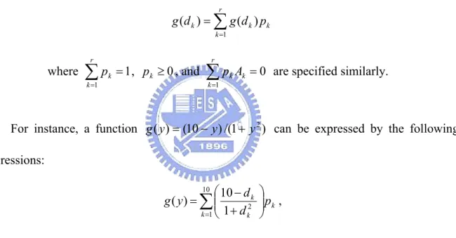
(51) then have y = p3 = 1 .. REMARK 3.5 ⎡log 2 r ⎤. binary variables, 3 + 4⎡log 2 r ⎤. constraints, and. r + ⎡log 2 r ⎤. continuous variables are used in PROPOSITION 2.2 and PROPOSITION 2.3 to express a discrete variable with r values.. REMARK 3.6 Given a function g ( y ) where y ∈{d1 ,..., d r } , g ( y ) can be expressed by following expressions. r. g ( d k ) = ∑ g ( d k ) pk k =1. where. r. ∑ pk = 1, pk ≥ 0 , and k =1. r. ∑p k =1. k. Ak = 0 are specified similarly.. For instance, a function g ( y ) = (10 − y ) /(1 + y 2 ) can be expressed by the following expressions: 10 ⎛ 10 − d k g ( y ) = ∑ ⎜⎜ 2 k =1 ⎝ 1 + d k. ⎞ ⎟⎟ pk , ⎠. Suppose u 2 = u3 = u 4 = 0 and u1 = 1 then k = 2, p2 = 1, y = 0 and g ( y ) = 10 .. Table 3.1 is a comparison of the three ways for expressing a discrete variable y with. r values. A numerical example is given in Example 3.4 to compare their computational effeciency.. 42.

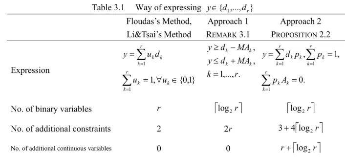
(52) Way of expressing y ∈{d1 ,..., d r }. Table 3.1. Floudas’s Method, Li&Tsai’s Method. Approach 1 REMARK 3.1 y ≥ d k − MAk ,. r. y = ∑ uk d k. y ≤ d k + MAk ,. k =1. Expression. r. ∑u k =1. k. = 1, ∀uk ∈ {0,1}. k = 1,..., r.. Approach 2 PROPOSITION 2.2 r. r. k =1. k =1. y = ∑ d k pk , ∑ pk = 1, r. ∑p k =1. k. Ak = 0.. No. of binary variables. r. ⎡log 2 r ⎤. ⎡log 2 r ⎤. No. of additional constraints. 2. 2r. 3 + 4⎡log 2 r ⎤. No. of additional continuous variables. 0. 0. r + ⎡log 2 r ⎤. Now consider Condition (i) in THEOREM 3.1, where y j are expressed by Approach 1 using 2r j constraints. That condition can be replaced by PROPOSITION 2.2 and PROPOSITION 2.3 where only 3 + 4⎡log 2 r ⎤ constraints are required. This is described as following proposition:. PROPOSITION 3.3. Replacing Condition (i) in THEOREM 3.1 by following expressions: rj. y j = ∑ d j ,k p j ,k , j = 1,..., m k =1. rj. where. ∑p k =1. j ,k. = 1 , p j ,k ≥ 0 , and. rj. ∑p k =1. j ,k. A j ,k = 0 for all j, k . The total number of. variables and constraints used to express y, z1 ,..., z m using (C1), (C2),…,(Cm) in THEOREM 3.1 are listed below: (i). no. of binary variables:. m. ∑ ⎡log r ⎤ , 2. j =1. (ii). j. m. no. of constraints for g j ( y j ) : 3m + ∑ ⎡log 2 r j ⎤ , j =1. m. (iii) no. of constraints for z1 , z 2 ,..., z m in (C1), (C2),…,(Cm): 4∑ r j , j =1. (iv) no. of continuous variables:. m. m. ∑ (r j =1. j. + 1) + ∑ ⎡log 2 r j ⎤ . j =1. 43.