整合繞徑法與擁塞控制改善廣域的公平性

全文

(1)國立交通大學電信工程學系碩士論文整合繞徑法與擁塞控制改善廣域的公平性 Unified Routing and Congestion control for Global Fairness 研究生：陳俊宏指導教授：廖維國. 教授. 中華民國九十七年四月.

(2) 整合繞徑法與擁塞控制改善廣域的公平性 Unified Routing and Congestion Control for Global Fairness 研究生：陳俊宏. Student：Chun-Hung Chen. 指導教授：廖維國. Advisor：Wei-Kuo Liao 國立交通大學電信工程學系碩士論文. A Thesis Submitted to Department of Communication Engineering College of Electrical and Computer Engineering National Chiao Tung University in partial Fulfillment of the Requirements for the Degree of Master in Communication Engineering. April 2008. Hsinchu, Taiwan, Republic of China. 中華民國九十七年四月.

(3) 整合繞徑法與擁塞控制改善廣域的公平性. 研究生︰陳俊宏. 指導教授︰廖維國博士. 國立交通大學電信工程學系. 摘要在我們的這篇研究中，考慮的情形是在當使用者在傳送資料的時候有多種選擇方式可以決定要讓資料流走哪條路徑，當然，站在使用者的角度上，總是會去選擇擁有最高頻寬的路徑，問題是當每個人都採取這樣的策略時，所有的這種路徑的容量可能會達到飽和，這樣這些路徑的可用頻寬會不再適用我們去使用，所以我們必須要考慮到選擇資料流要走的路徑是否可以被分配到最高的頻寬，因此，擁有可用頻寬的資訊對解決上述情況而言是必要的，這樣的作法也有助於提升整個系統的效能，我們在這篇文章的內容裡會介紹怎麼達成這些目標。. i.

(4) Unified Routing and Congestion Control for Global Fairness Student: Chun-Hung Chen. Advisor: Dr. Wei-Kuo Liao. Department of Communication Engineering National Chiao Tung University. Abstract In the thesis, we consider a user who has multiple choices to route his data traffic into network. From user’s perspective, they always choose the path with highest bandwidth. However, if all people take the same strategy for routing their traffic, all the paths may be saturated and the concept of available bandwidth is no longer applied. To solve the problem, we must consider that choose the path that will allocate highest bandwidth if the traffic is routed over the path. So, the request of knowing the bandwidth to be allocated is necessary. Taking this kind of method could also help us to improve the system performance. We will introduce a unified mechanism in our thesis and the mechanism can accomplish the goal.. ii.

(5) 誌謝在此首先感謝我的指導教授廖維國老師，在碩士班兩年的時間中，對於我的研究方法、原則以及日常生活的態度，不厭其煩地給予諄諄教誨，使得我在求學期間能夠學會面對研究、課業，甚至於生活該有的態度及想法，讓我著實獲益良多。接著感謝我的父母，在金錢以及精神上的全力支持，使我在面對難題時，更能鼓起勇氣，全心全意地繼續作下去，達成我的理想與目標。另外論文的完成，還要感謝實驗室的學長們，有你們的經驗傳承，使我能夠避免掉研究過程中的種種困境，讓我在過程裡走的更平坦；還有實驗室裡的學長姐，賢宗、國瑋及同學們，富元、永裕和可愛的學弟妹，宇哲、郁媛、根良，你們的一路相陪，讓我在研究的道路上感到絲絲的溫馨，有你們在，實驗室充滿了歡笑，是我過了許久仍回味無窮的珍貴回憶。最後還要感謝我的大學同期以及身邊週遭的各位朋友，在我作研究之餘，給與我相當多生活的歡笑以及鼓勵，也是有了你們，才使得我能夠一路劈荊斬棘，謝謝你們對我的支持鼓勵。. iii.

(6) Contents 摘要........................................................................................................................... i Abstract .................................................................................................................... ii 誌謝......................................................................................................................... iii Contents .................................................................................................................. iv List of tables ............................................................................................................. v List of figures ........................................................................................................... v Chapter 1. Introduction..................................................................................... - 1 -. Chapter 2. Background knowledge .................................................................. - 4 -. 2.1. Introduction of adaptive control algorithm for dispersity routing .... - 4 -. 2.2. Interaction of adaptive control algorithm for dispersity routing ...... - 5 -. 2.3. Simulation result of TCP flow using adaptive control algorithm for. dispersity routing ........................................................................................... - 8 * 2.4. Determine a new lost event interval calculation and Average loss. interval method ............................................................................................ - 11 Chapter 3. Unified routing and congestion control......................................... - 14 -. 3.1. Introduction of unified routing and congestion control .................. - 14 -. 3.2. Unified Chosen maximum bandwidth routing and adaptive control. algorithm ..................................................................................................... - 15 3.2. Unified proportion routing and adaptive control algorithm ........... - 17 -. Chapter 4 Simulation .......................................................................................... - 19 4.1. Simulation model introduction....................................................... - 20 -. 4.2. Implementation of TCP transmitter and TCP receiver by UML..... - 22 -. 4.3. Compare for SPR and our routing method ..................................... - 24 -. Chapter 5. Conclusion and Future work ......................................................... - 32 -. References .......................................................................................................... - 33 -. iv.

(7) Appendix A ........................................................................................................ - 35 Appendix B ........................................................................................................ - 43 -. List of tables Table 1. All available paths for all SD pairs ..................................... - 20 -. Table 2. Global fairness index of three methods ............................... - 30 -. Table 3. Average throughput of three methods ................................. - 31 -. Table 4. Local fairness index of three methods ................................. - 43 -. List of figures Fig 1. An example of BECN mechanism ............................................ - 6 -. Fig 2. Iteration of adaptive control algorithm ..................................... - 7 -. Fig 3. Throughput of TCP flow (without identification flow in router) - 9. Fig 4. Throughput of TCP flow......................................................... - 10 -. Fig 5. Illustration of average loss interval method ............................ - 12 -. Fig 6. Flowchart of unified routing and congestion control .............. - 15 -. Fig 7. Topology of network .............................................................. - 19 -. Fig 8. Our UML model ..................................................................... - 21 -. Fig 9. State chart of link.................................................................... - 22 -. Fig 10. State chart of TCP transmitter............................................... - 23 -. Fig 11. State chart of TCP receiver ................................................... - 24 -. Fig 12. Mean data rate of SD pair 5 with SPR method ..................... - 25 -. Fig 13. Mean data rate of SD pair 7 with SPR method ...................... - 25-. Fig 14. Mean data rate of SD pair 8 with SPR method ..................... - 26 -. v.

(8) Fig 15. Mean data rate of SD pair 5 with proportion routing method . - 27. Fig 16. Mean data rate of SD pair 7 with proportion routing method . - 27. Fig 17. Mean data rate of SD pair 8 with proportion routing method . - 28. Fig 18. Mean data rate of SD pair 5 with chosen maximum bandwidth. method .......................................................................................... - 28 Fig 19. Mean data rate of SD pair 7 with chosen maximum bandwidth. method .......................................................................................... - 29 Fig 20. Mean data rate of SD pair 8 with chosen maximum bandwidth. method .......................................................................................... - 29 Fig 21. Mean data rate of SD pair 1 with SPR method ..................... - 35 -. Fig 22. Mean data rate of SD pair 2 with SPR method ..................... - 35 -. Fig 23. Mean data rate of SD pair 3 with SPR method ..................... - 36 -. Fig 24. Mean data rate of SD pair 4 with SPR method ..................... - 36 -. Fig 25. Mean data rate of SD pair 6 with SPR method ..................... - 37 -. Fig 26. Mean data rate of SD pair 1 with proportion routing method .... -. 35 Fig 27. Mean data rate of SD pair 2 with proportion routing method . - 38. Fig 28. Mean data rate of SD pair 3 with proportion routing method . - 38. Fig 29. Mean data rate of SD pair 4 with proportion routing method . - 39. Fig 30. Mean data rate of SD pair 6 with proportion routing method . - 39. vi.

(9) Fig 31. Mean data rate of SD pair 1 with chosen maximum bandwidth. routing method .............................................................................. - 40 Fig 32. Mean data rate of SD pair 2 with chosen maximum bandwidth. routing method .............................................................................. - 40 Fig 33. Mean data rate of SD pair 3 with chosen maximum bandwidth. routing method .............................................................................. - 41 Fig 34. Mean data rate of SD pair 4 with chosen maximum bandwidth. routing method .............................................................................. - 41 Fig 35. Mean data rate of SD pair 6 with chosen maximum bandwidth. routing method .............................................................................. - 42 -. vii.

(10) Chapter 1 Introduction. For routing strategy, shortest path routing (SPR) is the simplest method. All traffic flows of different sources in the network pass through the shortest path is very easy to manage for manager of network. However, SPR method causes utilization of resource of network inefficiency. Resource utilizations among different sources are not optimal because some paths in the network are not fully utilized. One of the efficient solving methods is dispersing flows to multiple paths and leads these flows away from the shortest path found by interior gateway protocol (IGP) to avoid congestion and achieve optimal resource allocation. The mechanism also calls traffic engineering or routing. For routing area, it can separate two main parts, one is traffic-aware routing and another is traffic-unaware routing. For traffic-aware routing method, some times call static routing; routing algorithm needs previously setting parameters by network manger. Traffic-aware routing configures parameters of routing algorithm by manager’s experience. If the environment of network suddenly changes, like link fail or congestion, traffic-aware routing can not rapidly configure their routing strategy to route the flows to suitable paths. Traffic-unaware routing method makes routing decision based on measurement of components of network, like queue size of links in the network or transmission delay etc. Some times we also call the method as dynamic routing. Traffic-unaware routing cans rapidly response to the changes of network because configuration of parameters of routing algorithm is automatically. I.e. if a link occurs fail or congestion in one of routing paths, traffic-unaware routing can configure the weights of routing metric among these paths to routes flows away from the path that occurs congestion or break-connection. Routing can help flows to more uniformly distribute on all paths in the network; however, only do routing, the management of queue is bad. If without having an efficient management mechanism, the variances of buffer size of links in routing paths will become large. 1.

(11) There are many kinds of methods for queue management. The common method uses to help management of queue is congestion control. Congestion control can efficiently managements queue size of link. Congestion control returns information from the congested links to sources and sources will reduce their sending rate to avoid congestion collapse. Congestion control avoids source sending too much data into network to cause congestion on some components of network, but it is different from flow control. For flow control, it avoids sender to transport too much data to reviver to over the capacity of receiving end. In congestion control area, there are many kinds of congestion control methods be proposed. Like as random early detection (RED), explicit congestion notation (ECN) and back-forward explicit congestion notation (BECN) etc. Although congestion control can efficiently avoid congestion collapse and can approach good fairness in each links of routing paths, the fairness of resource allocation among different sources is bad. I.e. some sources in the network may get higher throughputs, but some sources will get lower throughputs. Congestion control can get good utilization in each link, but it cannot get good resource allocation among different sources. The kind of fairness we call as “Local Fairness” because it is only fair for local place in total network topology. For the reason, we define a new fairness and call it as “Global Fairness”. The “Global Fairness” means that flows of different source-destination pairs uniformly distributed on multiple paths and get equal bandwidth on these links. To distinguish the “Local Fairness” good or bad that is based on Jain’s fairness index. However, for “Global Fairness” judging, Jain’s index may not suitable for distinguishing of really well resource allocation for all source-destination pairs. For the above result, we propose a new index to judge how fair for “Global Fairness”. The “Global Fairness” index includes notations of different source-destination pairs in the function. Since only routing or only congestion control applying in network is not enough to deal with “Global Fairness” for network today, we must consider doing the two methods in our simulation at the same time. For manger, individually deals with routing and congestion control are not a good strategy because the costs of managements are double and it will increase the complexity of router design. The smart way is that unifies routing and congestion control. There. 2.

(12) are many papers published about unified, in this paper, [1], the authors, Leonardi et al. propose joint routing and scheduling technology to achieve optimal resource utilization in links and maximum throughput. However, the jointed method base on Lyphove function, the problem of the method is that network is not stability. Another interesting work is [2], in the paper, the authors, Constantino M. Lagoa et al. propose an adaptive control algorithm based on sliding mode control theory and they disperse packets in a given flow to multiple paths. The adaptive control algorithm can decentralize to adjust each sources rate and it helps routing to achieve optimal rate allocation by only binary feedback information. However, the method will get bad performance of throughput when TCP is applied in the network because they do not identify flow in each edge router. We will get very large oscillation of throughput for TCP flows because packets choosing different paths that have different delay time will get large variance of RTT and packets possibly choose a path that has unavailable bandwidth. This is a bad result because when we want to transport a stream data, we need having a stable or lower oscillation of transmission rate. In this thesis, we propose two simple methods by using the information of adaptive control algorithm is proposed in [2] as routing metric and a new index for judging the “Global Fairness”. We identify flows in each edge router to amend the performance of throughput of the routing method in [2]. Our new methods not only amend the oscillation of throughput problem but also improve the efficiency of network system. In chapter 2, we introduce the background knowledge of the adaptive control algorithm and we will show the performance of throughput by method in [2]. In chapter 3, we introduce that how unifies our routing with the adaptive control algorithm. In chapter 4, we state our simulation model, simulation setting, and how to build the model by UML tool. We will compare all results of global fairness and throughput of different routing methods in the chapter. Finally, the conclusion and future work are presented in chapter 5.. 3.

(13) Chapter 2 Background knowledge. In this chapter, we introduce the adaptive control algorithm for dispersive routing in the network that has multiple paths. The control algorithms can approach optimal rate allocation for paths of different sources. In section 2.1, we describe the adaptive control algorithms mathematic model and in section 2.2 we will introduce how the control algorithm to achieve the optimal rate allocation for paths of different sources. Finally, in section 2.3, we will show our simulation result of performance of throughput of TCP flow. We will find that the dispersive routing using adaptive control algorithm is not suitable when we want to apply TCP flow in the network. The extra subsection 2.4 briefly introduces congestion control mechanism in TFRC.. 2.1. Introduction of adaptive control algorithm for dispersity routing In the network model, the authors, Constantino M. Lagoa et al. assume that the traffic. flows is considered as a fluid flow model and the only resource considered is link bandwidth. Their method is that splits the packets in a given flow and routes these packets to multiple paths based on the information obtained from the routing link state updates. Constantino M. Lagoa et al. use sliding modes method to build this adaptive control algorithm. The sliding modes control is also known as Variable Structure Control. The control law allows each source to independently adjust its flow sending rates and redistribute its sending rates among multiple paths. The equation of adaptive control algorithm of best effort flow is show as following:. .. x i , j = zi , j (t , x)[. ∂f i ∂xi , j. In the equation above. xi. −αbi , j ( x) + δ i , j u ( − xi , j )]. z i , j (t , x), α , δ i , j. (2.1). are design parameters and. 4. bi , j. is the number of.

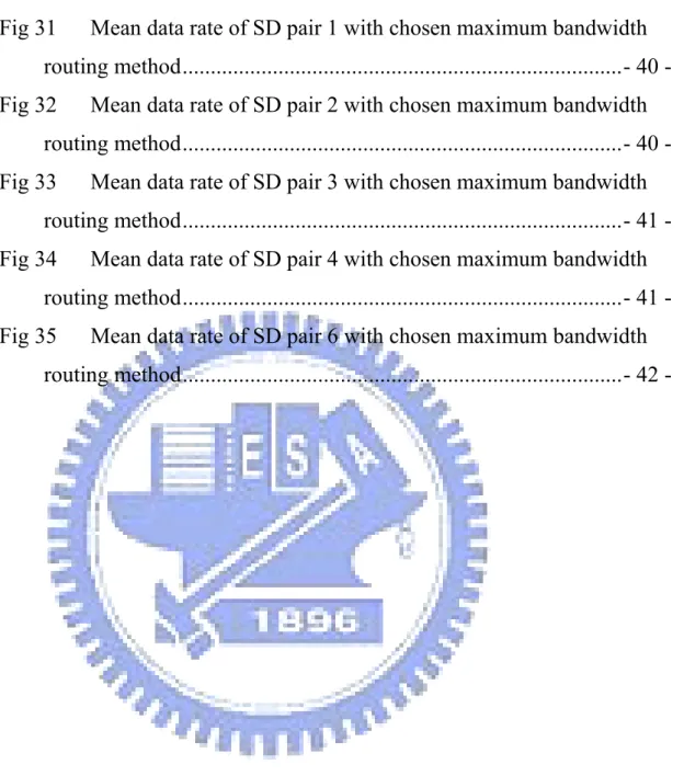
(14) .. congestion links encountered by calls of type i taking path j. x i , j is the sample rate of type i taking path j. Where fi is function of xi, the format of fi(xi) is show as following :. ⋅. ni. f i ( xi ) = log(∑ xi , j ) j =1. (2.2). The parameter xi is rate of each type i and log(．) denotes the natural logarithm, parameter ni means that how many path for type i can choose.. 2.2. Interaction of adaptive control algorithm for dispersity routing In the section, we introduce that how the adaptive control algorithm help routing to. achieve optimal rate allocation for different sources. Basically, the control algorithm will return a sample rate of path belong to different sources. The information of sample rate from different paths will help the control algorithm to decide next step should be increase which one rate of routing path and decrease which one rate of routing path. The control algorithm get the information rely on BECN technique. For the reason, we briefly introduce BECN technique in the following. BECN (back-forward explicit congestion notification) is the class of explicit congestion notification (ECN). As we know, ECN method can use to detect each congestion situation of nodes on every routing path. Like ECN method, BECN technique will detect the congestion on nodes of different routing paths. When BECN detect a node having congestion, it will return a binary signal (For example: parameter bi,j in the control algorithm) to inform the source there occurs congestion on some nodes of routing path. The feedback information of congestion will back forward along the path that the forwarding packets choose. For more explicit explain, we illustrate BECN mechanism in the following figure:. 5.

(15) Fig 1 An example of BECN mechanism As this figure shows, source (S) node sent packet in a given flow to destination (D) node. In the case, source node has two path can reach the destination node. The path 1 includes node 1, 2, 5, and the path 2 includes node 1,3,2,4. Let us assume if node 2 and node 4 occurs congestion or buffer of link is full in these two nodes. Then BECN will feedback two binary signals from node 2 and node 4 to source. One signal will return the message along path 1 and another will return message along path 2. The adaptive control algorithm use iteration method to achieve optimal resource allocation for each sources and rate of multiple paths allocation. The iteration process of continuous-time format show in the below figure:. 6.

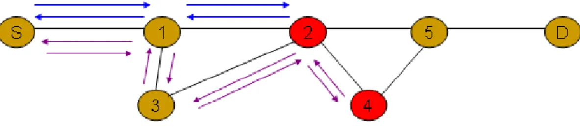
(16) Fig 2. Iteration of adaptive control algorithm. In the figure, the control algorithm is separated as two parts, one part makes decision in the link and another part makes decision in the source. The upper block tells us the information about what is the next strategy of adjusting rate of source that we should do. The lower block bases on the information from the upper block to change the rate of each source. In order to implement this control law in real simulation model, we transfer this continuous-time format to discrete-time format. .. Let. x i , j = g i , j ( x, t ). , then the discrete approximation that we propose is. xid, j [(k + 1)t d ] = x d [ktd ] + t d g i , j ( x(ktd ), ktd );. k = 0,1,.... ,. (2.3). where td is sampling period of each links. As mention in above format, for discrete-time equation, we form our best effort flow control law as following:. 7.

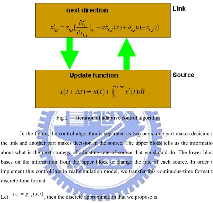
(17) 1. .. x i , j = z i , j (t , x )[. 0.5 + ∑ ji=1 x i , j n. − αbi , j ( x ) − δ i , j u (− xi , j )]. i = 1,2,... j = 1,..., ni (2.4). The function, fi(xi) in our model is formed as following :. ⋅. ni. f i ( xi ) = log(0.5 + ∑ xi , j ) j =1. (2.5). The constant term 0.5 in the logarithm is included to avoid an infinite cost at startup and an infinite derivative of the data rates.. 2.3. Simulation result of TCP flow using adaptive control algorithm for. dispersity routing The adaptive control algorithm is a congestion control method to help us measuring the metric of routing decision and it also approaches optimal rate allocation of different sources by disperity routing. However, the performance of throughput is bad when we apply TCP in the network because if we route packets of a TCP flow to different paths that the RTT of different paths for the TCP flow may have large variance and we may choose a path with low available bandwidth for the TCP flow. The bad simulation result of dispersity routing show in following figure:. 8.

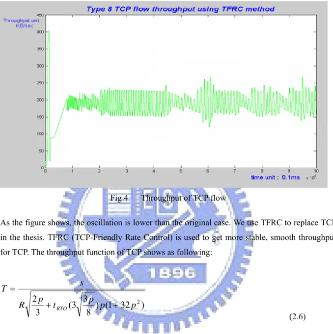
(18) Fig 3. Throughput of TCP flow (without identification flow in router). In the figure, we see that the oscillation of throughput of TCP flow is acutely and we modify the problem by identifying each flow on edge router in the network. One of modified results shows in the following figure:. 9.

(19) Fig 4. Throughput of TCP flow. As the figure shows, the oscillation is lower than the original case. We use TFRC to replace TCP in the thesis. TFRC (TCP-Friendly Rate Control) is used to get more stable, smooth throughput for TCP. The throughput function of TCP shows as following:. s. T= R. 2p 3p + t RTO (3 ) p (1 + 32 p 2 ) 3 8. (2.6). In the throughput function, where s is packet size and R is round-trip time, p is steady state loss event rate, t RTO is TCP retransmit timeout value. TFRC calculate loss event rate take average loss interval method. It can help TCP flows having smoother throughputs in steady state. The following extra sub-section will introduce the average loss interval method and how TFRC define the lost interval.. 10.

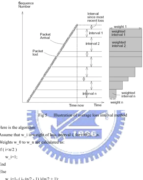
(20) * 2.4. Determine a new lost event interval calculation and Average loss. interval method Average loss interval method take a more smoothly calculation lost event rate than original TCP congestion detection method, that is, congestion window method. Original congestion window control will case AIMD (additive increase/multiplicative decrease). The key of smooth throughput of TFRC is that the new loss probability calculation method defines a lost event not by detecting a lost packet but calculating how many packets in the lost interval to uniformly compute TCP loss probability. TCP defines a lost packet that is the receiver receives a sequence number of packet out of three orders than the sequence number of old packet in TCP receiver end. When a packet loses, we will calculate a false arrival time for the lost packet to determine if we need to update a new loss interval. The algorithm shows in the following: We assume some parameters in the follows before us calculation of the false arrival time: S_loss is the sequence number of a lost packet. S_before is the sequence number of the last packet to arrive with sequence number before S_loss. S_after is the sequence number of the first packet to arrive with sequence number before S_loss. T_before is the reception time of S_before. T_after is the reception time of S_after. T_loss is the false reception time of S_loss. Then the calculation function of T_loss is:. T _ loss = T _ before + (T _ after − T _ before)(. S _ loss − S _ before ) S _ after − S _ before. (2.7). If T_loss+R>T_after, we will need update our old loss event interval to next new lost event interval, the new arrival packet will be calculated into the number of new interval. When we need update our old lost event interval, we also update our loss event probability in the same time. In the other words, we are not so frequently changing loss probability of TCP. We use the following figure to illustration the average lost event interval method. 11.

(21) Fig 5. Illustration of average loss interval method. Here is the algorithm: Assume that w_i is weight of loss interval i, for i=0,2,…,n. Weights w_0 to w_n are calculated as: If ( i<n/2 ) w_i=1; End Else w_i=1- ( i- (n/2 - 1) )/(n/2 + 1); End After determining weights of all intervals, we calculate the average loss interval as follows:. ∑ sˆ = ∑ n. i =1 n. wi si. i =1. wi. ,. (2.8) 12.

(22) for weights wi: wi = 1,. 1≤ i ≤ n/2. and. ∑ w s = ∑ w n −1. sˆnew. i =0 n. i =1. i +1 i i. (2.9). 1 max( sˆ, sˆnew ) The loss event probability then is:. 13. .. (2.10).

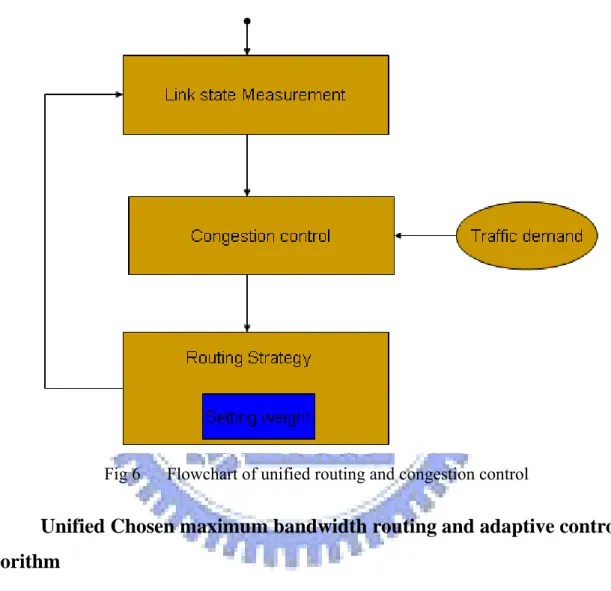
(23) Chapter 3 Unified routing and congestion control. Routing algorithms make routing decisions rely on the feedback information that is proposed by some measurement mechanisms. In the thesis, we had introduced the adaptive control algorithm in chapter 2. Now, in the chapter, we will introduce how to use the adaptive control algorithm to help our routing method making decision. Our routing algorithm is based on the adaptive control algorithm. As mention in chapter 2, the control algorithm will return bandwidth of each path for each source and we use the information as our routing metric. We propose two methods, one is proportion routing and another is choosing maximum bandwidth routing. Our method is very simple and can easily be implemented in really routing management.. 3.1. Introduction of unified routing and congestion control Let us trace the flowchart in the following figure, from start point, we will randomly. route each flow of different sources to different available routing paths. After a period of time, the unified mechanism will measure each buffers size of links to determine if buffer is full or still having free space. If one of buffer in the links is full, then the mechanism will recognize as this link occurs congestion. In the other words, we define congestion as the arrival rate of packets large than the capacity of link. Once the nodes detect congestion they will use BECN mechanism to feedback congestion messages to each source. After measuring link state, the information of congestion will let the congestion control mechanism to deal with and the congestion control needs considering different traffic demands in the control law. In the other words, the block of congestion control will assign different traffic demands to get different control laws. Then the feedback information will be send to their sources and these sources will take some routing strategies to lead flows to the “correct path”. Routing algorithms adjust their decision weights. 14.

(24) when they receive new feedback information. This kind of scenario will continue till to the goal of global achieved is approached. The total flowchart of unified our routing methods and adaptive control algorithm shows in following figure.. Fig 6. 3.2. Flowchart of unified routing and congestion control. Unified Chosen maximum bandwidth routing and adaptive control. algorithm In the following subsection, we will introduce how to use the information xi,j as our routing metrics. As we introduce in section 3.1, when the congestion information is received by the sources, they will add the bi,j value of adaptive congestion control laws and the adaptive congestion control mechanism will re-assign bandwidth for each routing path. According to the information of available bandwidth of each path, we propose the chosen maximum bandwidth method to solve the problem that introduce in chapter 1 .The chosen maximum bandwidth method will choose the path which has maximum bandwidth in all routing paths which belong to. 15.

(25) a source. This kind of routing decision likes as gradient decent method of optimal theory. We will approach the optimal point by leading each new arrival flow away from the most congestion path. The form of routing decision of “chosen maximum bandwidth” method is:. i∈Ω. Max( xi , j ), j∈ni. Where parameter. ,where Ω is all sources in the network.. xi , j. (3.1). is sending rate (available bandwidth of paths) of source i taking path j and. parameter ni means how many path source i can choose to route flows. Let us more explicit introduce the method by the following example: Consider in the network having two sources, source 1 owns four paths to route the flow to destination and source 2 owns three paths to route the flow to destination. We get the information of available bandwidth for each path belongs to the source periodically. Let us define the four paths which belong to source 1 as p11, p12, p13, p14 and the three paths which belong to source 2 as p21, p22, p23. For their individual available bandwidth, we express them as x11, x12, x13, x14 and x21, x22, x23. When we use chosen maximum bandwidth method to choose the suitable routing path for the new arrival flow, we compare the value like this: For source 1:. For source 2:. if (x11>x12>x13>x14). if (x21>x22>x23). take path p11;. take path p21;. end. end. else if (x12>x11>x13>x14). else if (x22>x21>x23). take path p12;. take path p22;. end. end. else if (x13>x11>x12>x14). else if (x23>x21>x22). take path p13;. take path p23;. end. end. else if (x14>x11>x12>x13). else. take path p14;. take shortest path;. 16.

(26) end. end. else take shortest path; end. 3.3. Unified proportion routing and adaptive control algorithm In the section we will introduce another method, which is, using the available bandwidth. of each routing path as weights to randomly route the new arrival flows to a path. The kind of routing method generally calls as proportion routing method. Proportion routing is commonly applying in routing area and it can efficiently distribute flows in different routing path based on the weight proportion of routing metric. Our method uses the feedback bandwidth of each path by adaptive control algorithm. When a new arrival flow comes, we can assign the flow to a path by a probability which generates by the rate of the available bandwidth of each routing path. The form of routing decision of proportion routing shows in the following:. xi , j. ∑. ni j =1. xi , j. .. Where parameter parameter. (3.2). xi , j. is sending rate (available bandwidth of paths) of source i taking path j and. ni means how many path source i can choose to route flows.. Let us more explicit introduce the method by using the example in section 3.2: In the above case, we know that there are two sources in the network and source 1 has four available routing paths, source 2 has two available routing paths. Once again, we use the information of available bandwidth for each path which provides by adaptive control algorithm as our routing metric. When a new arrival flow comes, we take the following strategy: We first generate a random number a and the value of a is between 0 to 1 ( 0 < a ≤ 1 ).. 17.

(27) For Source 1: if (0 < a <=. x11 ) x11 + x12 + x13 + x14. take path p11; end else if (. x11 x12 < a <= ) x11 + x12 + x13 + x14 x11 + x12 + x13 + x14. take path p12; end else if (. x13 x12 < a <= ) x11 + x12 + x13 + x14 x11 + x12 + x13 + x14. take path p13; end else take path p14; end For source 2: if (0 < a <=. x 21 ) x 21 + x 22. take path p21; end else take path p22; end. 18.

(28) Chapter 4 Simulation. In the following figure, we take the figure of network as our simulation topology. In the figure, we have eight sources and the transmission delays of each links, the capacity of each links are show in the figure. Our assumption is all sources can generate TCP traffic randomly. All TCP traffics implement by TFRC and queue management for buffer of link is FIFO. We also assume some paths of eight source-destination pairs in the following table.. Fig 7. Topology of network. 19.

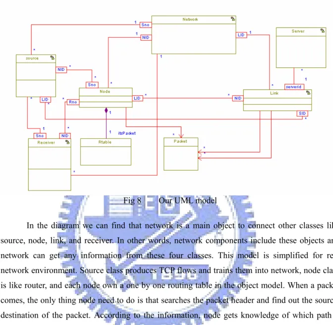
(29) These sources could route paths we form as a routing path table, show as following: Table 1. All available paths for all SD pairs. The notation ni i=1,2,3,4,5,6,7,8 means how many paths each type can route in the network topology.. 4.1. Simulation model introduction We assume all TCP flows randomly appear and each flow has different lifetime and we. take the first in first out (FIFO) queue management in our simulation. Meanwhile, when the queue of link is full, we take tail drop strategy. Our simulation take UML to help build model. We build a network environment show in the following object main diagram:. 20.

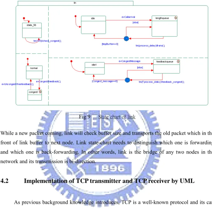
(30) Fig 8. Our UML model. In the diagram we can find that network is a main object to connect other classes like source, node, link, and receiver. In other words, network components include these objects and network can get any information from these four classes. This model is simplified for real network environment. Source class produces TCP flows and trains them into network, node class is like router, and each node own a one by one routing table in the object model. When a packet comes, the only thing node need to do is that searches the packet header and find out the source, destination of the packet. According to the information, node gets knowledge of which path it should transport these passing through packets. When node transports these packets into next node, the state-chart of link get starting and will check that buffer size is full or still has space. The state-chart of link shows in the following figure.. 21.

(31) Fig 9. State chart of link. While a new packet coming, link will check buffer size and transports the old packet which in the front of link buffer to next node. Link state-chart needs to distinguish which one is forwarding and which one is back-forwarding. In other words, link is the bridge of any two nodes in the network and its transmission is bi-direction.. 4.2. Implementation of TCP transmitter and TCP receiver by UML As previous background knowledge introduces, TCP is a well-known protocol and its can. be replaced by TCP friendly protocol. Also we know that stability of TCP based on end to end congestion control mechanism. The following we will implement our TFRC flow model by UML and illustrate how they work together. The state-chart of TCP transmitter show in the following figure:. 22.

(32) Fig 10. State chart of TCP transmitter. In the figure, we can see that TCP transmitter will send packets of flows into ingress node of network and receive ack message in the same time. TCP transmitter also needs to record RTT value in order to determine the next packet sending time. As the state-chart shows, in “intime” state, if “end_time>nofeedback_time” means TCP under slow-start state and need double original TCP data rate else means TCP under stable state and data rate not need change (see [10] p.10). TCP lifetime also determine by transmitter. Transmitter will continue sent packet until the parameter “TCPlifetime” lower than 0. When receiver receives a packet, it must distinguish packet number if out of order (the sequence number of new arrival packet is out of 3 sequence number than the number of old packet) and if update the loss-event interval need introduce in background knowledge section. The state-chart of receiver illustrates in the following figure. In the figure, we can see that receiver only need to do one thing. That is, we mention before the “out of order packet check”. The design of main ideal of TFRC mechanism is that the receiver should be as possible as simply and let transmitter to deal with most works.. 23.

(33) Fig 11. 4.3. State chart of TCP receiver. Compare for SPR and our routing method Our simulation compares three methods results, the first is shortest path routing method. (SPR), and the second is proportion routing method, finally, we show choose maximum bandwidth routing method result. For all eight sources simulation, we only discuss the results of source 5,7,8 because the results of source 5,7,8 have unique meaning on choosing paths for total network topology. The following figures show the mean data rate of source 5,7,8 using shortest path routing method. From my simulation, I observe that the original shortest path method makes TCP flow of source 7 having un-uniformly throughput show in the following figures. This means that some flows in source 7 may get bad throughputs because source 7 needs to share bandwidth with source 3,4. For source 5 and source 8, they are show the uniform distribution of throughput in Fig 12 and Fig 14 because no other sources will share their bandwidth on their paths.. 24.

(34) Fig 12. Mean data rate of SD pair 5 with SPR method. Fig 13. Mean data rate of SD pair 7 with SPR method. 25.

(35) Fig 14. Mean data rate of SD pair 8 with SPR method. Because the bad result of source 7, we try to use proportion routing method and choose maximum bandwidth method to improve all user’s throughput fairness and let network manger approach maximum utilize buffer of link. These results show as following figures:. 26.

(36) Fig 15. Mean data rate of SD pair 5 with proportion routing method. Fig 16. mean data rate of SD pair 7 with proportion routing method. 27.

(37) Fig 17. Fig 18. mean data rate of SD pair 8 with proportion routing method. Mean data rate of SD pair 5 with chosen maximum bandwidth method. 28.

(38) Fig 19. Mean data rate of SD pair 7 with chosen maximum bandwidth method. Fig 20. Mean data rate of SD pair 8 with chosen maximum bandwidth method. 29.

(39) In the results of choose maximum bandwidth routing method, it gets more uniform distribution for throughput of each flows of individual source-destination pairs. Individual source-destination pairs get well utilization in each links because we unite routing and adaptive control algorithm. It looks like that the fairness of choosing maximum bandwidth routing method is better than proportion routing and shortest path routing. However, the global fairness of chosen maximum bandwidth routing is not the best. In order to show the global fairness is really not the best, we compare again the fairness for all source-destination pairs by our global fairness index. The function of global fairness index is:. (∑∑ xij ) 2 i. j. n∑∑ xij2 i. j. (4.1). The table 1 lists results of three methods: Table 2. Global fairness index of three methods. In the table 2, we can see that the global fairness of proportion routing method is best and chosen maximum bandwidth routing is less about 0.02 percent for global fairness index, shortest path routing is less about 0.2 percent for global fairness index. Form the above results of simulation; we guess that when the fairness index increases then the throughput of each flow will decrease. In order to prove the phenomenon is rally truly, we also measure the mean throughput for three methods in the table 3.. 30.

(40) Table 3. Average throughput of three methods. In table 3, we can see that the mean throughput of SPR is highest, throughput of chosen maximum bandwidth routing lessees about 600 packets per flow than SPR and the worse case is proportion routing, it lessees about 1100 packets per flow than SPR. It shows that if we want to get good global fairness then our total throughput will decrease at the same time.. 31.

(41) Chapter 5 Conclusion and Future work. In the thesis we propose two routing methods that unify congestion control and they improve the total fairness among different source-destination pairs. The two methods only base on binary feedback information to configure their routing strategies. According to our simulation, the proportion routing method can achieve to 82 percent for global fairness index. However, the mean throughput will be reduced to about 2900 packets per flow. For this kind of result, we guess that using SPR method does not spent the bandwidth of other TCP flows in their original paths and using proportion routing may spend the bandwidth of other TCP flows cause the throughput of flows decreasing. How to solve this problem is the biggest work for us. For the further research, maybe we can trade off between fairness and throughput by adding some parameters to configure them to approach a balancing situation. The parameters can like as flows number in a path etc.. 32.

(42) References [1] Emilio Leonardi, Marco Mellia, Marco Ajmone Marsan, Fabio Neri, “Joint Optimal Scheduling and Routing for Maximum Network Throughput”, IEEE/INFOCOM VOL 2, 2005, pages 819-830. [2] Constantino Lagoa, Hao Che and Bernardo A. Movsichoff, “Adaptive Control Algorithms for Decentralized Optimal Traffic Engineering in the Internet”, IEEE/ACM TRANSACTIONS ON NETWORKING 2004, 12(3):415-428. [3] Anindya Basu, Alvin Lin, Sharad Ramanathan, “Routing Using Potentials: A Dynamic Traffic-Aware Routing Algorithm”, ACM SIGCOMM, August 25-29, 2003. [4] Sally Floyd, Mark Handley, Jitendra Padhye, “Equation-Based Congestion Control for Unicast Applications: the Extended Version*”, March 2000. ICSI Technical Report TR-00-03, URL http://www.aciri.org/tfrc/. [5] R. J. La and V. Anantharam, “Charge-sensitive TCP and rate control in the Internet,” in Proc. IEEE INFOCOM, Mar. 2000, pp. 1166–1175.. [6] F. Bonomi and K. W. Fendick, “The rate-based flow control framework for the available bit rate ATM service,” IEEE Network, vol. 9, no. 2, pp. 25–39, Mar./Apr. 1995. [7] N. F. Maxemchuk, “DISPERSITY ROUTING”, Proceedings. of ICC, June 1975, pp. 41.10-41.13. [8] P. Newman, “Traffic Management for ATM Local Area Networks,” IEEE Communications Magazine, pp.44-50, August. 1994.. 33.

(43) [9] S. Floyd, E. Kohler, “TCP Friendly Rate Control (TFRC): The Small-Packet (SP) Variant”, April 2007.URL http://www.ietf.org/rfc/rfc4828.txt.. 34.

(44) Appendix A. Fig 21. Mean data rate of SD pair 1 with SPR method. Fig 22. Mean data rate of SD pair 2 with SPR method. 35.

(45) Fig 23. Mean data rate of SD pair 3 with SPR method. Fig 24. Mean data rate of SD pair 4 with SPR method. 36.

(46) Fig 25. Fig 26. Mean data rate of SD pair 6 with SPR method. Mean data rate of SD pair 1 with proportion routing method. 37.

(47) Fig 27. Mean data rate of SD pair 2 with proportion routing method. Fig 28. Mean data rate of SD pair 3 with proportion routing method. 38.

(48) Fig 29. Mean data rate of SD pair 4 with proportion routing method. Fig 30. Mean data rate of SD pair 6 with proportion routing method. 39.

(49) Fig 31. Mean data rate of SD pair 1 with chosen maximum bandwidth routing method. Fig 32. Mean data rate of SD pair 2 with chosen maximum bandwidth routing method. 40.

(50) Fig 33. Mean data rate of SD pair 3 with chosen maximum bandwidth routing method. Fig 34. Mean data rate of SD pair 4 with chosen maximum bandwidth routing method. 41.

(51) Fig 35. Mean data rate of SD pair 6 with chosen maximum bandwidth routing method. 42.

(52) Appendix B Table 4. Local fairness index of three methods. 43.

(53)