投資期間、函數型態與共同基金之評估---靜態與動態之分析

(1)

行政院國家科學委員會補助專題研究計畫 - 成果報告

計畫名稱：投資期間、函數型態與共同基金之評估: 靜態與動態之分析

Investment Horizon, Functional Form and Mutual Fund

Evaluation: Static vs. Dynamic Approach

計畫類別：V 個別型計畫 □

整合型計畫

計畫編號：NSC 92-2416-H-009-018

執行期間：92 年 8 月 1 日至 93 年 7 月 31 日

計畫主持人：

李正福

共同主持人：

林建榮

計畫參與人員：

劉炳麟、魏曉琴、黃曉芸、柯玫伶、陳衍龍、莊亨懋、

陳孟雅、施冠宇、李嘉炎、謝碧鳳、袁惠芸、王順瓔、蘇文淇、彭宜屏

成果報告類型(依經費核定清單規定繳交)：V 精簡報告 □完整報告

本成果報告包括以下應繳交之附件：

□赴國外出差或研習心得報告一份

□赴大陸地區出差或研習心得報告一份

□出席國際學術會議心得報告及發表之論文各一份

□國際合作研究計畫國外研究報告書一份

處理方式：除產學合作研究計畫、提升產業技術及人才培育研究計畫、

列管計畫及下列情形者外，得立即公開查詢

□ 涉及專利或其他智慧財產權，□一年□二年後可公開查詢

執行單位：國立交通大學財務金融所

(2)

2

I. 中英文摘要及關鍵詞(keywords)

（一）計畫中文摘要 計畫名稱：投資期間、函數型態與共同基金之評估: 靜態與動態之分析 關鍵詞：投資期間、函數型態、共同基金、基金評估、靜態分析、動態分析 不論對個人或法人投資者而言，共同基金都是最重要的投資方式之一；因此，共同基金績效的評估始終是財務學上最重要的研究標的之一。此研究計畫的目的在將本人以往研究之成果加以整合並普及化(見參考資料)。第一階段先發展一個總括性的函數型態模型來評估共同基金的績效。第二階段再以這個總括性的函數型態模型進行調查各種投資期間組合對基金績效表現的影響，利用2883 種基金的每個月資料來研究各個投資期間的基金表現。最後，利用跨期 CAPM 模型對上述之資料進行共同基金績效之評估。換言之，此研究以靜態及動態兩種方式來評估共同基金之績效表現。（二）計畫英文摘要

Title: Investment Horizon, Functional Form and Mutual Fund Evaluation: Static vs. Dynamic Approach

Key Words: Investment Horizon, Functional Form, Mutual Fund Evaluation, Static Approach, Dynamic Approach

Mutual fund is one of the most important investment products for both individuals and institutional investors. Therefore, mutual fund performance evaluation is one of the most important research topics in finance. The main purpose of this research is to integrate and generalize my previous important research results [see Lee, Cheng F. 1976; Lee, Cheng F. 1977; Fubozzi, Frank J. (1980); Lee, Cheng F., Chunchi Wu, and K.C. John Wei, 1990; Lee, Cheng F. and Shafiqur Rahman 1990; Lee, Cheng F. and Shafiqur Rahman, 1994, and Chang Jow-ran, Mao-wei Hung and Cheng F. Lee 2002].

In this research, firstly I develop a generalized functional form model for mutual performance evaluation. Secondly, this generalized functional form is used to investigate the impact of investment horizon on the performance of mutual funds. To do this, monthly data of 2883 mutual funds are used to study the investment horizon on mutual fund performance. Finally, generalized αand β are calculated to study dynamic nature of mutual fund performance measures. In sum, this study uses both static and dynamic models to evaluate mutual performance.

(3)

I. 報告內容

The main results of this project include two parts as follows:

Part One: Generalized Functional Form for Alternative Mutual Fund Returns

Abstract

Based upon the paper by Fabozzi, Francis and Lee [1980, JQFA], we investigate the generalized functional form relationship for 23 alternative mutual funds in terms of the monthly data during 1992 to 2002. Implications of the functional form for mutual fund performance are analyzed in detailed. New performance measures are also explored. Further research suggestions are also discussed.

A. Introduction

Based on the theory of the pricing of capital assets developed by Sharpe [1964], Lintner [1965] and Mossin [1966], Professor Jensen Formulated a return-generating model to measure

portfolio performance [1968] in a subsequent paper, Professor Jensen [1969] investigated the impact of the investment horizon on the functional form of the model. Lee [1976] has proposed a generalized specification of the model to resolve this problem. Alternative estimation

methods for testing the linearity of the model in terms of time-series data have also been

suggested by Lee. Moreover, the stability of the beta coefficient over time and the impact of the market’s condition on both the alpha (or Jensen’s measure of Performance [1968]) and beta of the model have come under scrutiny in financial research.(1) Fabozzi, Francis and Lee has used generalized functional form approach to investigate the mutual performance measure for 10 large growth funds, 22 smaller growth funds, 11 income funds, 13 balanced funds and 30 diversified common stock funds.

The main purpose of this paper is to update and extend the scope of mutual fund in terms of Fabozzi, Fancis and Lee’s model. Some new empirical implications are investigated in detailed. The paper is organized as followed; the second section of the paper defines the generalized return-generating model. The third section describes the data in detailed; the fourth section presents the empirical results. Finally, in section five, results of the paper are summarized and some concluding results are discussed.

(4)

4 B. The Generalized Rate of Return-Generating Model

Following Lee [1976], the generalized model used to investigate the mutual fund rates of return-generating process without error term can be defined as:

Rjt* − Rft* = αj + βj [Rmt* − Rft*] (1) where:

Rjt* = (Rjtλ − 1) / λ, Rft* = (Rftλ − 1) / λ, Rmt* = (Rmtλ − 1) / λ,

λ = the functional form parameter,

Rjt = 1 + the rate of return for the jth mutual fund in period t, Rmt = 1 + the market rate of return in period t,

Rft = 1 + the risk-free rate of interest in period t, βj = the systematic risk for the jth mutual fund, and αj = the intercept term for the jth mutual fund. Equation (1) can be rewritten as:

Rjt* = αj + (1 − βj) Rft* + βj Rmt*. (2)

Equation (2) is a constrained or restricted regression. The relationship is similar to that of Zarembka [14, pp. 502-504]. Equation (1) reduces to the linear function form if λ is equal to unity.1 If the function form parameter λ approaches zero, then equation (1) reduce to

(log Rjt − log Rft) = αj + βj (log Rmt − log Rft). (3)

The estimated βj is Jensen’s instantaneous systematic risk and the estimated αj is the Jensen’s performance measure in equation (3).

(5)

III. Impact of the Functional Form on the Parameters of the Model: Some Analytical Results

Based upon Taylor’s expansion, we have

... ) (log ! 3 1 ) (log ! 2 log 1 2 3 log ₌ ₊ ₊ ₊ ₊ z z z e z λ

Equation (1) implies that

) 4 ( ... ) (log ! 3 ) (log ! 2 log ] 1 ... ) log ( ! 2 1 log 1 [ 1 1 3 2 2 2 + + + = − + + + = − t t t t t t Y Y Y Y Y Y

λ

λ where Y_t =R_jt_'R_mt or R_ft

Equation (3) implies that (Y_tλ −1) /λ can be approximated by logY if the higher order terms _t are trivial. The conditions for the higher order terms to be trivial are: 1) λ approaches zero; and 2) the higher order terms of logY are small. The latter condition depends upon the _t

observation period. If monthly returns are used, then the higher order terms of logY are _t generally small. Therefore, the ˆα_j and ˆβ_j estimated from logY will not be significantly _t different from those estimated from (Y_tλ −1) /λ.

Following Zarembka [14, p.503], the intercept of equation (1) can be defined as

* * 1 . (5) j j for some λ α _α λ −

If either λ approaches zero or * j

α

is small, then, following equation (4) , we can argue that (5) is approximately equal to _log *

j

α

, where _log * j

α

is the Jensen performance measure for the logarithmic-linear model.

Jensen [5, p.394] investigated the impact of the intertemporal instability of beta on the model. Here we shall consider the implication of the functional form on the beta coefficient in terms of an elasticity framework.

(6)

6

If λ approaches zero, then the estimated beta is the elasticity between (logRjt −logRf t) and (logRmt −logRf t). If λ is significantly different from zero, then the elasticity is a function of R , mt R and jt λ. Since Rmt /R may vary over time, jt

η

t may not be intertemporally

stable. If the ratio between the market return, R , and return for the mt th

j fund, R , which _jt will be denoted by k, is used to used to estimate the elasticity

η

_t, then we can analyze the bias associated with

η

_t as follows:

(A) λ is positive

(i) if k > 1, then the elasticity obtained from equation (3)underestimates the

η

_t.

(ii) if k < 1, then the elasticity obtained from equation (3) overestimates the

η

_t. (B) λ is negative

(i) if k > 1, then the elasticity obtained from equation (3) overestimates the

η

_t.

(ii) if k > 1, then the elasticity obtained from equation (3) underestimates the

η

_t.

C. Description of Data

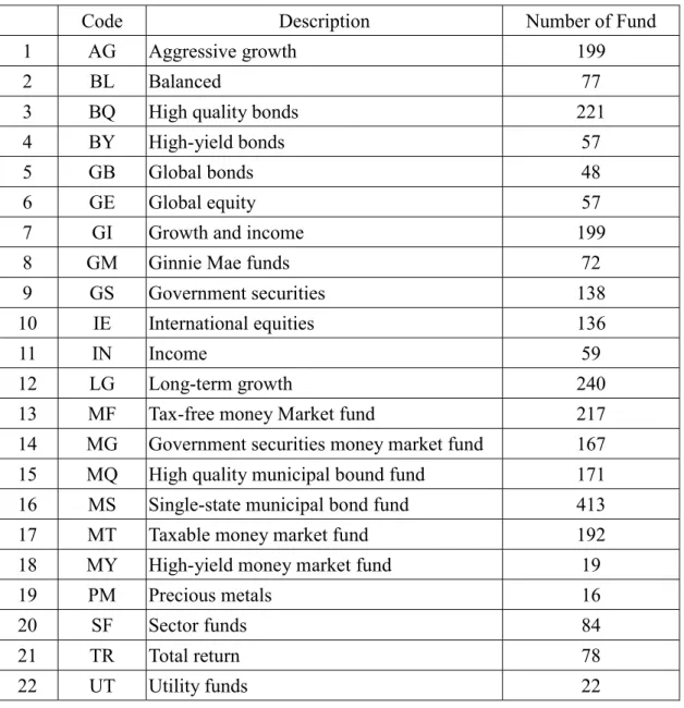
Monthly data of 22 mutual funds during January 1993- June 6, 2002 are collected from CRSP Tape to do the generalized functional form analysis. This 22 mutual fund are 1. Aggressive growth 2. Balanced, 3. High quality bonds, 4. High-yield bonds, 5. Global bonds, 6. Global equity, 7. Growth and income, 8. Ginnie Mae funds, 9. Government securities, 10. International equities, 11. Income, 12. Long-term growth, 13. Tax-free money market fund, 14. Government securities money market fund, 15. High quality municipal bound fund, 16. Single-state

municipal fond fund, 17. Taxable money market fund, 18. High-yield money market fund, 19. Precious metals. 20. Sector funds, 21. Total return, 22. Utility funds. Other detailed information for these 22 mutual fund are described in Table 1.

D. Empirical Result

First, Based upon equation (1), we estimate the functional form parameter,λ, then we based upon equation (3), we estimate the beta , the estimated lambda and beta and other related information for different mutual funds. Summary measures for all the 22 different kinds of mutual funds are presented in Table A-1 through Table A-22 in Appendix A. Last column of each table J-B represents Jarque-Bera statistic which are used to test the normal distribution of each estimate.

(7)

To determine the functional form parameter, Rjt, Rmt and Rft were transformed in accordance

with equation (1) using λ’s between -5 and 5 at intervals of .12. Hence, 101 different regressions were estimated for each fund. For each regression, the logarithmic maximum likelihood value, given by equation (7), was computed. The functional form value that corresponds to the highest value for L max (λ) is then the optimal value,λ∧ .

) 7 ( tan log ) 1 ( ) ( log ) max( 1 t cons R n L n t jt e + − + − =

∑

= λ λ σ λ

where n is the sample size and σe(λ) is the estimated regression residual standard error of

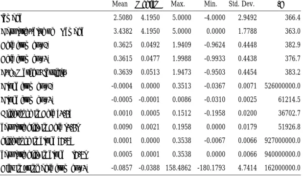
equation (2). Summary measures for the optimal λ∧ are shown in rows one of Tables A1 - A22 in Appendix A, while the distribution of λ∧ is summarized in the first column of Table 3. The mean and median optimal λ∧ for the 2883 funds were 2.5084 and 4.1950, respectively.

Using the likelihood ratio, an approximate 95 percent confidence region for the optimalλ∧ for each fund can be obtained from equation (8).

) 8 ( 92 . 1 ) 05 (. 2 / 1 ) max( ) ˆ max( 2 1 = < −L X L λ λ

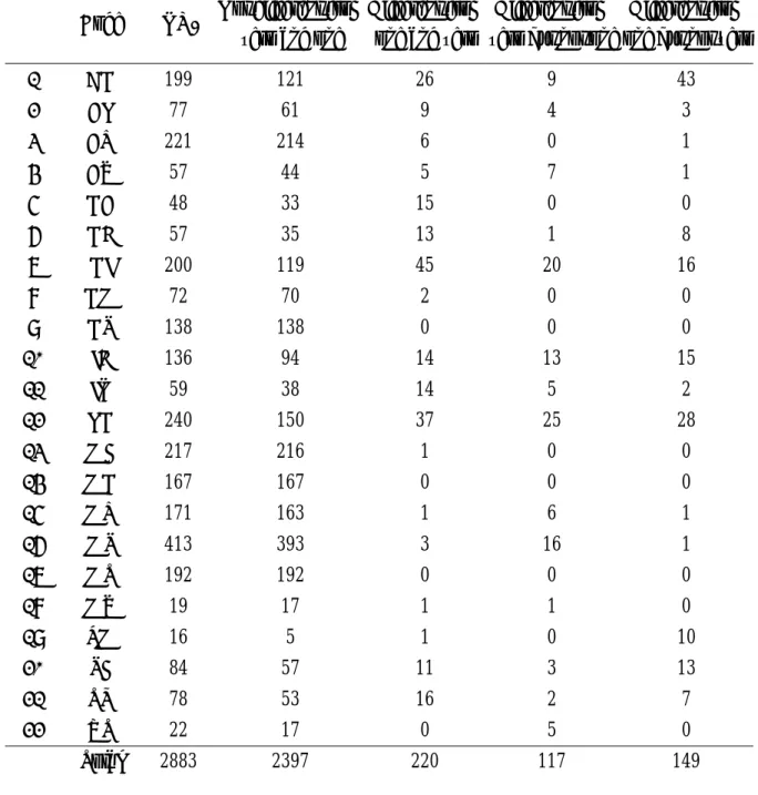
A 95 percent confidence interval was computed for each mutual fund and these intervals were used to determine whether the functional relationship is significantly different from one and/or zero. The results are summarized in columns 2 through 5 in Table 3. 220 funds exhibited a functional relationship the different significantly from both the linear and logarithmic linear form. For 117 funds the hypothesis that the functional form was logarithmic-linear was rejected. The linear form was rejected for 140 funds.

The market elasticity was calculated in accordance with equation (6). This equation shows that the market elasticity can be decomposed into the following two components: (i) the beta coefficient estimated using equation (2); and, (ii) an adjustment factor for period i given by (

jt mt

R R

)λ. The third row of Table 1 presents summary measures for the estimated beta coefficient using equation (2). The fifth row presents the average market elasticity which was computed for an individual fund as follows:

(8)

8 114 / ) ˆ ( 114 / ) ( 114 1 ˆ 114 1

∑

= = = = t t j t t k n β λ η

To test whether the estimate lambda is significantly different from 1 and 0, we present the distribution table of estimated lambda for each mutual fund. For example, in Table 3, column 4, there are 2397 estimated lambda. They are not different from 1 and 0. In column 5, indicates that there are 220 estimated lambda, which are different from 1 and 0. In column 6, indicates that there are 117 estimated lambda, which are different from 0 but not 1. In column 7, indicates that there are 149 estimated lambda, which are different from 1 but not 0.

1 ) / ˆ (βj η − ] 114 / ) / ( [ 114 1

∑

= = t jt mt R R K ) 9 ( ) log (log ) log (log ) log (log 2 ft mt j ft mt j j ft jt R R R R R R − + − + = −

γ

β

α

λ λ λ₍₁

_β

₎

_β

_]1/ [ ft j mt j jt R R R = − + terms order higher R R R R R_j _j _mt _ft _j _mt _ft + − + −

= _(log _log ₎ _(log _log ₎2

log

β

γ

where (1 ) 2 1 j j j

λβ

β

γ

= −

E. Summary Conclusion and Remark

Based upon generalized investment horizon type of CAPM which was derived by Lee

[1976,1977], Fubozzi [1980], Lee et al. [1990], we used monthly data of 2884 mutual funds to estimate generalized αand β. In addition, we also found that there are significantly in

estimated λ’s among 22 types of mutual funds. In conclusion, the generalized functional form is important in evaluate the performance of different type of mutual fund.

References:

Admati, A.R., S. Bhattacharya and P. Pfleiderer. 1986. “On Timing and Selectivity” Journal of Finance. 41. 715-730

Baks, Klaas P., Andrew Metrick and Jessica Wachter. 2001. "Should Investors Avoid All Actively Managed Mutual Funds? A Study in Bayesian Performance Evaluation" Journal of Finance, 56(1), 45-85

(9)

Becker,Connie, Wayne Ferson, David H.Myers and Michael J.Schill. 1999. "Conditional Market Timing with Benchmark Investors" Journal of Financial Economics, 52, 119-148 Blume, M. and I. Friend. 1973. “A New Look at the Capital Asset Pricing Model” Journal of

Finance, 28, 19-33

Bollen, Nicolas P.B., and Jeffrey A. Busse. 2001. "On the Timing Ability of Mutual Fund Managers" Journal of Finance, 56(3), 1075-1094

Brown, Stephen J. and William N. Goetzmann. 1997. “Mutual Fund Styles” Journal of Financial Economics, 43, 373-99

Brown, Stephen J. and William N. Goetzmann. 1995a. “Attrition and Mutual Fund Performance” Journal of Finance, 50, 679-698

Brown, Stephen J. and William N. Goetzmann. 1995b. “Performance Persistence” Journal of Finance, 50, 679-698

Brown, Stephen J. and William N. Goetzmann, and Stephen A. Ross. 1992. “Survivorship Bias in Performance Studies” Review of Financial Studies, V5 (4), 553-380

Brown, Stephen J. and William N. Goetzmann, and Stephen A. Ross. 1995. “Survival” Journal of Finance, 50,853-873

Brown, Stephen J. and William N. Goetzmann, Takato Hiraki, Toshiyuki Otsuki and Noriyoshi Shiraishi. 2001. "The Japanese Open-End Fund Puzzle" Journal of Business, 74(1), 59-77 Busse, A. Jeffrey. 1999. "Volatility Timing in Mutual Funds: Evidence from Daily Returns"

The Review of Financial Studies, 12(5), 1009-1041

Calson, R. 1977. "Aggregate Performance of Mutual Fund, 1948-1967" Journal of Financial and Quantitative Analysis, 5, 1-32

Carhart, Mark M. 1997. "On Persistence in Mutual Fund Performance" Journal of Finance, 52(1), 57-82

Carpenter, N. Jennifer, and Anthony W. Lynch. 1999. "Survivorship Bias and Attrition Effects in Measures of Performance Persistence" Journal of Financial Economics, 54, 337-374 Chang, Eric C. and Wilbur G. Lewellen. 1984. "Market Timing and Mutual Fund Investment

Performance" Journal of Business, V57 (1), 57-72

Chang, Jow-Ran, Mao-wei Hung, and Cheng-few Lee. 2002. “An Intertemporal CAPM Approach to Evaluate Mutual Fund Performance”, FMA Annual Meeting, San Antonio, Chaudhury, M.M and Cheng-few Lee. 1997. "Functional Form of Stock Return Model: Some

International Evidence" The Quarterly Review of Economics and Finance, V37 (1), 151-183

Chen, N.F., R.R. Roll and S.A.Ross. 1986. "Economic Forces and the Stock Market" Journal of Business, 59, 383-403

Chen, C.C. and Cheng F. Lee. 1997. "An Empirical Investigation of the Performance Comparisons between Alternative Asset Pricing Model" Advances in Quantitative Analysis of Finance and Accounting, V5, 117-135

Connor,G. and R. Korajczyk. 1991. "The Attributes, Behavior and Performance of U.S. Mutual Funds" Review of Quantitative Finance and Accounting. V1, 5-26

(10)

10

1035-1058

Edelen, M. Roger. 1999. "Investor Flows and The Assessed Performance of Open-end Mutual Funds" Journal of Financial Economics, 53, 439-466

Elton, Edwin J., and Martin J.Gruber, and Christopher R.Blake. 1995. "Fundamental Economic Variables, Expected Returns and Bond Fund Performance" Journal of Finance. 50, 1229-1256

Elton, Edwin J., and Martin J.Gruber, and Christopher R.Blake. 1996a. "Survivorship Bias and Mutual Fund Performance" Review of Financial Studies, 9, 1097-1120

Elton, Edwin J., and Martin J.Gruber, and Christopher R.Blake. 1996b. "The Persistence of Risk-adjusted Mutual Fund Performance" Journal of Business, 69(2), 133-157

Fabozzi, Frank J., Jack C. Francis and Cheng F.Lee. 1980. "Generalized Functional Form for Mutual Fund Returns" Journal of Financial and Quantitative Analysis, V15 (5), 1107-1120

Fama, Eugene. 1970. "Efficient Capital Markets: A Review of Theory and Empirical Work" Journal of Finance. V25, 383-417

Fama, Eugene. 1991. "Efficient Capital Markets: II" Journal of Finance, 46, 1575-1617

Fama, E.F. and K.R.French. 1992. "The Cross-section of Expected Stock Returns" Journal of Finance, 47, 427-465

Ferson, Wayne E. and Rudi W. Schadt. 1996. "Measuring Fund Strategy and Performance in Changing Economic Conditions" Journal of Finance, 51, 425-461

Goetzmann, N. William, Jonathan Ingersoll Jr., and Zoran Ivkovic. 2000. "Monthly Measurement of Daily Timers" Journal of Financial and Quantitative Analysis, 35(3), 257-290

Grinblatt, Mark and Sheridan Titman. 1989. "Mutual Fund Performance: An Analysis of Quarterly Portfolio Holdings" Journal of Business, 62, 394-415

Grinblatt, Mark and Sheridan Titman. 1992. "The Persistence of Mutual Fund Performance" Journal of Finance, 47, 1977-1984

Grinblatt, Mark and Sheridan Titman. 1993. "Performance Measurement without Benchmarks: An Examination of Mutual Fund Returns" Journal of Business, 66, 47-68

Grinblatt, Mark and Sheridan Titman. 1994. "A Study of Mutual Fund Returns and Performance Evaluation Techniques" Journal of Financial and Quantitative Analysis, 29, 419-444

Grossman, S. and J.Stiglitz. 1980. "On the Impossibility of Informationally Efficient Markets" American Economic Review, 70, 393-408

Gruber, Martin J. 1996. "Another Puzzle: The Growth in Actively Managed Mutual Funds" Journal of Finance, 51, 783-810

Hendricks, Darryll, Jayendu Patel and Richard Zeckhauser. 1993. "Hot Hands in Mutual Funds: Short-run Persistence of Relative Performance, 1974-1988" Journal of Finance, 48, 93-130

Henrikkson, Roy D. and Robert C. Merton. 1981. "On Market Timing and Investment Performance. П. Statistical Procedure for Evaluating Forecasting Skills" Journal of Business, v54 (4), 513-534

Ippolito, Richard A. 1989. "Efficiency with Costly Information: A Study of Mutual Fund Performance 1965-1984" Quarterly Journal of Economics, 104, 1-23

(11)

Jagannathan, Ravi and Robert A. Korajczyk. 1986. "Assessing the Market Timing Performance of Managed Portfolios" Journal of Business, v59 (2), 217-236

Jensen, M.C. 1968. "The Performance of Mutual Funds in the Period 1945-1964" Journal of Finance, 23, 389-416

Kon, S. and Jen. 1979. "Investment Performance of Mutual Funds: An Empirical Investigation of Timing, Selectivity and Market Efficiency" Journal of Business, 52, 263-289

Kothari,S.P., and Jerold B. Warner. 2001. "Evaluating Mutual Fund Performance" Journal of Finance, 56(5), 1985-2010

Kryzanowski, Lawrence, Simon Lalancette and Minh Chau To. 1997. "Performance Attribution Using an APT with Prespecified Macrofactors and Time-Varying Risk Premia and Betas" Journal of Financial and Quantitative Analysis, 32(2), 205-224

Lebmann, B. and D. Modest. 1987. "Mutual Fund Performance Evaluation: A Comparison of Benchmarks and Benchmark Comparisons" Journal of Finance, 42, 233-265

Lee, Cheng F. 1976. "Investment Horizon and the Functional Form of the Capital Asset Pricing Model" Review of Economics and Statistics, 58(3), 356-363

Lee, Cheng F. 1977. "Functional Form, Skewness Effect, and the Risk-Return Relationship" Journal of Financial and Quantitative Analysis, 12(1), 55-72

Lee, Cheng F., Chunchi Wu, and K.C.John Wei. 1990. "The Heterogeneous Investment Horizon and the Capital Asset Pricing Model: Theory and Implications" Journal of Financial and Quantitative Analysis, 25(3), 361-376

Lee, Cheng F. and Shafiqur Rahman. 1990. "Market Timing, Selectivity and Mutual Fund Performance: An Empirical Investigation" Journal of Business, 63(2), 261-278

Lee, Cheng F. and Shafiqur Rahman. 1994. "Review, Integration and Critique of Mutual Fund Performance Studies During 1965-1991" Advances in Financial Planning and Forecasting, 5, 103-128

Lehmann, Bruce N. and David M. Modest. 1987. "Mutual Fund Performance Evaluation: A Comparison of Benchmarks and Benchmark Comparisons" Journal of Finance, 42(2), 233-265

Malkeil, Burton G. 1995. "Returns from Investing in Equity Mutual Funds 1971-1991" Journal of Finance, 50, 549-572

Markowitz, Harry. 1952. "Portfolio Selection" Journal of Finance, 7(1), 77-91

McDonald, J.G. 1974. "Objectives and Performance of Mutual Funds, 1960-1969" Journal of Financial and Quantitative Analysis, 9, 311-333

Merton, Robert C. 1981. "On Market Timing and Investment Performance I. An Equilibrium Theory of Value for Market Forecasts" Journal of Business, 54(3), 363-406

Pastor,Lubos, and Robert F. Stambaugh. 2002. "Mutual Fund Performance and Seemingly Unrelated Assets" Journal of Financial Economics, 63, 315-349

Roll, R. 1977. "A Critique of the Asset Pricing Theory's Tests, Part I: On Past and Potential Testability of the Theory" Journal of Financial Economics, 4, 126-176

(12)

12

Zheng, Lu. 1999. "Is Money Smart? A Study of Mutual Fund Investors' Fund Selection Ability", Journal of Finance, 54(3), 901-933

(13)

TABLE 1 – Classification of Mutual Funds

Code Description Number of Fund 1 AG Aggressive growth 199

2 BL Balanced 77

3 BQ High quality bonds 221 4 BY High-yield bonds 57 5 GB Global bonds 48 6 GE Global equity 57 7 GI Growth and income 199 8 GM Ginnie Mae funds 72

9 GS Government securities 138 10 IE International equities 136

11 IN Income 59

12 LG Long-term growth 240 13 MF Tax-free money Market fund 217 14 MG Government securities money market fund 167 15 MQ High quality municipal bound fund 171 16 MS Single-state municipal bond fund 413 17 MT Taxable money market fund 192 18 MY High-yield money market fund 19 19 PM Precious metals 16 20 SF Sector funds 84 21 TR Total return 78 22 UT Utility funds 22

(14)

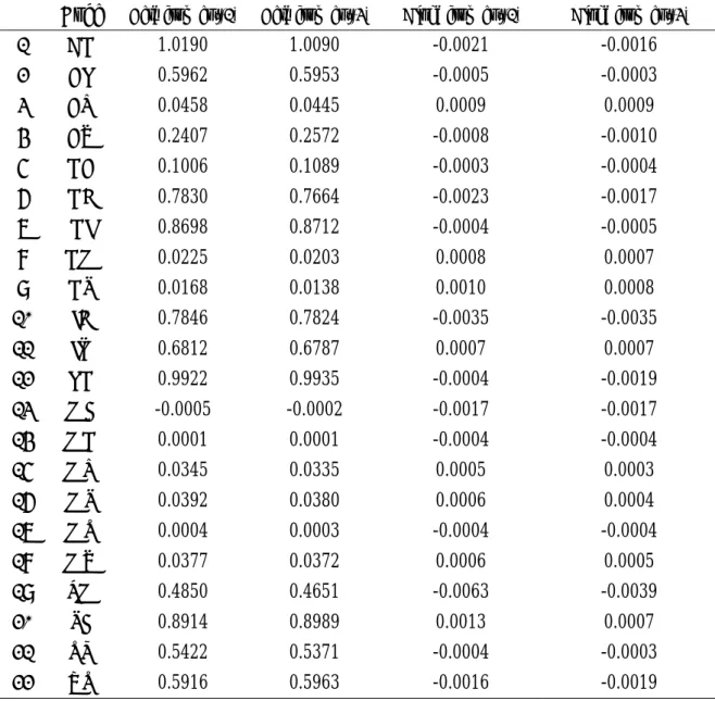
14 TABLE 2 – Beta and Alpha for Different Types of Mutual Funds

Code Beta from eq.(1) Beta from eq.(3) Alpha from eq.(1) Alpha from eq.(3)

1 AG 1.0190 1.0090 -0.0021 -0.0016 2 BL 0.5962 0.5953 -0.0005 -0.0003 3 BQ 0.0458 0.0445 0.0009 0.0009 4 BY 0.2407 0.2572 -0.0008 -0.0010 5 GB 0.1006 0.1089 -0.0003 -0.0004 6 GE 0.7830 0.7664 -0.0023 -0.0017 7 GI 0.8698 0.8712 -0.0004 -0.0005 8 GM 0.0225 0.0203 0.0008 0.0007 9 GS 0.0168 0.0138 0.0010 0.0008 10 IE 0.7846 0.7824 -0.0035 -0.0035 11 IN 0.6812 0.6787 0.0007 0.0007 12 LG 0.9922 0.9935 -0.0004 -0.0019 13 MF -0.0005 -0.0002 -0.0017 -0.0017 14 MG 0.0001 0.0001 -0.0004 -0.0004 15 MQ 0.0345 0.0335 0.0005 0.0003 16 MS 0.0392 0.0380 0.0006 0.0004 17 MT 0.0004 0.0003 -0.0004 -0.0004 18 MY 0.0377 0.0372 0.0006 0.0005 19 PM 0.4850 0.4651 -0.0063 -0.0039 20 SF 0.8914 0.8989 0.0013 0.0007 21 TR 0.5422 0.5371 -0.0004 -0.0003 22 UT 0.5916 0.5963 -0.0016 -0.0019

(15)

TABLE 3 – Functional Form Analyses for Different Types of Mutual Funds

Code NO. Not different from zero and one

Different from one and zero

Different from zero but not one

Different from one but not zero 1 AG 199 121 26 9 43 2 BL 77 61 9 4 3 3 BQ 221 214 6 0 1 4 BY 57 44 5 7 1 5 GB 48 33 15 0 0 6 GE 57 35 13 1 8 7 GI 200 119 45 20 16 8 GM 72 70 2 0 0 9 GS 138 138 0 0 0 10 IE 136 94 14 13 15 11 IN 59 38 14 5 2 12 LG 240 150 37 25 28 13 MF 217 216 1 0 0 14 MG 167 167 0 0 0 15 MQ 171 163 1 6 1 16 MS 413 393 3 16 1 17 MT 192 192 0 0 0 18 MY 19 17 1 1 0 19 PM 16 5 1 0 10 20 SF 84 57 11 3 13 21 TR 78 53 16 2 7 22 UT 22 17 0 5 0 Total 2883 2397 220 117 149

(16)

TABLE 4 – Summary Analysis of λ, α, and β

Mean Median Max. Min. Std. Dev. J-B 1 lambda 2.5080 4.1950 5.0000 -4.0000 2.9492 366.4 2 Absolute value of Lambda 3.4382 4.1950 5.0000 0.0000 1.7788 363.0 3 Beta from eq.(1) 0.3625 0.0492 1.9409 -0.9624 0.4448 382.9 4 Beta from eq.(3) 0.3615 0.0477 1.9988 -0.9933 0.4438 376.7 5 Ave. Market Elasticity 0.3639 0.0513 1.9473 -0.9503 0.4454 383.2 6 Alpha from eq.(1) -0.0004 0.0000 0.3513 -0.0367 0.0071 526000000.0 7 Alpha from eq.(3) -0.0005 -0.0001 0.0086 -0.0310 0.0025 61214.5 8 Difference in Beta [3-4] 0.0010 0.0005 0.1512 -0.1958 0.0200 36702.7 9 absolute diff. in Beta l3-4l 0.0090 0.0021 0.1958 0.0000 0.0179 51926.8 10 difference in alpha [6-7] 0.0001 0.0000 0.3538 -0.0067 0.0066 927000000.0 11 absolute diff. in alpha l6-7l 0.0005 0.0001 0.3538 0.0000 0.0066 940000000.0 12 Bias in using beta from eq.(3) -0.0857 -0.0388 158.4862 -180.1793 4.7414 162000000.0 Note: J-B represents Jarque-Bera

(17)

APPENDIX A

TABLE A-1

SUMMARY MEASURES OF AG

Mean Median Max. Min. Std. Dev. J-B 1 lambda 0.3121 -0.1500 5.0000 -3.6300 1.8666 10.1530 2 Absolute value of Lambda 1.4880 1.2500 5.0000 0.0200 1.1648 24.3627 3 Beta from eq.(1) 1.0190 1.0378 1.7523 -0.1256 0.3213 5.9753 4 Beta from eq.(3) 1.0090 1.0396 1.8792 -0.1266 0.3028 5.6975 5 Ave. Market Elasticity 1.0201 1.0380 1.7749 -0.1273 0.3207 5.9279 6 Alpha from eq.(1) -0.0021 -0.0020 0.0080 -0.0367 0.0057 1126.4820 7 Alpha from eq.(3) -0.0016 -0.0013 0.0066 -0.0310 0.0047 1620.8310 8 Difference in Beta [3-4] 0.0100 0.0041 0.1440 -0.1269 0.0394 2.7229 9 absolute diff. in Beta l3-4l 0.0317 0.0266 0.1440 0.0004 0.0255 76.0022 10 difference in alpha [6-7] -0.0005 -0.0001 0.0060 -0.0060 0.0018 8.4209 11 absolute diff. in alpha l6-7l 0.0014 0.0011 0.0060 0.0000 0.0012 89.4645 12 Bias in using beta from eq.(3) -0.0038 -0.0046 0.1678 -0.1064 0.0389 18.4222

TABLE A-2

SUMMARY MEASURES OF BL

Mean Median Max. Min. Std. Dev. J-B

1 lambda 1.42 1.76 5.00 -4.00 2.44 1.83

2 Absolute value of Lambda 2.32 1.90 5.00 0.08 1.59 5.96 3 Beta from eq.(1) 0.5962 0.5823 1.1372 0.3691 0.1236 67.3049 4 Beta from eq.(3) 0.5953 0.5779 1.0740 0.3637 0.1221 28.4918 5 Ave. Market Elasticity 0.5992 0.5855 1.1367 0.3716 0.1231 63.1351 6 Alpha from eq.(1) -0.0005 -0.0006 0.0035 -0.0058 0.0018 1.3785 7 Alpha from eq.(3) -0.0003 -0.0005 0.0038 -0.0038 0.0017 1.2638 8 Difference in Beta [3-4] 0.0009 0.0004 0.0633 -0.0369 0.0108 726.3556 9 absolute diff. in Beta l3-4l 0.0062 0.0043 0.0633 0.0001 0.0089 1752.1700 10 difference in alpha [6-7] -0.0002 -0.0001 0.0011 -0.0027 0.0005 394.4705

(18)

18 TABLE A-3

SUMMARY MEASURES OF GM

1 lambda 3.00 4.69 5.00 -4.00 2.70 65.83

2 Absolute value of Lambda 3.70 4.69 5.00 0.10 1.61 33.35 3 Beta from eq.(1) 0.0458 0.0360 0.3021 -0.0137 0.0470 1148.69 4 Beta from eq.(3) 0.0445 0.0318 0.2995 -0.0136 0.0485 1008.94 5 Ave. Market Elasticity 0.0468 0.0370 0.3008 -0.0136 0.0473 1047.54 6 Alpha from eq.(1) 0.0009 0.0009 0.0039 -0.0016 0.0006 67.03 7 Alpha from eq.(3) 0.0009 0.0008 0.0032 -0.0012 0.0006 23.69 8 Difference in Beta [3-4] 0.0013 0.0020 0.0081 -0.0329 0.0046 5833.31 9 absolute diff. in Beta l3-4l 0.0030 0.0024 0.0329 0.0000 0.0037 9283.05 10 difference in alpha [6-7] 0.0001 0.0000 0.0007 -0.0004 0.0001 997.86 11 absolute diff. in alpha l6-7l 0.0001 0.0001 0.0007 0.0000 0.0001 2564.54 12 Bias in using beta from eq.(3) -0.8873 -0.0850 3.7432 -180.1793 12.1226 435551.90

TABLE A-4

SUMMARY MEASURES OF BY

1 lambda 1.35 1.52 5.00 -4.00 2.90 3.66

2 Absolute value of Lambda 2.71 2.89 5.00 0.02 1.67 4.18 3 Beta from eq.(1) 0.2407 0.2392 0.3932 0.0767 0.0548 6.22 4 Beta from eq.(3) 0.2572 0.2586 0.3754 0.0834 0.0579 6.28 5 Ave. Market Elasticity 0.2444 0.2421 0.3905 0.0799 0.0548 6.52 6 Alpha from eq.(1) -0.0008 -0.0009 0.0019 -0.0049 0.0013 4.47 7 Alpha from eq.(3) -0.0010 -0.0010 0.0017 -0.0063 0.0014 19.33 8 Difference in Beta [3-4] -0.0165 -0.0115 0.0209 -0.0784 0.0221 3.05 9 absolute diff. in Beta l3-4l 0.0205 0.0160 0.0784 0.0002 0.0184 7.06 10 difference in alpha [6-7] 0.0002 0.0001 0.0014 -0.0001 0.0002 303.82 11 absolute diff. in alpha l6-7l 0.0002 0.0001 0.0014 0.0000 0.0002 385.49 12 Bias in using beta from eq.(3) 0.0533 0.0402 0.2431 -0.0581 0.0701 3.72

(19)

TABLE A-5

SUMMARY MEASURES OF GB

1 lambda 0.98 1.37 5.00 -4.00 3.92 6.4256

2 Absolute value of Lambda 3.73 4.00 5.00 0.29 1.45 7.0383 3 Beta from eq.(1) 0.1006 0.0836 0.2926 -0.4139 0.1409 78.9736 4 Beta from eq.(3) 0.1089 0.0851 0.4240 -0.4473 0.1617 44.0417 5 Ave. Market Elasticity 0.1035 0.0847 0.3057 -0.4088 0.1428 66.1191 6 Alpha from eq.(1) -0.0003 -0.0002 0.0032 -0.0062 0.0019 14.3871 7 Alpha from eq.(3) -0.0004 -0.0002 0.0030 -0.0043 0.0015 0.9261 8 Difference in Beta [3-4] -0.0083 -0.0003 0.0333 -0.1414 0.0325 253.9727 9 absolute diff. in Beta l3-4l 0.0144 0.0030 0.1414 0.0003 0.0302 311.4996 10 difference in alpha [6-7] 0.0001 0.0001 0.0023 -0.0029 0.0009 66.9274 11 absolute diff. in alpha l6-7l 0.0005 0.0002 0.0029 0.0000 0.0007 76.2673 12 Bias in using beta from eq.(3) 0.0129 -0.0004 0.6994 -0.2483 0.1617 116.7812

TABLE A-6

SUMMARY MEASURES OF GE

1 lambda -0.93 -1.13 4.17 -4.00 2.15 2.17

2 Absolute value of Lambda 1.97 1.69 4.17 0.04 1.25 4.12 3 Beta from eq.(1) 0.7830 0.8011 1.1007 0.2287 0.2154 4.80 4 Beta from eq.(3) 0.7664 0.7971 1.0702 0.2351 0.1953 6.28 5 Ave. Market Elasticity 0.7821 0.7999 1.0944 0.2267 0.2144 4.85 6 Alpha from eq.(1) -0.0023 -0.0017 0.0040 -0.0085 0.0033 3.06 7 Alpha from eq.(3) -0.0017 -0.0013 0.0037 -0.0078 0.0030 2.16 8 Difference in Beta [3-4] 0.0166 0.0045 0.0919 -0.0656 0.0350 2.50 9 absolute diff. in Beta l3-4l 0.0281 0.0192 0.0919 0.0002 0.0265 10.16 10 difference in alpha [6-7] -0.0006 -0.0001 0.0014 -0.0037 0.0011 11.74 11 absolute diff. in alpha l6-7l 0.0008 0.0004 0.0037 0.0000 0.0009 29.54

(20)

20 TABLE A-7

SUMMARY MEASURES OF GI

1 lambda 1.31 1.44 5.00 -4.00 2.53 8.35

2 Absolute value of Lambda 2.39 2.14 5.00 0.01 1.54 15.13 3 Beta from eq.(1) 0.8698 0.8755 1.6648 0.3029 0.1854 25.54 4 Beta from eq.(3) 0.8712 0.8806 1.7711 0.2910 0.1898 64.30 5 Ave. Market Elasticity 0.8721 0.8748 1.7164 0.3052 0.1868 43.72 6 Alpha from eq.(1) -0.0004 -0.0003 0.0071 -0.0183 0.0027 980.57 7 Alpha from eq.(3) -0.0005 -0.0004 0.0068 -0.0228 0.0029 3384.30 8 Difference in Beta [3-4] -0.0014 0.0008 0.0517 -0.1064 0.0151 2102.69 9 absolute diff. in Beta l3-4l 0.0089 0.0054 0.1064 0.0000 0.0123 5920.97 10 difference in alpha [6-7] 0.0001 0.0000 0.0046 -0.0023 0.0006 7993.08 11 absolute diff. in alpha l6-7l 0.0003 0.0001 0.0046 0.0000 0.0005 13268.77 12 Bias in using beta from eq.(3) -0.0016 -0.0007 0.0536 -0.0464 0.0143 42.71

TABLE A-8

SUMMARY MEASURES OF GM

1 lambda 3.28 5.00 5.00 -4.00 3.19 35.96

2 Absolute value of Lambda 4.44 5.00 5.00 0.17 1.05 151.23 3 Beta from eq.(1) 0.0225 0.0252 0.0602 -0.0093 0.0177 2.46 4 Beta from eq.(3) 0.0203 0.0228 0.0559 -0.0115 0.0168 2.24 5 Ave. Market Elasticity 0.0234 0.0264 0.0632 -0.0095 0.0184 2.37 6 Alpha from eq.(1) 0.0008 0.0009 0.0019 -0.0006 0.0006 2.14 7 Alpha from eq.(3) 0.0007 0.0008 0.0019 -0.0005 0.0005 1.62 8 Difference in Beta [3-4] 0.0022 0.0026 0.0072 -0.0066 0.0022 31.91 9 absolute diff. in Beta l3-4l 0.0027 0.0027 0.0072 0.0000 0.0016 1.97 10 difference in alpha [6-7] 0.0000 0.0000 0.0006 -0.0001 0.0001 534.55 11 absolute diff. in alpha l6-7l 0.0001 0.0000 0.0006 0.0000 0.0001 922.81 12 Bias in using beta from eq.(3) 0.1040 -0.1222 13.6552 -0.8718 1.7110 9264.16

(21)

TABLE A-9

SUMMARY MEASURES OF GS

1 lambda 2.85 5.00 5.00 -4.00 3.18 36.22

TABLE A-10

SUMMARY MEASURES OF IE

1 lambda -0.58 -0.66 3.90 -4.00 1.70 1.42

2 Absolute value of Lambda 1.48 1.34 4.00 0.02 1.01 12.10 3 Beta from eq.(1) 0.7846 0.7525 1.2122 0.3411 0.1634 7.99 4 Beta from eq.(3) 0.7824 0.7300 1.3391 0.3454 0.1838 36.99 5 Ave. Market Elasticity 0.7865 0.7501 1.2115 0.3397 0.1679 11.07 6 Alpha from eq.(1) -0.0035 -0.0035 0.0044 -0.0114 0.0033 0.36 7 Alpha from eq.(3) -0.0035 -0.0032 0.0046 -0.0123 0.0036 2.79 8 Difference in Beta [3-4] 0.0022 0.0061 0.1211 -0.1958 0.0454 188.22 9 absolute diff. in Beta l3-4l 0.0285 0.0172 0.1958 0.0001 0.0354 281.98 10 difference in alpha [6-7] 0.0000 -0.0003 0.0085 -0.0037 0.0020 201.11 11 absolute diff. in alpha l6-7l 0.0013 0.0006 0.0085 0.0000 0.0015 371.19

(22)

22 TABLE A-11

SUMMARY MEASURES OF IN

1 lambda 2.23 2.53 5.00 -3.09 2.37 4.32

2 Absolute value of Lambda 2.78 2.78 5.00 0.04 1.68 4.66 3 Beta from eq.(1) 0.6812 0.6876 1.0274 0.2657 0.1448 1.12 4 Beta from eq.(3) 0.6787 0.6833 0.9912 0.2538 0.1471 1.00 5 Ave. Market Elasticity 0.6838 0.6902 1.0261 0.2648 0.1447 1.28 6 Alpha from eq.(1) 0.0007 0.0004 0.0074 -0.0032 0.0022 10.42 7 Alpha from eq.(3) 0.0007 0.0007 0.0066 -0.0031 0.0020 3.42 8 Difference in Beta [3-4] 0.0025 0.0007 0.0858 -0.0259 0.0170 224.18 9 absolute diff. in Beta l3-4l 0.0101 0.0059 0.0858 0.0001 0.0139 548.87 10 difference in alpha [6-7] 0.0000 0.0000 0.0010 -0.0007 0.0003 17.81 11 absolute diff. in alpha l6-7l 0.0002 0.0001 0.0010 0.0000 0.0002 35.55 12 Bias in using beta from eq.(3) -0.0084 -0.0027 0.0326 -0.1196 0.0247 144.42

TABLE A-12

SUMMARY MEASURES OF LG

1 lambda 0.84 0.61 5.00 -3.93 2.19 7.95

2 Absolute value of Lambda 1.88 1.55 5.00 0.00 1.39 22.08 3 Beta from eq.(1) 0.9922 0.9923 1.7653 0.0432 0.2484 6.48 4 Beta from eq.(3) 0.9935 0.9964 1.8008 0.0407 0.2451 8.57 5 Ave. Market Elasticity 0.9948 0.9961 1.7730 0.0462 0.2489 6.34 6 Alpha from eq.(1) -0.0004 -0.0020 0.3513 -0.0227 0.0231 508535.80 7 Alpha from eq.(3) -0.0019 -0.0017 0.0065 -0.0234 0.0036 337.55 8 Difference in Beta [3-4] -0.0013 0.0002 0.1512 -0.0954 0.0279 254.60 9 absolute diff. in Beta l3-4l 0.0178 0.0104 0.1512 0.0000 0.0215 716.79 10 difference in alpha [6-7] 0.0016 0.0001 0.3538 -0.0057 0.0229 556550.60 11 absolute diff. in alpha l6-7l 0.0022 0.0004 0.3538 0.0000 0.0228 558523.30 12 Bias in using beta from eq.(3) -0.0002 -0.0002 0.1414 -0.1175 0.0261 467.38

(23)

TABLE A-13

SUMMARY MEASURES OF MF

1 lambda 3.82 5.00 5.00 -4.00 3.03 243.81

2 Absolute value of Lambda 4.85 5.00 5.00 0.83 0.43 10843.00 3 Beta from eq.(1) -0.0005 -0.0006 0.0037 -0.0024 0.0007 322.72 4 Beta from eq.(3) -0.0002 -0.0002 0.0043 -0.0022 0.0006 2303.45 5 Ave. Market Elasticity -0.0005 -0.0007 0.0036 -0.0026 0.0007 258.61 6 Alpha from eq.(1) -0.0017 -0.0017 -0.0012 -0.0021 0.0002 1.48 7 Alpha from eq.(3) -0.0017 -0.0018 -0.0013 -0.0021 0.0002 1.36 8 Difference in Beta [3-4] -0.0003 -0.0004 0.0005 -0.0007 0.0003 188.90 9 absolute diff. in Beta l3-4l 0.0004 0.0004 0.0007 0.0000 0.0001 30.41 10 difference in alpha [6-7] 0.0000 0.0000 0.0000 0.0000 0.0000 131.54 11 absolute diff. in alpha l6-7l 0.0000 0.0000 0.0000 0.0000 0.0000 7.91 12 Bias in using beta from eq.(3) -0.8130 -0.5568 10.4811 -17.2266 2.0807 7922.58

TABLE A-14

SUMMARY MEASURES OF MG

1 lambda 4.60 5.00 5.00 -4.00 1.83 2713.59

2 Absolute value of Lambda 4.93 5.00 5.00 0.82 0.38 50477.08 3 Beta from eq.(1) 0.0001 0.0002 0.0020 -0.0022 0.0004 538.72 4 Beta from eq.(3) 0.0001 0.0001 0.0020 -0.0024 0.0004 722.63 5 Ave. Market Elasticity 0.0001 0.0002 0.0020 -0.0022 0.0004 436.90 6 Alpha from eq.(1) -0.0004 -0.0004 0.0000 -0.0012 0.0002 1.08 7 Alpha from eq.(3) -0.0004 -0.0004 0.0000 -0.0012 0.0002 1.12 8 Difference in Beta [3-4] 0.0000 0.0000 0.0003 -0.0002 0.0001 38.14 9 absolute diff. in Beta l3-4l 0.0001 0.0000 0.0003 0.0000 0.0001 136.92 10 difference in alpha [6-7] 0.0000 0.0000 0.0000 0.0000 0.0000 382.90 11 absolute diff. in alpha l6-7l 0.0000 0.0000 0.0000 0.0000 0.0000 1220.99

(24)

24 TABLE A-15

SUMMARY MEASURES OF MQ

1 lambda 4.45 5.00 5.00 -4.00 1.61 1546.48

TABLE A-16

SUMMARY MEASURES OF MS

1 lambda 4.61 5.00 5.00 -4.00 1.40 13395.08

(25)

TABLE A-17

SUMMARY MEASURES OF MT

1 lambda 4.13 5.00 5.00 -4.00 2.65 463.06

2 Absolute value of Lambda 4.88 5.00 5.00 1.50 0.40 7207.87 3 Beta from eq.(1) 0.0004 0.0004 0.0023 -0.0073 0.0008 18622.09 4 Beta from eq.(3) 0.0003 0.0003 0.0020 -0.0061 0.0007 9791.87 5 Ave. Market Elasticity 0.0004 0.0004 0.0024 -0.0077 0.0008 19742.25 6 Alpha from eq.(1) -0.0004 -0.0004 0.0001 -0.0016 0.0002 187.29 7 Alpha from eq.(3) -0.0004 -0.0004 0.0001 -0.0016 0.0002 198.33 8 Difference in Beta [3-4] 0.0000 0.0000 0.0003 -0.0012 0.0001 20286.67 9 absolute diff. in Beta l3-4l 0.0001 0.0000 0.0012 0.0000 0.0001 40705.30 10 difference in alpha [6-7] 0.0000 0.0000 0.0001 0.0000 0.0000 50860.04 11 absolute diff. in alpha l6-7l 0.0000 0.0000 0.0001 0.0000 0.0000 99049.90 12 Bias in using beta from eq.(3) -0.2288 -0.0953 2.9890 -22.9903 1.8230 133309.90

TABLE A-18

SUMMARY MEASURES OF MY

1 lambda 4.88 5.00 5.00 3.11 0.44 167.21

2 Absolute value of Lambda 4.88 5.00 5.00 3.11 0.44 167.21 3 Beta from eq.(1) 0.0377 0.0379 0.0513 0.0102 0.0098 4.29 4 Beta from eq.(3) 0.0372 0.0375 0.0494 0.0098 0.0096 5.59 5 Ave. Market Elasticity 0.0394 0.0397 0.0524 0.0107 0.0102 4.71 6 Alpha from eq.(1) 0.0006 0.0006 0.0013 -0.0004 0.0005 1.17 7 Alpha from eq.(3) 0.0005 0.0005 0.0011 -0.0005 0.0004 1.58 8 Difference in Beta [3-4] 0.0005 0.0007 0.0019 -0.0008 0.0008 0.50 9 absolute diff. in Beta l3-4l 0.0008 0.0008 0.0019 0.0001 0.0005 0.96 10 difference in alpha [6-7] 0.0001 0.0001 0.0002 0.0000 0.0001 1.13 11 absolute diff. in alpha l6-7l 0.0001 0.0001 0.0002 0.0000 0.0001 1.13

(26)

26 TABLE A-19

SUMMARY MEASURES OF PM

1 lambda -0.61 -0.69 0.55 -1.41 0.53 0.80

2 Absolute value of Lambda 0.70 0.69 1.41 0.06 0.40 0.32 3 Beta from eq.(1) 0.4850 0.4891 0.6075 0.3335 0.0872 1.14 4 Beta from eq.(3) 0.4651 0.4502 0.6051 0.3245 0.0897 0.97 5 Ave. Market Elasticity 0.4849 0.4888 0.6079 0.3325 0.0879 1.13 6 Alpha from eq.(1) -0.0063 -0.0059 -0.0012 -0.0147 0.0037 2.35 7 Alpha from eq.(3) -0.0039 -0.0022 -0.0005 -0.0121 0.0035 3.94 8 Difference in Beta [3-4] 0.0199 0.0210 0.0621 -0.0216 0.0197 0.06 9 absolute diff. in Beta l3-4l 0.0233 0.0220 0.0621 0.0027 0.0152 2.40 10 difference in alpha [6-7] -0.0024 -0.0026 0.0026 -0.0067 0.0023 0.35 11 absolute diff. in alpha l6-7l 0.0029 0.0027 0.0067 0.0003 0.0017 0.71 12 Bias in using beta from eq.(3) -0.0420 -0.0445 0.0292 -0.1170 0.0369 0.03

TABLE A-20

SUMMARY MEASURES OF SF

1 lambda 0.55 0.33 5.00 -4.00 1.89 0.49

2 Absolute value of Lambda 1.49 1.13 5.00 0.04 1.27 12.28 3 Beta from eq.(1) 0.8914 0.7790 1.9409 0.2228 0.4053 17.91 4 Beta from eq.(3) 0.8989 0.7752 1.9988 0.2092 0.4159 18.55 5 Ave. Market Elasticity 0.8935 0.7833 1.9473 0.2234 0.4055 17.98 6 Alpha from eq.(1) 0.0013 0.0013 0.0108 -0.0090 0.0041 0.71 7 Alpha from eq.(3) 0.0007 0.0015 0.0086 -0.0141 0.0038 35.94 8 Difference in Beta [3-4] -0.0075 -0.0020 0.0642 -0.1352 0.0273 145.65 9 absolute diff. in Beta l3-4l 0.0168 0.0083 0.1352 0.0003 0.0228 326.91 10 difference in alpha [6-7] 0.0006 0.0003 0.0068 -0.0038 0.0019 7.59 11 absolute diff. in alpha l6-7l 0.0015 0.0010 0.0068 0.0000 0.0014 47.02 12 Bias in using beta from eq.(3) 0.0019 0.0010 0.1275 -0.1057 0.0323 75.70

(27)

TABLE A-21

SUMMARY MEASURES OF TR

1 lambda -0.24 -0.67 5.00 -4.00 2.67 4.21

2 Absolute value of Lambda 2.29 1.98 5.00 0.02 1.37 5.29 3 Beta from eq.(1) 0.5422 0.5898 1.2131 -0.9624 0.3238 400.81 4 Beta from eq.(3) 0.5371 0.5926 1.1964 -0.9933 0.3261 437.33 5 Ave. Market Elasticity 0.5433 0.5943 1.2102 -0.9503 0.3221 394.67 6 Alpha from eq.(1) -0.0004 -0.0002 0.0040 -0.0082 0.0021 33.04 7 Alpha from eq.(3) -0.0003 -0.0003 0.0045 -0.0074 0.0018 15.52 8 Difference in Beta [3-4] 0.0051 0.0023 0.0453 -0.0167 0.0125 25.92 9 absolute diff. in Beta l3-4l 0.0089 0.0052 0.0453 0.0001 0.0102 69.19 10 difference in alpha [6-7] -0.0002 0.0000 0.0011 -0.0030 0.0006 314.13 11 absolute diff. in alpha l6-7l 0.0004 0.0002 0.0030 0.0000 0.0005 821.59 12 Bias in using beta from eq.(3) -0.0097 -0.0067 0.0463 -0.1248 0.0260 96.10

TABLE A-22

SUMMARY MEASURES OF UT

1 lambda 0.91 0.12 3.44 -1.52 1.47 1.93

2 Absolute value of Lambda 1.22 0.58 3.44 0.01 1.22 2.61 3 Beta from eq.(1) 0.5916 0.5265 1.3532 0.1456 0.2571 9.96 4 Beta from eq.(3) 0.5963 0.5258 1.3435 0.1363 0.2648 8.05 5 Ave. Market Elasticity 0.5949 0.5262 1.3520 0.1473 0.2590 9.20 6 Alpha from eq.(1) -0.0016 -0.0013 0.0018 -0.0065 0.0021 2.87 7 Alpha from eq.(3) -0.0019 -0.0014 0.0009 -0.0079 0.0022 5.70 8 Difference in Beta [3-4] -0.0047 -0.0003 0.0097 -0.0690 0.0172 72.36 9 absolute diff. in Beta l3-4l 0.0087 0.0021 0.0690 0.0001 0.0154 104.04 10 difference in alpha [6-7] 0.0003 0.0000 0.0018 -0.0004 0.0006 5.14 11 absolute diff. in alpha l6-7l 0.0004 0.0001 0.0018 0.0000 0.0005 9.34

(28)

28 Appendix B

Table B-1

DISTRIBUTION FOR THE FUNCTIONAL FORM PARAMETER LAMBDA OF AG Optimal LD NO. Not different from zero and one Different from one and zero Different from zero but not one

Different from one but not zero -5 0 0 0 0 0 -4.99 to -4.00 0 0 0 0 0 -3.99 to -3.00 4 0 4 0 0 -2.99 to -2.00 12 0 8 0 4 -1.99 to -1.00 35 3 8 0 24 -0.99 to -0.50 28 13 1 0 14 -0.49 to -0.01 26 24 1 0 1 0 0 0 0 0 0 0.01 to 0.49 20 20 0 0 0 0.50 to 0.99 10 10 0 0 0 1.00 to 1.99 22 21 0 1 0 2.00 to 2.99 14 12 0 2 0 3.00 to 3.99 24 18 0 6 0 4.00 to 4.99 1 0 1 0 0 5.00 3 0 3 0 0 Total 199 121 26 9 43

(29)

Table B-2

DISTRIBUTION FOR THE FUNCTIONAL FORM PARAMETER LAMBDA OF BL Optimal LD NO. Not different from zero and one Different from one and zero Different from zero but not one

Different from one but not zero

-5 0 0 0 0 0 -4.99 to -4.00 2 0 2 0 0 -3.99 to -3.00 2 1 0 0 1 -2.99 to -2.00 2 1 0 0 1 -1.99 to -1.00 5 4 0 0 1 -0.99 to -0.50 7 7 0 0 0 -0.49 to -0.01 6 6 0 0 0 0 0 0 0 0 0 0.01 to 0.49 6 6 0 0 0 0.50 to 0.99 0 0 0 0 0 1.00 to 1.99 18 18 0 0 0 2.00 to 2.99 9 9 0 0 0 3.00 to 3.99 6 5 0 1 0 4.00 to 4.99 3 1 2 0 0 5.00 11 3 5 3 0 Total 77 61 9 4 3

(30)

30 Table B-3

DISTRIBUTION FOR THE FUNCTIONAL FORM PARAMETER LAMBDA OF BQ Optimal LD NO. Not different from zero and one Different from one and zero Different from zero but not one

(31)

Table B-4

DISTRIBUTION FOR THE FUNCTIONAL FORM PARAMETER LAMBDA OF BY Optimal LD NO. Not different from zero and one Different from one and zero Different from zero but not one

(32)

32 Table B-5

DISTRIBUTION FOR THE FUNCTIONAL FORM PARAMETER LAMBDA OF GB Optimal LD NO. Not different from zero and one Different from one and zero Different from zero but not one

(33)

Table B-6

DISTRIBUTION FOR THE FUNCTIONAL FORM PARAMETER LAMBDA OF GE Optimal LD NO. Not different from zero and one Different from one and zero Different from zero but not one

(34)

34 Table B-7

DISTRIBUTION FOR THE FUNCTIONAL FORM PARAMETER LAMBDA OF GI Optimal LD NO. Not different from zero and one Different from one and zero Different from zero but not one

(35)

Table B-8

DISTRIBUTION FOR THE FUNCTIONAL FORM PARAMETER LAMBDA OF GM Optimal LD NO. Not different from zero and one Different from one and zero Different from zero but not one

(36)

36 Table B-9

DISTRIBUTION FOR THE FUNCTIONAL FORM PARAMETER LAMBDA OF GS Optimal LD NO. Not different from zero and one Different from one and zero Different from zero but not one

(37)

Table B-10

DISTRIBUTION FOR THE FUNCTIONAL FORM PARAMETER LAMBDA OF IE Optimal LD NO. Not different from zero and one Different from one and zero Different from zero but not one

(38)

38 Table B-11

DISTRIBUTION FOR THE FUNCTIONAL FORM PARAMETER LAMBDA OF IN Optimal LD NO. Not different from zero and one Different from one and zero Different from zero but not one

(39)

Table B-12

DISTRIBUTION FOR THE FUNCTIONAL FORM PARAMETER LAMBDA OF LG Optimal LD NO. Not different from zero and one Different from one and zero Different from zero but not one

(40)

40 Table B-13

DISTRIBUTION FOR THE FUNCTIONAL FORM PARAMETER LAMBDA OF MF Optimal LD NO. Not different from zero and one Different from one and zero Different from zero but not one

(41)

Table B-14

DISTRIBUTION FOR THE FUNCTIONAL FORM PARAMETER LAMBDA OF MG Optimal LD NO. Not different from zero and one Different from one and zero Different from zero but not one

(42)

42 Table B-15

DISTRIBUTION FOR THE FUNCTIONAL FORM PARAMETER LAMBDA OF MQ Optimal LD NO. Not different from zero and one Different from one and zero Different from zero but not one

(43)

Table B-16

DISTRIBUTION FOR THE FUNCTIONAL FORM PARAMETER LAMBDA OF MS Optimal LD NO. Not different from zero and one Different from one and zero Different from zero but not one

(44)

44 Table B-17

DISTRIBUTION FOR THE FUNCTIONAL FORM PARAMETER LAMBDA OF MT Optimal LD NO. Not different from zero and one Different from one and zero Different from zero but not one

(45)

Table B-18

DISTRIBUTION FOR THE FUNCTIONAL FORM PARAMETER LAMBDA OF MY Optimal LD NO. Not different from zero and one Different from one and zero Different from zero but not one

(46)

46 Table B-19

DISTRIBUTION FOR THE FUNCTIONAL FORM PARAMETER LAMBDA OF PM Optimal LD NO. Not different from zero and one Different from one and zero Different from zero but not one

(47)

Table B-20

DISTRIBUTION FOR THE FUNCTIONAL FORM PARAMETER LAMBDA OF SF Optimal LD NO. Not different from zero and one Different from one and zero Different from zero but not one

(48)

48 Table B-21

DISTRIBUTION FOR THE FUNCTIONAL FORM PARAMETER LAMBDA OF TR Optimal LD NO. Not different from zero and one Different from one and zero Different from zero but not one

(49)

Table B-22

DISTRIBUTION FOR THE FUNCTIONAL FORM PARAMETER LAMBDA OF UT Optimal LD NO. Not different from zero and one Different from one and zero Different from zero but not one

(50)

50

Part Two: 台灣與美國共同基金績效分析之比較

A Comparison between Taiwan and U.S. Mutual Fund Performance

本部分研究成果已編輯為國立交通大學財務金融所九十三年六月畢業之黃曉芸同學碩士

論文，詳細內容可於網上查詢，其摘要及目錄如下:

研究生：黃曉芸 (Shiao-Yun Huang)

指導教授：李正福教授、林建榮教授 (Dr. Cheng-few Lee & Dr. Jian-rung Lin) 摘要: 國內論文探討共同基金績效的不下少數，但由於資料蒐集或變數處理上的問題，都只侷限在單一市場（台灣或美國）之探討，較少同時研究兩國或多國共同基金表現之文章。這使得國內研究若想與國外實證比較時，就只能參考過去的文獻。因此，本研究以台灣及美國開放式股票型基金為研究主題。藉由選用同樣的樣本期間與模型，討論兩個發展迥異市場中的共同基金整體績效表現、選股能力及擇時能力之差異。實證結果驗證了，股票市場組成結構會造成同樣是共同基金，但處於不同之國家，整體績效表現就會不同。台灣股市以散戶為主，對擁有較多資訊的法人來說，打敗市場並非難事。美國股市則以法人為主，所以僅有少數基金之表現可以超越市場。選股能力部分，台灣共同基金幾乎不存在著選股能力，甚至出現一些反向的選股能力。相反的，擇時能力幾乎是美國基金的基本配備。三年期與五年期下大概有四分之一的基金具有此項能力，十年期之實證結果也有十分之一的基金有之。擇時能力部分，台灣雖然只有少數基金具備擇時能力，但卻無基金會因錯估大盤走勢而作出錯誤的風險調整。然而，美國雖然有擇時能力之基金在絕對數量上與台灣差不多，但相對佔樣本之比例就小很多。此外，經理人對大盤錯估情形相當嚴重(在五年期實證結果發現的，三年期並不存在)。因此，在擇時能力之衡量上台灣基金是表現的比美國好的。關鍵字：台灣、美國、共同基金、整體績效、選股能力、擇時能力

(51)

Abstract:

The investment performance of mutual fund has been extensively studies in the finance literature. Because of the problems about data collection and variables treatment, few of researches analysed two national mutual fund performance at the same time. If we want to compare domestic empirical results with other countries, we just consult references. So, this study uses the same sample periods and the same models to examine empirically differences of overall performance, selectivity ability, and market-timing ability of equity funds between two markets which developed so differently, Taiwan and the United States.

Results indicated that composition of stock market could affect performance of mutual fund. Taiwan stock market was mainly composed of individual investors. So, institution

investors (mutual funds) which have superior information would beat market index easily. Few mutual funds took advantage over market in American because U.S. stock market was mainly composed of institution investors.Regarding selectivity ability, Taiwan mutual funds didn’t have positive selectivity ability, but some had negative selectivity ability. On the contrary, selectivity ability was the U.S. mutual fund’s basic outfit. One-fourth mutual funds had this ability in the three-year-period and five-year-period results. One-tenth mutual funds had this ability in the ten-year-period result. Regarding market-timing ablility, a small number of Taiwan mutual funds had positive market-timing ability. No Taiwan mutual funds made inappropriate risk adjustment because of wrong forcast of market movement. Although the absolute amount of U.S. mutual funds and Taiwan mutual funds which have positive

market-timing ability was the same, U.S. mutual funds took less proportion of sample relatively. Futhermore, U.S. mutual fund managers seriously forcasted market movement incorrectly. (demonstrated in five-year-period result) Hence,Taiwan mutual fund performed better than U.S. mutual funds with regard to market-timing ability.

Key word:Taiwan, the United States, Mutual Fund, Overall Performance, Selectivity Ability, Market-Timing Ability

52 1.2 研究目的……… 2 1.3 研究架構……… 3 二、文獻回顧……… 5 2.1 美國與台灣共同基金……… 5 2.1.1 共同基金之發展……… 5 2.1.2 共同基金之現況……… 8 2.2 共同基金績效評估模型之相關文獻……… 11 三、研究方法……… 17 3.1 研究範圍與資料來源……… 17 3.2 研究變數之定義……… 17 3.3 實證模型之構建……… 21 四、實證結果之分析……… 28 4.1 整體績效評估……… 28 4.2 選股能力與擇時能力評估……… 30 4.2.1 Jensen 指標……… 31 4.2.2 Treynor&Mazuy 模型……… 32 4.2.3 Henriksson&Merton 模型……… 34 4.2.4 Lee＆Rahman 模型……… 36 4.3 選股能力與擇時能力模型實證結果之綜合比較……… 38 五、結論與建議……… 41 5.1 結論……… 41 5.2 建議……… 43 參考文獻 ……… 45 附錄一台灣共同基金樣本明細……… 48 附錄二美國共同基金樣本明細……… 50

表目錄

表 2-1-1 臺灣基金淨資產總額與個數之成長情況……… 7 表 2-1-2 美國共同基金類型與各類型基金數量、規模及受益人數……… 9 表 2-1-3 台灣共同基金類型與各類型基金數量、規模及受益人數……… 11 表 4-1-1 台灣與美國三年期之 Treynor 指標及 Sharp 指標實證結果………… 28 表 4-1-2 台灣與美國五年期之 Treynor 指標及 Sharp 指標實證結果………… 29 表 4-1-3 美國十年期之 Treynor 指標及 Sharp 指標實證結果……… 29 表 4-2-1 台灣與美國 Jensen 指標之敘述統計……… 31 表 4-2-2 台灣與美國 Jensen 指標之正負值及顯著個數比較……… 31 表 4-2-3 台灣與美國之 Treynor&&Mazuy 模型敘述統計……… 33 表 4-2-4 台灣與美國 Treynor&&Mazuy 模型之

α

正負值及顯著個數比較…… 34 表 4-2-5 台灣與美國 Treynor&&Mazuy 模型之

β

₂正負值及顯著個數比較…… 34 表 4-2-6 台灣與美國 Henrisksson&Merton 模型敘述統計……… 35 表 4-2-7 台灣與美國 Henrisksson&Merton 模型

α

正負值及顯著個數比較… 35 表 4-2-8 台灣與美國 Henrisksson&Merton 模型

β

₂正負值及顯著個數比較… 35