應用於超寬頻系統之橫向電磁波號角天線

全文

(1)國立交通大學電信工程學系碩士班碩士論文應用於超寬頻系統之橫向電磁波號角天線. A TEM Horn Antenna for Ultra-wideband Applications. 研究生: 林昭男指導教授: 彭松村博士黃瑞彬博士. 中華民國九十三年七月.

(2) 應用於超寬頻系統中之橫電磁波號角天線 A TEM Horn Antenna for Ultra-wideband Applications 研究生：林昭男. Student: Chou-Nan Lin. 指導教授：彭松村博士. Advisor: Dr. Song-Tsuen Peng. 黃瑞彬博士. Dr. Ruey-Bing Hwang. 國立交通大學電信工程學系碩士班碩士論文. A Thesis Submitted to Institute of Communication Engineering College of Electrical Engineering and Computer Science National Chiao Tung University In Partial Fulfillment of the Requirements for the Degree of Master of Science In Communication Engineering July 2004 HsinChu, Taiwan, Republic of China 中華民國九十三年七月.

(3) 應用於超寬頻系統之橫向電磁波號角天線. 研究生: 林昭男. 指導教授: 彭松村教授黃瑞彬教授. 國立交通大學電信工程學系碩士班. 摘. 要. 在此篇論文中，我們使用了二種工具，其一為基於有限元素分析法之Ansoft HFSSTM來做嚴謹之全波模擬分析，另一則為根據孔徑上電場分佈之經驗公式所使用之等效原則來設計並完成應用於超寬頻系統中之橫電磁波號角電線。此天線結構是由兩片三角形且相距高度並非均勻之金屬板所組成。由於此結構可視為在長度及寬度方向皆漸層變化之平行板傳輸線，因此傳輸線模型可用來算出阻抗特性之起始值。除此之外，由於全波模擬所耗費過多的時間，因此我們僅在觀察其寬頻特性時使用它。然而，輻射場形則根據其孔徑上電場分佈之經驗公式，再藉由等效原理來算出。為了描繪這此種天線之輻射特性，我們改變了一些結構上的參數例如天線長度以及展開角來觀察其影響。一般來說，3-dB波束寬會隨著孔徑大小的增加而減小。除此之外，如同所觀察到的，平緩的漸層轉換結構可改善高頻之回波損耗。由於此天線具有易於製造，良好之輻射及頻寬的特性，因此預期將來可廣泛用於無線寬頻系統中最後一哩的應用。. I.

(4) A TEM Horn Antenna for Ultra-wideband Applications Student:. Chou-Nan Lin. Advisor:. Dr. Song-Tsuen Peng Dr. Ruey-Bing Hwang. Institute of Communication Engineering National Chiao Tung University. Abstract. In this thesis, we have employed the rigorous full-wave analysis Ansoft HFSSTM, based on the finite element method, and the equivalent principle, on the basis of empirical formula for the aperture field distribution, to design and implement the TEM horn antenna for ultra wideband applications. The structure under consideration is made up of two metallic triangular plates separated by a non-uniform distance. Since the structure can be considered as a parallel-plate waveguide with taper transition along its length and width directions both, the transmission line model could be utilized to figure out the impedance characteristics in the initial design. Besides, due to the excessive time consuming for the full-wave simulation, it is only used for examining its wideband characteristics, however, the radiation pattern is calculated by mean of equivalent principle with respect to its aperture field based on empirical formula. To characterize the radiation behavior of such a kind of antenna, we have changed some structural parameters, such as the length and the flare angle between the two metal plates. In general, the 3-dB beam-width decreases as the increase in the aperture size. Moreover, the smooth taper transition could improve the return loss in the high frequency range, as being confirmed by intuition. Since this antenna is simple in its fabrication and fairly good performance in its radiation and band width characteristics, it promises to be widespread employed in last mile applications for wireless communication systems.. II.

(5) 誌. 謝. 首先要感謝二位指導教授彭松村博士以及黃瑞彬博士在這二年中悉心地指導與鼓勵，讓我在微波領域方面的知識獲益良多，並且使得這篇論文能夠順利完成。同時也要感謝實驗室的學長以及同窗好友們，實驗室和諧的氣氛讓大家都能夠互相討論與學習，藉此時常能夠得到不同的觀點並對研究過程中所遇到的瓶頸有非常大的幫助。最後要感謝我的家人以及乾媽，由於他們的付出與關懷，讓我能夠毫無後顧之憂地學習，謹將此篇論文獻給他們。. III.

(6) Contents Chinese Abstract. Ⅰ. Abstract. Ⅱ. Acknowledgement. Ⅲ. Contents. Ⅳ. List of Figures. Ⅵ. List of Tables. Ⅷ. Chapter 1 Introduction. 1. Chapter 2 Theoretical Analysis. 3. 2.1 Equivalent Sources of TEM Horn Antenna. 3. 2.2 Radiation Far Field Pattern Calculation by Using Equivalent. 5. Principle 2.3Far Field Radiation Pattern. 7. 2.4Numerical Analysis. 8. 2.5Numerical Results. 9. Chapter 3 Design and Measurement. 13. 3.1Operation Principle. 13. 3.2Design Considerations. 14. 3.3Design Procedure. 15. 3.4 Full Wave Simulation of TEM Horn Antennas. 19. 3.5 Fabrication and Measurement. 20. Chapter 4 Variation of Parameters. 29 29. 4.1 Motivation. IV.

(7) 4.2 Design Considerations. 30. 4.3 Effect of Antenna Length on The Radiation Characteristics. 31. 4.4 Effect of Flare Angle on The Radiation Characteristics. 32. Chapter 5 Conclusion. 42. References. 44. V.

(8) List of Figures 2.1. Antenna structure. 4. 2.2. Actual and equivalent problem model. 6. 2.3. Computed H-plane pattern for constant length and different flare angles. 11. 2.4. Computed H-plane pattern for constant flare angle and different lengths. 12. 3.1. Structure of the linearly tapered TEM horn. 16. 3.2. Staircase model of TEM horn. 18. 3.3. Distribution of return loss against frequency for both measured and calculated results of the antenna based on Table 3.1. 22. 3.4. The fabricated TEM horn antenna. 23. 3.5. Distribution of return loss against frequency for both measured and calculated results of the antenna added with taper transition. 3.6. The measured and calculated H-plane radiation pattern of the TEM horn at 5 GHZ. 3.7. 26. The measured and calculated H-plane radiation pattern of the TEM horn at 7 GHZ. 3.8. 27. The measured and calculated H-plane radiation pattern of the TEM horn at 9 GHZ. 4.1. 28. Measured return loss for antennas with fixed flare angle α = 40° and three different antenna lengths. 4.2. 34. Measured and calculated H-plane patterns with α = 30° and L=50mm at 7GHz. 4.3. 35. Measured and calculated H-plane patterns with α = 30° and L=75mm at 7GHz. 4.4. 24. 36. Measured and calculated H-plane patterns with α = 30° and L=100mm at 7GHz. 37. VI.

(9) 4.5. Measured and calculated H-plane patterns with α = 45° and L=100mm at 7GHz. 4.6. 38. Measured and calculated H-plane patterns with α = 60° and L=100mm at 7GHz. 4.7. 39. 3dB beamwidth in H-plane of TEM horn antennas as a function of flare angle with a given antenna length L=100mm. 4.8. 40. 3dB beamwidth in H-plane of TEM horn antennas as a function of flare angle for different lengths. 41. VII.

(10) List of Tables 3.1. Antenna dimensions. 20. 3.2. Antenna dimensions added with taper transition. 21. VIII.

(11) Chapter 1 Introduction. Recently, ultra-wideband antennas that can operate over a very wide bandwidth have received increasing attention and interest for use in radar and communication systems in both military and civilian applications, such as satellite communication and mine detection. The FCC defines the ultra-wideband device as any device having a fractional bandwidth greater than 0.2 or 500 MHz spectrum range. An ultra-wideband system requires an antenna capable of receiving all frequencies at the same time. Thus, antenna behavior and performance must be consistent over entire band. Ideally, radiation pattern and impedance matching should be stable over the entire band.. Some wideband antennas have been developed for many years, such as bow tie, log-periodic, spiral, and transverse electromagnetic (TEM) horn antenna. However, the TEM horn antenna is probably the most commonly used antenna for UWB radar systems because of its high gain, wide band, and unidirectional radiation. These properties are especially significant for applications such as mine detection that need to overcome the high loss under ground.. 1.

(12) The conventional design of the TEM horn is on the basis of infinitely long biconical antennas. There are many variations of them including resistive loading, tapering the antenna plates, or placing a dielectric lens at the aperture, etc. Conventional TEM horn, in its simplest form, consists of two triangular metal plates. The planes of these triangles are separated by the flare angle α . The antenna is fed through a parallel plate transmission line connected at the apex. This type of configuration has the advantage of easy fabrication. Although many efforts have been made on TEM horn antennas, there are few published papers or documents focusing on the design procedure of this type antenna. In this thesis, we intent to develop an engineering design criterion base on numerical computation to fabricate a TEM horn antenna subject to the prescribed bandwidth and radiation characteristic. The design goal in this thesis is to obtain an ultra-wideband TEM horn antenna operating from 3.1 GHz to 10.6 GHz with high directivity in order to meet the requirement in IEEE 802.15.3a application.. 2.

(13) Chapter 2 Theoretical Analysis. 2.1 Equivalent sources of TEM Horn Antenna. In this section, we set a theoretical basis to predict the radiation characteristic of a TEM horn antenna. The structure under consideration is a pair of triangular conductor plates, which separated by a flare angle denoted as α . The antenna is fed with a parallel plate transmission line. Such a structure can be considered as the extension of a parallel two wire transmission line. Therefore, in the beginning of this analysis, it is assumed that the TEM horn mainly guide the TEM wave, by properly choosing the horn flare angle and the plate widths. To simplify the analysis, the edge diffraction effect and fringing fields were neglected. Then the fields over the aperture of the TEM horn antenna are assumed to be linearly polarized spherical waves.. As coordinate system attached in Fig. 2.2, the far field radiation can be regarded as that from a reference point, so called, phase center. Then the r0 represents the distance between the center of aperture and this reference point. The aperture fields can be expressed as. E y ( x' , y ' ,0) =. r0. 2. r0 + x' 2 + y ' 2 2. ⋅. e. − jk ( r0 2 + x '2 + y '2 − r0 ). (2.1). r0 + y ' 2 2. 3.

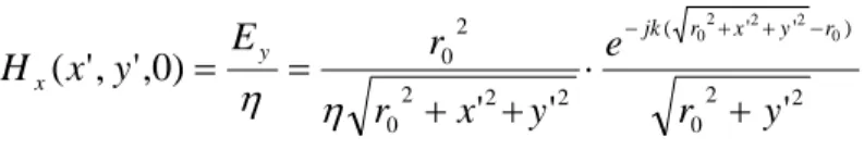
(14) H x ( x' , y ' ,0) =. Ey. η. =. r0. 2. η r0 2 + x' 2 + y ' 2. ⋅. e. − jk ( r0 2 + x '2 + y '2 − r0 ). (2.2). r0 + y ' 2 2. Where x' , y ' and z ' represent source point. η is the intrinsic impedance of TEM wave in free space. (a) 3D structure. (b) Top view. Fig. 2.1 Antenna structure. To develop an equivalent process for the original problem, it is necessary that the tangential electric and magnetic field components over a closed surface are known. The closed surface is chosen which extends to infinity on the x-y plane that coincides with the aperture of the horn. The difficulty encountered in this equivalent problem is that both E t and H t (along with their corresponding J s and M s ) are not zero outside the aperture and are also unknown there. By using the equivalent principle, we could assume that the electric and magnetic fields vanish inside the prescribed outer surface. Therefore, the equivalent electric and magnetic currents are impressed on the artificial surface, that is;. 4.

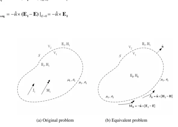
(15) J S eq = nˆ × H t (2.3) M S eq = E t × nˆ. Where E t and H t are those over the aperture of the antenna. Since the aperture fields have been well approximated by those demonstrated in the previous section, after substituting them into (2.3), the equivalent sources are given below:. J S = − aˆ y. M S = aˆ x. r02. η r02 + x' 2 + y' 2 r02 + y' 2 r02 r + x' + y' 2 0. 2. 2. r + y' 2 0. 2. e. e. − jk ( r02 + x '2 + y '2 − r0 ). − jk ( r02 + x '2 + y '2 − r0 ). (2.4). (2.5). 2.2 Radiation far field pattern calculation by using equivalent principle. The equivalence principle [2] is based on the uniqueness theorem which states that if the tangential component of electric or magnetic fields are specified over boundaries then the fields within it can be uniquely determined. As shown in Fig. 2.2(a), we consider the actual radiating source, which is represented by current densities J1 and M1. The sources will radiate fields E1 and H1 everywhere. If we would have the fields outside a certain closed surface as shown in dashed line, we could put equivalent sources on the boundary to obtain the same fields distribution as those in the original problem. To achieve it, we choose a closed surface S which encloses the real sources with current densities J1 and M1. We denote the volume within S by V1 and outside S by V2. Then an equivalent problem of Fig. 2.2(a) can be represented as shown in Fig. 2.1(b). The original sources J1 and M1 are removed, and the. 5.

(16) fields outside of S are E1 and H1. By uniqueness theorem, we can say these two problems outside the closed surface are equivalent because both of them in that region are source free and have the same tangential components along the boundaries. However, for these fields to exist outside S, they must satisfy the boundary conditions on the tangential electric and magnetic field components. Hence, as we assume that the electric and magnetic fields are null inside the artificial surface S, thus there exist the equivalent sources. J s eq = nˆ × (H 1 − H) | H = 0 = nˆ × H 1. (2.6). M s eq = − nˆ × (E 1 − E) | E = 0 = − nˆ × E 1. (2.7). (a) Original problem. (b) Equivalent problem. Fig. 2.2 Original and equivalent problem model Having the equivalent sources, the corresponding electric and magnetic vector potential can be determined as. A=. µ 4π. ∫∫∫ J V. e − jkR dv ' R. (2. 8). 6.

(17) F=. µ 4π. e − jkR dv ' R. ∫∫∫ M V. (2. 9). The total radiated fields are then obtained by the superposition of the individual fields due to A and F.. E = − jωA − j H=. 1. µ. 1. ωµε. 1 ∇(∇ ⋅ A) − ∇ × F. (2. 10). ε. ∇ × A − jω F − j. 1. ωµε. ∇( ∇ ⋅ F ). (2. 11). 2.3 Far field radiation pattern. Once the equivalent sources on the artificial surface S are determined, the radiation far field can be obtained subject to the following approximations.. R ≅ r − r ' cosψ. for phase variations. (2.12). R≅r. for amplitude variations. (2.13). Using (2.12) and (2.13), (2.8) and (2.9) can be rewritten as. A=. µ 4π. ∫∫ J S S. e − jkR µe − jkr N ds' ≈ R 4πr. (2.14). N = ∫∫ J S e − jkr 'cos ϕ ds'. (2.15). S. F=. ε 4π. ∫∫ M S S. e − jkR εe − jkr L ds' ≈ R 4πr. (2.16). 7.

(18) L = ∫∫ M S e − jkr 'cosψ ds'. (2.17). S. Making use of (2.14)-(2.17), the total electrical and magnetic fields can be written as. Er ≅ 0. (2.18). jke − jkr Eθ ≅ − ( Lφ + ηN θ ) 4πr. (2.19). jke − jkr Eφ ≅ + ( Lθ − ηN φ ) 4πr. (2.20). Hr ≅ 0. (2.21). L jke − jkr ( Nφ − θ ) η 4πr Lφ jke − jkr ( Nθ + ) Hφ ≅ − η 4πr Hθ ≅ +. (2.22) (2.23). where N θ , N φ , Lθ , Lφ are expressed as. N θ = ∫∫ [ J x cos θ cos φ + J y cos θ sin φ − J z sin θ ]e + jkr 'cosψ ds '. (2.24). N φ = ∫∫ [− J x sin φ + J y cos φ ]e + jkr 'cosψ ds '. (2.25). Lθ = ∫∫ [ M x cos θ cos φ + M y cos θ sin φ − M z sin θ ]e + jkr 'cosψ ds '. (2.26). Lφ = ∫∫ [− M x sin φ + M y cos φ ]e + jkr 'cosψ ds '. (2.27). S. S. S. S. 2.4 Numerical analysis. However, the main problem arose from lacking in the using closed form solution for (2.24) ~ (2.27). Therefore, it is necessary to perform these computations by using numerical 8.

(19) integrations. The method based on the Simpson’s rule which is called adaptive Simpson quadrature was employed to evaluate the integrals. This method is more efficient than conventional ones because it neglects the contribution from the fast changing associated with that function under integration. By utilizing the Matlab function on the basis of recursive adaptive Simpson quadrature, the vector potential from (2.19) to (2.22) in any direction determined by θ and φ can be obtained within an error of 10-6. Therefore, the approximated radiation pattern of TEM horn antennas in any elevation plane can be plotted by specifying the azimuthal angle φ . Notice that the radiation pattern is only valid in the forward direction since the equivalent sources are on the aperture rather than the surface of the TEM Horn Antenna.. 2.5 Numerical results. Among all the parameters that determine the antenna structure, only three factors are independent and should be considered in the design process. They are the bowtie flare angle ( α ), antenna length (L) and the ratio of conductor plates widths to their separation (W/d) at the feed point. The details will be described in the next chapter. But it could be mentioned in advance that the dimensions at the feed point must be designed to have 50Ω characteristic impedance and the value of W/d ratio is uniquely determined. The procedure of designing the TEM horn antennas to exhibit desired characteristic impedance will also be explained in chapter 3. However, for all antennas throughout this thesis, the widths of these two plates (W) and separation between them (d) at the feed point are selected to have the same values. Hence, the remaining two parameters that will affect the antenna performance are the bowtie flare angle(θ) and antenna length(L). In this section, we will estimate the effect of these two parameters on radiation pattern using techniques described in the previous sections 9.

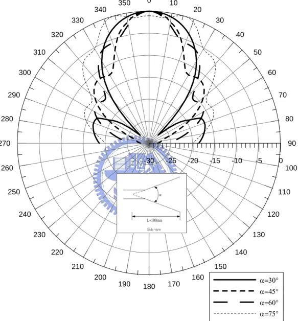
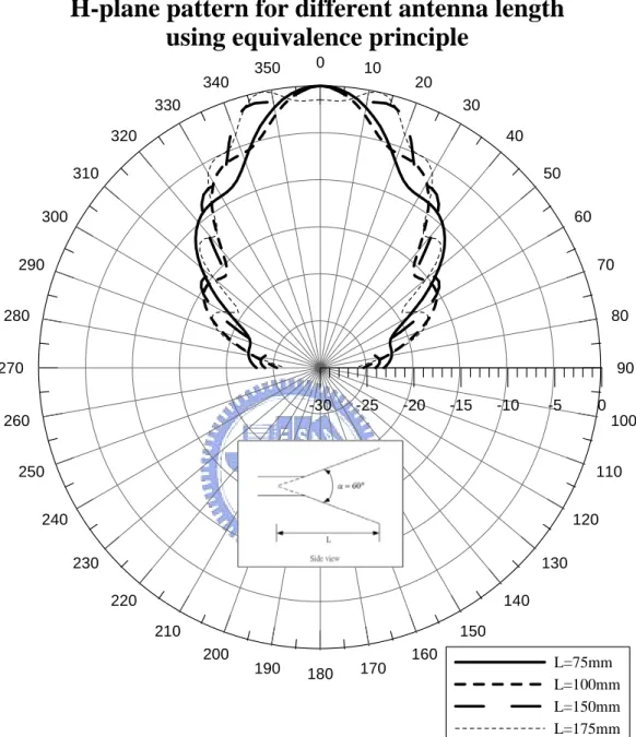
(20) To examine the behavior of the pattern as a function of flaring, the H-plane patterns for a TEM horn antenna with L=100mm and with flare angles of 30° ≤ α ≤ 60° are plotted in Fig. 2.3. As shown in the figure, the pattern becomes narrower as the flare angle increases. As the flare angle increases to 75° , the pattern becomes broad and the angle having maximum radiation intensity shifts to 15° and 345° , respectively. The maximum does not occur on axis may be concluded as the destructive interference due to the phase taper on the aperture.. Similar pattern variations occur as the length of the TEM horn is varied while the flare angle is held as constant. The H-plane patterns for TEM horn antennas with a flare angle of. α = 30° and antenna lengths of 75mm ≤ L ≤ 175mm are plotted in Fig. 2.4. As shown in the figure, the pattern initially becomes narrower but will begin to broaden and flatten as the antenna length gradually increases. Beyond a certain length, the main maximum does not even occur on axis which is demonstrated in Fig. 2.4 by the pattern with L=175mm. The reason is the same as that described in the former paragraph.. Although the analysis described above is based on a simple approximation, it still gives us some information about the tendency how the radiation beamwidth varies as the geometric parameters change. Since the ultra-wideband antennas usually cover a wide frequency range, the electrical length of the antenna is considerable. As a consequence, for the full-wave analysis, such as FEM method, there must be numerous unknows required in the field computation. The extensive memories and mathematical operations needed in the numerical simulation make it difficult to deduce the design criterion through numerous parametric studies. Therefore, the empirical formula based on simple approximation could provide us a simple, fast and low cost way to design the antenna, although, the accuracy remains to be examined in detail. 10.

(21) H-plane pattern for different flare angles using equivalence priciple 340. 350. 0. 10. 20. 330. 30. 320. 40. 310. 50. 300. 60. 290. 70. 280. 80. 270. 90 -30. -25. -20. -15. -10. -5. 0. 260. 100. 250. 110. 240. 120 230. 130 220. 140 210. 150 200. 190. 180. 170. 160. α=30° α=45° α=60° α=75°. Fig. 2.3 Computed H-plane pattern for constant length and different flare angles. 11.

(22) H-plane pattern for different antenna length using equivalence principle 350. 0. 10. 340. 20. 330. 30. 320. 40. 310. 50. 300. 60. 290. 70. 280. 80. 270. 90 -30. -25. -20. -15. -10. -5. 0. 260. 100. 250. 110. 240. 120 230. 130 220. 140 210. 150 200. 190. 180. 170. 160. L=75mm L=100mm L=150mm L=175mm. Fig. 2.4 Computed H-plane pattern for constant flare angle and different lengths. 12.

(23) Chapter 3 Design and Measurement. 3.1 Operation principle. The TEM horn antenna is one kind of traveling-wave structure, which radiates the transverse electric and magnetic (TEM) fields along the end-fire direction. They typically consist of two linear or exponential tapered metal plates that the fields in which can be considered as a TEM wave guided in a parallel two-wire transmission line. Besides, the taper transition serves as a structure to change the guided wave in the parallel-plate transmission line into a leaky wave. As a consequence, to understand the radiation characteristics of the antenna, we should first realize the wave guiding in such a taper transmission line.. The operation of the TEM horn antenna is based on the principle of wave propagation along a transmission line. In the uniform section of the parallel plate waveguide, where the spacing between the top conductor and the ground plane is smaller compared with the wavelength of operating, wave propagation is mostly confined within the region. However, when the separation between the top conductor and ground plane gradually increases, that is, the parallel-plate waveguide has some perturbations, the fields are no longer guided in the waveguide. Consequently, the energy begins to radiate in the end-fire direction and the entire structure behaves as a radiator. The discussion described above is just a very simple but 13.

(24) realistic approximation to the actual mechanism of TEM horn antennas by comparing them with a flared two-wire transmission line. In reality, the whole conditions are more complex, but this model is still a very good approximation to the actual situation. The design considerations are just based on the operation principles.. 3.2 Design considerations. Although the TEM horn antenna has been used to serve as a ground penetrating radar (GPR) system for many years, so far they have no rigorous formulation for the electromagnetic fields solutions. Various approximate analyses have been developed. To mention a few, the simplest analysis assumes a field distribution on the apertures of the horn and the open spaces along the sides of the horn. This field is assumed to be the TEM mode existed in the horn of infinite extent, where the higher order modes caused by the taper transition are ignored. Moreover, Huygen’s principle is used with this field to predict the radiating field of the horn, as described in the previous chapter. The simple approximation provides us a initial design for such a kind of antenna, although the accuracy remains to be studied in detail.. The most important subject in antenna design is the impedance matching. Such matching networks become increasingly difficult to construct for broadband operation. The reflections that occur at the aperture of the TEM horn generally degrade the performance of the antenna, and various methods have been proposed to reduce these reflections. In 1971, Wholers introduced the concept of shaping the plates of the TEM horn so as to continuously change the characteristic impedance of the equivalent transmission line over the length of the antenna. At the apex, the characteristic impedance is set to that of the feeding transmission line, and at 14.

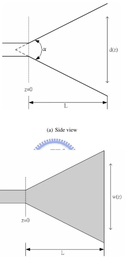
(25) the aperture it is set to the wave impedance in free space (η = 377Ω ). Although the previous method, in theoretical, could achieve the impedance match, the design is only valid for the condition of frequency independent. The dispersive for the wave impedance results in the impedance mismatch during wideband operation.. 3.3 Design procedure. The TEM horn antenna consists of a pair of triangular conductors that form some type of V-dipole structure and are characterized by L, W, d, α , which correspond to the length of antenna, the width of conductor plates, separation between two plates, and the flare angle respectively, as shown in Fig. 3.1. In the following paragraph, we will review the procedures for designing a TEM horn antenna for broadband operation.. (1) Determine the antenna length Generally, TEM horn antennas show band pass filter-like behavior with cut off frequency determined by the conductor plate length. Therefore, for a desired frequency range, the lowest frequency determines the antenna length.. (2) Arrange the taper for the conductor plates The most significant factor for the antenna design is the determination of the impedance variations from the feeding transmission line to free space. Smooth impedance variation results in small impedance discontinuities and corresponding small internal multiple reflections. The flaring, in general is linear or exponential forms. Though the later has the advantage of small reflection with the TEM wave, the linear taper has the characteristic of. 15.

(26) (a) Side view. (b) Top view. Fig. 3.1 Structure of the linearly tapered TEM horn. 16.

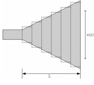
(27) easy fabrication compared with exponential type. For this reason, we have chosen the linear taper structure for the TEM horn antenna design. The degree of impedance match will depend mainly on the flare angle α .. (3) Calculate the width to height ratio of the two conductor plates A TEM horn antenna was designed to be fed through a coaxial transmission line with the characteristic impedance Z 0 = 50Ω . Once the flare angle is determined, the following approximate procedure was adopted to obtain the W/d ratio and their corresponding values.. As shown in Fig.3.2, by using the staircase approach, the structure of TEM horn antennas can be regarded as the cascade of multiple sections of parallel plate waveguides. In doing so, the characteristic impedance of each parallel-plate waveguide having width and separation distance, W(y) and d(y), respectively,. Z ( z) =. d ( y) η W ( y). (3. 28). This equation is valid under the condition that the plate width (W) is assumed to be greater than the separation distance (d). Although the conductor plate spacing becomes wider near the open end of the horn and the assumption may be violated, we still utilizing the (3.1) to obtain the first order approximation.. 17.

(28) (a) Side view. (b)Top view. Fig. 3.2 Staircase model of TEM horn. An alternative approach to determine the characteristic impedance is to replace one of the conductors by an infinite ground plane serving as an image plane. Then at any transverse cross section, the geometry for the horn is that of a microstrip transmission lines filled with free space. Therefore, the staircase horn antenna can be considered as the cascade of microstrip lines similar to that in Fig.3.2, each line has its own characteristic impedance. The aspect ratio W/d that gives the desired characteristic impedance is determined by the formula [1], which is given below:. Z0 =. 120π 2W / d + 1.393 + 0.667 ln( 2W / d + 1.444). for W / d ≥ 1. (3. 29). Because of symmetry, the characteristic impedance at each cross section is half of the original one without image plane. For example, the W/d ratio at the feed point for this new equivalent structure should be chosen to have 25Ω characteristic impedance rather than 50Ω .. Both the previous two procedures could provide us the similar, however, not so accurate 18.

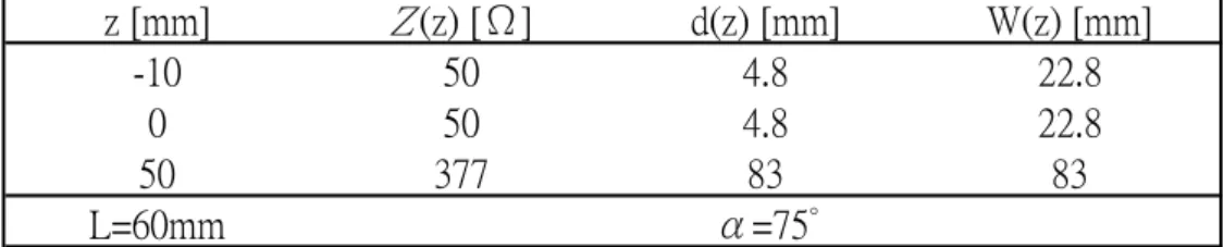
(29) design parameters. Since both of these two models are approximations, further adjustment for the antenna size is needed. However, the size for fabrication remains to be calculated by means of full wave analysis, such as FEM (finite element method) or FDTD, which will be demonstrated in the next section.. 3.4 Full wave simulation of TEM horn antennas. Since structural parameters obtained from the procedures that described previously are first order approximation, it is necessary to adjust these initial designs. In this research work, the Ansoft HFSS simulation tool is employed by full wave simulation to refine design parameters obtained by the initial ones. When modeling fully 3-D antennas using HFSS, there are several factors that should be taken into account to have a good management in memory usage. Because the computation is performed within a finite volume, the perfect matching layer (PML) boundary condition is used to truncate the infinite space into a finite one. Such a kind of boundary condition must be set at least quarter wavelength away from the antenna with respect to the lowest frequency of operation. To reduce the large amount of memory required for computation, the symmetry in field distribution of the antenna allows us to simulate part of the original structure by imposing suitable boundary condition. In detail speaking, the plane y=0 is set to be a perfect H plane with its port impedance multiplied by 2 while that x=0 is designated as a perfect E plane with its port impedance divided by 2. The antenna is fed through lump port with 50Ω port impedance containing only the TEM mode wave. Finally, the results of the simulation are shown in Table 3.1.. 19.

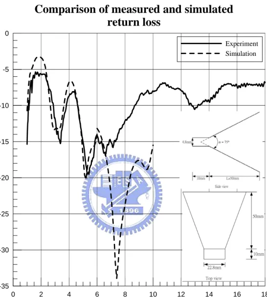
(30) z [mm] -10 0 50 L=60mm. Z (z) [Ω]. d(z) [mm] 4.8 4.8 83 α=75°. 50 50 377. W(z) [mm] 22.8 22.8 83. Table 3.1 Antenna dimensions. 3.5 Fabrication and measurement. The antenna is manufactured based on the results from simulation as depicted in Table 3.1. The material for the conducting plates is copper with 0.20 mm thickness to reduce the weight of the antenna. The conductivity of this copper plate is equal to 5.813 × 10 7 (. 1 ). ohm • m. For supporting and fixing the plates, polystyrene with relative permittivity very close to unity is used to minimize the effects on the antenna. The total antenna length is 60 mm and the dimension of the aperture is 83× 83 mm. The antenna is fed through a coaxial cable with the SMA connector. The parallel-plate waveguide having the dimension of 76 × 16 mm and 10 mm length is as a transition structure for the wave from the coaxial mode to the parallel-plate one.. The return loss is measured by the HP 8722D network analyzer. Fig. 3.2 shows the comparison of calculated and measured return loss of this antenna in the frequency range from 1GHz to 18GHz. As depicted in the figure, the calculated and measured agree very well for frequency lower than about 6.5 GHz. But the electromagnetic energies above that frequency obviously were not fed into the antenna. However, from the measured data shown in this figure, for the frequency beyond 6.5 GHz, this antenna experiences a strong reflection at the input port. We may conjecture that during modeling we have assumed the antenna 20.

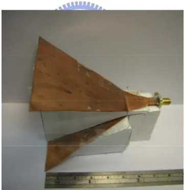
(31) guided only the TEM waves by assigning the lump port at the feed point. However, in reality the antenna is fed by coaxial cable with SMA connector. Due to unbalance nature of a coaxial cable, the direct connection introduces unbalance currents on the plates of the TEM horn that is a balance antenna.. The conductor plate spacing at the feed point should be comparable to that between the inner and outer conductor of the attached coaxial cable. This limitation is due to the fact that otherwise a large geometrical discontinuity is introduced at the antenna’s feed point and the TEM horn structure cannot any more be approximated as coaxial cable extension. Therefore, the tapered transition of the top conductor and ground plate is introduced between the parallel plate and the V-shape section. Such a structure has the advantage of being mechanically suitable for connecting to TEM horns. The dimension of the final design is re-built in Table 3.2. The fabricated antenna based on the table is shown in Fig. 3.3.. z [mm]. Z(z) [Ω]. d(z) [mm]. W(z) [mm]. -20. 50. 1.6. 7.6. -10 0 50. 50 50 377. 1.6 4.8 83. 7.6 22.8 83. L=50mm. α=75°. Table 3.2 Antenna dimensions added with taper transition. 21.

(32) Comparison of measured and simulated return loss 0. Experiment Simulation -5. -10. -15. -20. -25. -30. -35 0. 2. 4. 6. 8. 10. 12. 14. 16. 18. Fig. 3.3 Distribution of return loss against frequency for both measured and calculated results of the antenna based on Table 3.1. 22.

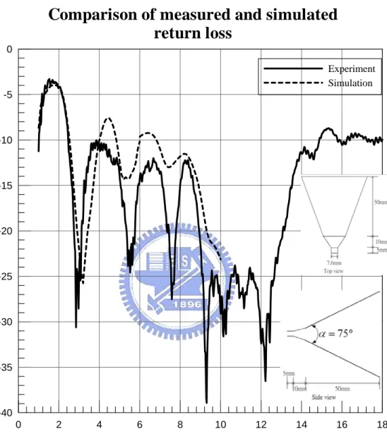
(33) The comparison of simulated and measured return loss of this new antenna in the frequency band from 1GHz to 18GHz is shown in Fig. 3.4. The measured return loss of this new antenna shows a good agreement with numerical simulation by using Ansoft HFSS over a wide frequency range. The TEM horn has an operational bandwidth from 2.4 GHz to 15 GHz for return loss larger than 10 dB. The aspect ratio for the operation frequency is 6.25. Thus, the antenna has a 12.6 GHz or 6.25:1 operational bandwidth. The bandwidth shows that it indeed is an ultra-wideband antenna. By means of this experiment, it also validate the design procedure employed in this thesis.. Fig. 3.4 The fabricated TEM horn antenna. 23.

(34) Comparison of measured and simulated return loss 0. Experiment Simulation -5. -10. -15. -20. -25. -30. -35. -40 0. 2. 4. 6. 8. 10. 12. 14. 16. 18. Fig. 3.5 Distribution of return loss against frequency for both measured and calculated results of the antenna added with taper transition. 24.

(35) The far-field radiation patterns of this antenna were performed in anechoic chamber. Figs. 3.5 to 3.7 show the calculated and measured radiation pattern on the H plane at 5, 7, and 9 GHz respectively. The calculated pattern using equivalence principle is in reasonable agreement with the experiment result within a certain range of elevation angle except the one at 9 GHz. The difference in magnitude between calculated and experimented data for θ ≥ 20° becomes obvious, it is because that the equivalent principle is valid only for the forward radiation. Therefore, even if the bandwidth of this antenna could meet our design specification from 2 GHz to 11 GHz, its radiation characteristic remains to be improved in practical applications. In the next chapter, we will investigate the variation on the radiation pattern of the TEM horn antenna by changing the structural parameters, such as the flare angle, transition length and etc. Having these information in mind, we could establish a engineering design criterion for such a type of antenna.. 25.

(36) H-plane pattern at 5 GHz 340. 350. 0. 10. 20. 330. 30. 320. 40. 310. 50. 300. 60. 290. 70. 280. 80. 270. 90 -35. -30. -25. -20. -15. -10. -5. 0. 260. 100. 250. 110. 240. 120. Experiment Approximation. 230. 130. 220. 140 210. 150 200. 190. 180. 170. 160. Fig. 3.6 The measured and calculated H-plane radiation pattern of the TEM horn at 5 GHZ. 26.

(37) H-plane pattern at 7GHz 340. 350. 0. 10. 20. 330. 30. 320. 40. 310. 50. 300. 60. 290. 70. 280. 80. 270. 90 -30. -25. -20. -15. -10. -5. 0. 260. 100. 250. 110. 240. 120 Approximation Experiment. 230. 130. 220. 140 210. 150 200. 190. 180. 170. 160. Fig. 3.7 The measured and calculated H-plane radiation pattern of the TEM horn at 7 GHZ. 27.

(38) H-plane pattern at 9GHz 340. 350. 0. 10. 20. 330. 30. 320. 40. 310. 50. 300. 60. 290. 70. 280. 80. 270. 90 -40 -35 -30 -25 -20 -15 -10. -5. 0. 260. 100. 250. 110. 240. 120 230. 130. Approximation Experiment. 220 210. 140 150. 200. 190. 180. 170. 160. Fig. 3.8 The measured and calculated H-plane radiation pattern of the TEM horn at 9 GHZ. 28.

(39) Chapter 4 Variation of Parameters. 4.1 Motivation. In the previous chapter, we have designed a TEM horn antenna that has ultra-wideband characteristic. In this chapter, we want to develop design criterion for fabricating TEM horn antennas meeting the specification. Because the computation by FEM method should be performed within a finite volume, air box and perfect matching layer boundary condition are required to truncate the infinite volume into a finite one. The distance between boundaries of the air box and antenna should be at least quarter wavelength corresponding to the operational frequency. However, since the ratio of maximum to minimum frequency is usually large for ultra-wideband antennas, the dimension of air box set for the lowest frequency will be too large compared with its highest frequency. Then the computation time will be excessively long for full band simulation. Although we can divide the entire frequency band into several sub-bands and utilize the bisection characteristic for the symmetrical feature of this antenna to reduce the computation time as being done in the previous chapter, it is not efficient for characterizing the radiation characteristic of this antenna by full-wave simulation, since there are too many structural parameters should be changed to see this influence. Thus, in this chapter, we will concentrate ourselves on the studies of radiation beam pattern based on the empirical model of the aperture field and invoking the equivalence principle. Since the 29.

(40) empirical formula does not contain the effect of several parameters, such as the transition length, flare angle and etc. on the aperture field distribution, this may be the main problem resulting the errors between the measured and calculation results for a few extreme cases, which will be become clear later on.. 4.2 Design considerations. Since full- wave simulation is no longer utilized to predict the behavior of antennas, we should make certain that the antenna could maintain its radiation for a ultra-wideband. At the feed point, we use the same feeding structure shown in chapter 3 to guarantee the matching at the input end. On the other hand, since we can regard the cross section of the aperture as a parallel plate waveguide, then the characteristic impedance for parallel waveguide can be written as follows.. Z=. d η w. (4. 30). where d and W are the separation distance between two metal plates and the width of metal plate, respectively.. Since the wave impedanceη of air is roughly equal to 377Ω , the. d ratio is set to be W. unity that the aperture of an antenna is matched to free space. Therefore, with the given distance between two plates at the feed point, the separation at the aperture can be determined from the desired antenna length and flare angle. The corresponding plate widths are then equal to their separation. In the next step, we study the effect of the antenna length and flare angle on the antenna performance. The Matlab program based on the equivalence principle 30.

(41) described in chapter 2 will also be developed to obtain the design reference before implementing the antenna.. 4.3 Effect of antenna length on the radiation characteristics. The first three cases demonstrate the variation of H-plane radiation pattern and operational bandwidth for various antenna lengths and constant flare angle. In general, we observed that the measured H-plane pattern agrees with computation by equivalence principle under the condition of smaller flare angles. Therefore, firstly we fixed the flare angle α to. 30° and varied the antenna length from 50mm to 100mm with 25mm increment. The measured return loss for these three antennas is shown in Fig. 4.1. Evidently, the antennas fabricated based on the design procedure described in the previous section exhibit ultra-wideband characteristic. For example, the antenna with 50mm length has the widest bandwidth more than 18GHz, while the one with 100mm length can extend to the lower frequency.. The comparison of measured and calculated H-plane patterns at 7GHz for these three cases are shown from Fig. 4.2 to 4.4. In these figures, one could observe that the 3dB beamwidth decreases as the increase in the antenna length. Besides, the back lobes for the three cases are -7dB, -13dB and -18dB, respectively. The back lobe level is considerable for small size antennas. This is because, for a given flare angle, the impedance mismatch is obvious for the case of small antenna length, thus, the incident power will directly reflected and produce a strong radiation in the backward direction. On the contrary, the antenna for 100mm long has lower back lobe, below -15dB. In a word, though the short antenna has the wide bandwidth, the long antenna has small back lobe level. These figures also verified again that the measured radiation patterns are in considerable agreement with those calculated 31.

(42) according to equivalence principle. Although the approximation method is hard to predict the side lobe level, however, the side low levels for all cases in our experiments are lower than -15 dB. Thus, it affects the radiation characteristic inconsiderably. Therefore, the program developed in this thesis is able to predict radiation pattern prior to fabricate the antenna, therefore, it further reduces the time consuming for cut-and-try.. 4.4 Effect of flare angle on the radiation characteristics. In chapter 3, we have designed a TEM horn antenna with 75° flare angle and 50mm length. As mentioned in that section, the measured return loss consisted very well with computation based on Ansoft HFSS simulation tool. However, the approximated radiation patterns using equivalence principle coincide with measured ones only within a small range of elevation angle ( θ ≤ 20 ). The disagreement becomes apparent especially for the high frequency range of operation. However, for all the three examples with a 30° flare angle in the preceding section, the equivalence principle could well predict the radiation pattern in both amplitude and shape as shown in Fig.3.2 ~ Fig.3.4. From these figures we may conjecture that the factor determining the accuracy of approximation is the flare angle. Therefore, it is needed to explore the accuracy of this approximation for engineering design in practice.. On the other hand, it is also necessary to examine the variation of radiation characteristics for various flare angles while the antenna length is fixed. In this section, several experiments were carried out to demonstrate how the radiation behavior varies with different flare angles. Since the antenna with a 100mm in length in the preceding section exhibits low back lobe, the antenna length was fixed at 100mm and the flare angle was 32.

(43) increased progressively from 30° to 60° with 15° increment to measure its radiation pattern.. The measured H-plane pattern at 7 GHz for three different flare angles are respectively shown in Fig.4.4, 4.5, and 4.6. It could be seen that calculated radiation patterns agree with that by measurement for the two cases of α = 30° and 45° . For all frequency within the bandwidth, we will obtain the same good agreement. But for the case with a flare angle of 60° , the measured pattern is much wider than the computed one. The inconsistence between measurement and calculation will become obvious for higher frequency range, as shown in Fig.3.7. The reason for this deviation could be inferred as follows. In chapter 2 we assumed the field distribution on the aperture to according to equation (2.19)-(2.20) and zero outside the aperture. Based on the experiment studies, we observed that the empirical formula is valid for the flare angle small than 45° .. As the flare angle increases, the separation changes. accordingly. Under this condition, the approximated aperture field distribution is no longer valid. Moreover, the edge diffraction effect might be obvious in the situation such that the assumption of zero fields outside aperture remains to be modified. This diffraction has significant effect on its radiation as shown in Fig. 4.6.. In generally speaking, the H-plane 3dB beamwidth decreases as the flare angle increases. We have plotted the half-power beamwidth as a function of flare angle at 7GHz, as shown in Fig.4.7. Similar figures can also be obtained for arbitrary antenna lengths and frequencies. An improvement of this figure can be made by representing the antenna length in its electrical length and then we can obtain this new figure as shown in Fig. 4.8. However, for a given length, the antenna exhibits a monotonic decrease in 3dB beamwidth up to a certain flare angle. Beyond that point an increase in beamwidth is observed. It can be accounted for the broadening in the main beam as shown in Fig. 4.6.. 33.

(44) Return loss for various antenna length with α=30° 0. L=50mm L=75mm L=100mm. -5. -10. S11(dB). -15. -20. -25. -30. -35. -40. -45. 0. 2. 4. 6. 8. 10. 12. 14. 16. 18. Frequency(GHz). Fig. 4.1 Measured return loss for antennas with fixed flare angle α = 40° and three different antenna lengths. 34.

(45) H-plane pattern at 7GHz with α=30°, L=50mm 340. 350. 0. 10. 20. 330. 30. 320. 40. 310. 50. 300. 60. 290. 70. 280. 80. 270. 90 -30. -25. -20. -15. -10. -5. 0. 260. 100. 250. 110. 240. 120 230. 130. Experiment Approximation. 220 210. 140 150. 200. 190. 180. 170. 160. Fig. 4.2 Measured and calculated H-plane patterns with. α = 30° and L=50mm at 7GHz. 35.

(46) H-plane pattern at 7GHz with α=30°, L=75mm 340. 350. 0. 10. 20. 330. 30. 320. 40. 310. 50. 300. 60. 290. 70. 280. 80. 270. 90 -30. -25. -20. -15. -10. -5. 0. 260. 100. 250. 110. 240. 120 230. 130. Experiment Approximation 220. 140 210. 150 200. 190. 180. 170. 160. Fig. 4.3 Measured and calculated H-plane patterns with. α = 30° and L=75mm at 7GHz. 36.




(50) 3-dB beamwidth as a function of flare angle 90 85 80 75 70 65. 3-dB beamwidth. 60 55 50 45 40 35 30 25 20. 5GHz 7GHz 9GHz. 15 10 5 0 15. 20. 25. 30. 35. 40. 45. Flare angle(α). Fig. 4.7 3dB beamwidth in H-plane of TEM horn antennas as a function of flare angle with a given antenna length L=100mm. 40.

(51) 3-dB beamwidth as a function of flare angle for different lengths 50. 45. 3-dB beamwidth (degree). 40. 35. 30. 25. 20. 15. 10. r0=5λ r0=10λ. 5. r0=20λ 0 10. 15. 20. 25. 30. 35. Flare angle α (degree). 40. 45. 50. Fig. 4.8 3dB beamwidth in H-plane of TEM horn antennas as a function of flare angle for different lengths. 41.

(52) Chapter 5 Conclusion. Due to the feature of easy fabrication for a TEM horn antenna having linear taper transition, in this thesis, we have proposed a design procedure based on the simple transmission line model and Ansoft HFSS full-wave simulation tool both. By mutually examining between the two methods, a TEM horn antenna is able to operate from 2.4 GHz to 15GHz, for return loss less than -10dB. In this work, the measurements are in good agreement with computations. It is also verified that the proposed design procedure is suitable for antenna design in ultra-wideband applications, such as GPR and EMC measurement systems.. We intend to improve the radiation characteristic of proposed horn while reducing the time consumption in the simulation. In a systematic manner, several examples have been demonstrated to investigate properties of structural parameters, the antenna length (L) and flare angle (α ) . It can be concluded that the antenna length (L) determines the bandwidth and lowest frequency. Besides, the back lobe level is lower for large antenna length. As for flare angle (α ) , in general, the H-plane pattern has narrow beamwidth for small flare angle.. The field equivalence principle has been employed to analyze several TEM horn antennas. The computed results are in good agreement with experiments for flare angle of antennas small than about 45° . These results show that the equivalence principle method is 42.

(53) useful for evaluating the radiation pattern of TEM horn antennas. Therefore, we can plot the H-plane half-power beamwidth as a function of flare angle for different lengths. Such a kind of figure can be served as a design criterion to have a antenna, which is able to meet the prescribed specification.. 43.

(54) Reference [1] David Pozar, “Microwave Engineering”, 2nd Edition, John Wiley & Sons, N. Y., 1998 [2] Constantine A. Balanis , “Antenna Theory”, 2nd Edition, John Wiley & Sons, N. Y., 1997 [3] Kanda M, “Transients in a resistively loaded linear antenna compared with those in a conical antenna and a TEM horn”, Antennas and Propagation, IEEE Transactions on [legacy, pre - 1988] , Volume: 28 , Issue: 1 , Jan 1980 , Pages:132 - 136 [4] Hyoungjin Cho and Sangseol Lee,” Design of an exponentially-tapered TEM horn antenna for the wide broadband communication”, Microwave and Optical Technology Letters, Volume 40, Issue 6, Date: 20 March 2004, Pages: 531-534 [5] Mayes J.R. and Carey W.J. “The generation of high electric field strength RF energy using marx generators”, Conference Record for the 25th International Power Modulator Symposium, 2002 [6] Ahmet Serdar Turk, “Ultra-wideband TEM horn design for ground penetrating impulse radar systems”, Microwave and Optical Technology Letters , Volume 41, Issue 5, Date: 5 June 2004, Pages: 333-336 [7] Ivor L Morrow, “TEM horn optimized for transient radiation”, Microwave and Optical Technology Letters, Volume 30, Issue 3, Date: 5 August 2001, Pages: 161-164 [8] Lewin L, Nakhkash M and Yi Huang, ”Directive wideband TEM horn antenna for precise free-space measurements”, Precision Electromagnetic Measurements, 2002. Conference Digest 2002 Conference on, 16-21 June 2002, Pages: 140 – 141 [9] Lai A.K.Y, Sinopoli A.L and Burnside W.D, “A novel antenna for ultra-wide-band applications”, Antennas and Propagation, IEEE Transactions on , Volume: 40 , Issue: 7 , July 1992 Pages:755 - 760 [10] Li-Chung, Chang T and Burnside W.D, “An ultrawide-bandwidth tapered resistive TEM 44.

(55) horn antenna”, Antennas and Propagation, IEEE Transactions on , Volume: 48 , Issue: 12 , Dec. 2000 Pages:1848 - 1857 [11] Nguyen C, Jeong-Soo Lee and Joong-Suk Park, “Ultra-wideband microstrip quasi-horn antenna”, Electronics Letters , Volume: 37 , Issue: 12 , 7 Jun 2001, Pages:731 - 732 [12] Maloney J.G. and Smith G..S, “On the characteristic impedance of TEM horn antennas”, Antennas and Propagation Society International Symposium, 1995. AP-S. Digest , Volume: 1 , 18-23 June 1995, Pages:182 - 185 vol.1 [13] Shlager K.L, Smith G.S and Maloney J.G, “Accurate analysis of TEM horn antennas for pulse radiation”, Electromagnetic Compatibility, IEEE Transactions on , Volume: 38 , Issue: 3 , Aug. 1996, Pages:414 – 423 [14] Lee R.T and Smith G.S, “A design study for the basic TEM horn antenna”, Antennas and Propagation Magazine, IEEE , Volume: 46 , Issue: 1 , Feb. 2004 Pages:86 - 92 [15] Yarovoy A.G, Schukin A.D, Kaploun I.V and Ligthart L.P,”The dielectric wedge antenna”, Antennas and Propagation, IEEE Transactions on , Volume: 50 , Issue: 10 , Oct. 2002 Pages:1460 – 1472 [16] Jing Li, Zhu X.Y, Wang M.X and Lang Jen, “A new design of TEM horn antennas for pulse radiation”, Microwave Conference Proceedings, 1997. APMC '97., 1997 Asia-Pacific , 2-5 Dec. 1997, Pages:629 - 631 vol.2 [17] Kyung-Ho Chung, Sung-Ho Pyun, Chung S.-Y and Jae-Hoon Choi, “Design of a wideband TEM horn antenna”, Antennas and Propagation Society International Symposium, 2003. IEEE , Volume: 1 , 22-27 June 2003, Pages:229 - 232 vol.1. 45.

(56)