針對迴旋編碼的維特比解碼機中倖存路徑器之改良

全文

(1)國立交通大學電信工程學系碩士論文針對迴旋編碼的維特比解碼機中倖存路徑記錄器之改良 “Improved Survivor Memory Unit (SMU) Designs of Viterbi Decoder for Convolutional Coding”. 研究生：林冠亨 Lin, Guan-Henry 指導教授：李程輝博士 Dr. Lee, Tsern-Huei 中. 華. 民. 國. 九十四. 年. 六. 月.

(2) Improved Survivor Memory Unit (SMU) Design of Viterbi Decoder for Convolutional Coding By Lin, Guan-Henry. Thesis submitted to the Faculty of the National Chiao-Tung University in fulfillment of requirements for the degree of. Master of Science In Communication Engineering. Dr. Lee, Tsern-Huei. June, 2005 Hsinchu, Taiwan. Keywords: Viterbi decoder, Survivor Memory Unit (SMU), REA Traceback, Memory Management. Copyright 2005© Lin Guan-Henry.

(3) 針對迴旋編碼的維特比解碼機中倖存路徑器之改良學生: 林冠亨. 指導教授: 李程輝博士. 國立交通大學電信研究所. 摘要. 在本論文中，我提出三種新的倖存路徑記錄器之設計來分別改良三種傳統倖存記錄器實現方法的缺失。對路徑回溯法(Traceback Management)而言，它原本就具備低功率消耗及較小的電路面積，但最為詬病的是其過程需要長時間的延遲 (Decoding latency)。針對路徑回溯法，我提出跳階路徑回溯法(Stage-Hopping TBM).改良後的解碼效率隨著強制長度(Constraint Legnth)的增加可以逼近暫存器交換法(Register Exchange)的解碼效率。除此之外，改良後的跳階回溯法所用來記錄路徑的記憶體量只需原來路徑回溯法的 45%。因此跳接路徑回溯法可同時改善維特比解碼機的解碼效率以及硬體的複雜度。對於暫存器交換法而言，儘管它有最短的解碼延遲，它的功率消耗以及電路面積卻是三種傳統方法中需要最大的，原因在於暫存交換法所需要極大量的暫存器與多工器(Multiplexer)將倖存路徑儲存於正確的位置中。因此，我提出了簡易暫存器交換法(Facilitated REA)，主要目的就是要減少實現暫存器交換法所需的硬體，而改良後的方法可以發現，原本多個多工器可以被單一個取代而不影響解碼的效果。對於混合法(Hybrid Method)而言，其原本被提出的目的就是要藉由結合路徑回溯法與暫存器交換法的優點來中和兩者的缺點，因此可以明顯的發現，前述提出的改良方法皆可同時應用在混合法中，以求進一步的改善實現混合法所需的硬體複雜度。在所提出的三個新方法中，用來查詢出路徑對應輸入信號為何的解碼單位 (Decision Unit)都是不被需要的，因此些許的硬體和解碼延遲都可以再被減少。總結而言，藉由 C 語言的模擬可以發現，新提出的倖存路徑記錄器設計並不會因為改良硬體需求與解碼效率就犧牲解碼能力。藉由圖形表示法(Graphic representation)，三種改良方法的解碼效率和硬體需求都可以被詳細檢視與比較，藉此可看出每種新提出的改良設計所能獲得的好處。. ii.

(4) Improved Survivor Memory Unit (SMU) Design of Viterbi Decoder for Convolutional Coding. Lin, Guan-Henry Dr. Lee, Tsern-Huei Department of Communication Engineering. (Abstract) In the thesis, three new approaches are proposed to improve the drawbacks of three corresponding methods that are used conventionally in the realization of survivor memory unit (SMU) in Viterbi Algorithm (VA) as convolution decoders. For trace-back management (TBM) method, it has owned the virtues as low power consumption and small circuit area, but suffers long decoding latency. Corresponding to TBM, Stage-Hopping TBM (SH-TBM) is developed. The decoding efficiency can be raised approaching to the performance of register exchange algorithm (REA) as constraint length increases. On the other hand, length of the required memory could be reduced down to about 45% of the length originally required in TBM at most. REA obtains shortest decoding latency, however, with large power consumption and circuit area caused by the required numbers of registers and multiplexers. To ameliorate the disadvantage, Facilitated REA (FREA) is proposed with a concept that multiple of multiplexers can be replaced by a single one without affecting the decoding performance. As for Hybrid method, it is originally designed to balance the trade-off between decoding efficiency and the required quantity of hardware by combining TBM and REA. Therefore, Improved Hybrid method (IHY) naturally inherits the technique used in FREA and SH-TBM. As expected, fewer multiplexers, in some cases only one column of multiplexers, will be needed and traceback operation could be realized faster. Of all three newly proposed methods, decoding unit (DU) is eliminated. Hence, a slight more increase in speed and decrease in hardware could be acquired. In summary, the experimental result simulated by C program shows that proposed methods do not deteriorate the decoding performance anyhow. By graphical methods, analyses and comparisons are made to demonstrate the improvements in hardware reduction and the acceleration in decoding efficiency. iii.

(5) Acknowledgements First, I have to express my gratitude to Prof. Lee who has offered me a free space to complete my research independently and tolerated my decisions in everything. Also, I am grateful to be given the chance by Prof. Lee to present my idea in Shang-Hai last October. These experiences will definitely serve as stepping stones to my future researches and advanced studies. I can never get into the communications field so deep, especially in coding theory and its applications, without mentioning of Prof. Chang, Wen-Whei and Dr. Hsu, Heng-Iang. I can not thank these three guides enough. In addition, I am so pleased to be in the family of NTL laboratory. With companion of members in the lab, I enjoy every minute of laughter and bitterness. I will take the lessons I learn from each of them along the way in my life. Last but not least, I have to and more than willing to dedicate my strongest gratitude to my family, my Father, Mother and my little sister. With their support, I can conquer everything in the world. In case, thanks to those who has ever helped me but I accidentally missed. I will expiate by listing you in the acknowledgement of my future papers.. iv.

(6) Contents 1 Introduction………………………………………………………………………….1 1.1 Organization of the thesis…………………………………………………….2 2 Viterbi Algorithm and SMU implementation technique.............................................3 2.1 Overview and introduction…………………………………………………...3 2.2 Convolutional codes………………………………………………………….3 2.3 Viterbi decoder……………………………………………………………….6 2.4 Survivor memory unit (SMU)………………………………………………..9 2.4.1 Traceback management (TBM)…………………………………….9 2.4.2 Register exchange algorithm (REA)……………………………...12 2.4.3 The Hybrid method……………………………………………….13 2.5 Summary of the chapter…………………………………………………….15 3 Three improved SMU designs……………………………………………………...16 3.1 Overview……………………………………………………………………16 3.2 The observation……………………………………………………………..16 3.3 Stage-Hopping TBM (SH-TBM)…………………………………………...18 3.4 Facilitated REA (FREA)……………………………………………………21 3.5 Improved hybrid method (IHY)…………………………………………….23 3.6 Summary of the Chapter……………………………………………………25 4 Experimental results and analyses………………………………………………….26 4.1 Decoding performance……………………………………………………...26 4.2 Decoding efficiency and hardware reduction……………………………….27 4.2.1 TBM vs. Stage-Hopping TBM……………………………………27 4.2.2 REA vs. Facilitated REA………………………………………….31 4.2.3 Hybrid method vs. improved hybrid method……………………..33 4.3 Power dissipation and summary of the chapter……………………………..35 5 Conclusion………………………………………………………………………….36 5.1 Conclusion…………………………………………………………………..36 5.2 Future work…………………………………………………………………37 Bibliography……………………………………………………………………….…38 Appendix A. VLSI program documentation…………………………………………39. v.

(7) List of Tables. Table I: Performance of Viterbi decoder with different memory management techniques of SMU…………………………………………………………………26 Table II: Analysis of TBM…………………………………………………………28 Table III: Analysis of SH-TBM……………………………………………………30 Table VI: Analysis between REA and FREA………………………………………32 Table V: Analysis between Hybrid method and Improved Hybrid method………..34. vi.

(8) List of Figures. Figure 2.1: Block diagram of rate 1/2-Convolutioanl encoder………………………4 Figure 2.2: Block diagram of rate 2/3-Convolutional encoder………………………4 Figure 2.3: Example of recursive convolutional (RSC) encoder…………………….5 Figure 2.4: Trellis diagram for rate 1/2-convolutional code…………………………6 Figure 2.5: Illustration of ACS recursion for M=2…………………………………..8 Figure 2.6: The generation of common tail………………………………………….9 Figure 2.7: The entire Viterbi Decoder block diagram………………………………9 Figure 2.8: Example of TBA………………………………………………………...10 Figure 2.9: Different TB memory contents (a) previous states (b) decision values…11 Figure 2.10: Hardware Architecture of REA………………………………………...13 Figure 2.11: Example of Hybrid method…………………………………………….14 Figure 3.1: Phenomena of the same output for a certain state……………………….17 Figure 3.2: Three-step Trellis for a (2,1,3) code……………………………………..18 Figure 3.3: The procedure of Stage-Hopping TBM…………………………………20 Figure 3.4: Elementary component structure of the FREA method…………………22 Figure 3.5: Equivalent function of SH-TBM and the elementary component of FREA……………………………………22 Figure 3.6: The hardware structure of FREA………………………………………..24 Figure 3.7: Example of the mixed traceback and decision operations………………25 Figure 4.1: Graphic representation of a conventional TBM…………………………27 Figure 4.2: Required memory size of decision value method and SH-TBM………..28 Figure 4.3: TBM decoder design and SH-TBM decoder design…………………….29 Figure 4.4: Graphic representation of SH-TBM……………………………………..29 Figure 4.5: Decoding Efficiency of TBM and SH-TBM…………………………….30 Figure 4.6: Memory reduction ratios………………………………………………...31 Figure 4.7: Graphic representations of REA and FREA…………………………….31 Figure 4.8: Different register allocations of REA and FREA……………………….32 Figure 4.9: Simulation results of elementary component of FREA…………………33 Figure 4.10: Graphic representation of Hybrid method…….……………………….33 Figure 4.11: Graphic representation of IHY…………………………………………34. vii.

(9) Chapter 1. 1/40. Chapter 1. Introduction Convolutional coding [1] is widely employed in digital communication systems and signal processing to achieve low-error-rate data transmission. For example, IS-95, a wireless digital cellular standard for CDMA (code division multiple access), employs convolution coding, so does DVB-T system and many systems else. It offers an alternative to block codes for protected transmission over a noisy channel. The Viterbi Algorithm (VA) [2], proposed in 1967 by Viterbi, is a representative decoding procedure for convolutional codes. When erroneous data are received, the closest codeword is selected using the maximum likelihood decoding (MLD). In the hardware implementation, it is composed of three components: Add-Compare-Select (ACS) unit, Survivor Memory Unit (SMU) and Decision Unit (DU). Although VA has been applied for decades, researchers still attempt to improve it in two aspects. Efficiency is one of the issues. Many researchers had targeted on the ACS procedure when it comes to increase in decoding speed [3]. Most of them modified the ACS process by adding more parallel hardware to decode signal sequences at the same time. With this idea, more calculations could be done within a certain period of time. Thus, a task with the same burden of complexity could be realized sooner. By introducing parallel ACS modules decoding efficiency can be raised, however, more hardware/area is required. Therefore, one conclusion has been commonly drawn out of these researches is that the area/rate trade-off is linear [4]. The other issue is focused on hardware reduction in the Survivor Memory Unit. There are three common implementation methods of SMU: traceback management (TBM), register exchange algorithm (REA) and Hybrid method [5,6,7,8]. For the proper function of VA, conventionally, memory length in TBM or the number of registers and multiplexers in REA has to be equal to the length of entire sequence. Fortunately, through theoretical demonstration and simulations by many researchers [9], they find that a value of 4 or 5 times the code constraint length is sufficient for negligible degradation from optimal performance of the decoder. With sufficient length of sequence, common tails will appear so that the memory size in TBM and the number of registers and multiplexers in REA could be reduced to a practical extent. Even with the existing progress made in these two issues, the first question mounting in my mind is that attempts to increase decoding efficiency by modifying ACS unit will bring about the need of extra hardware. Then, why not turn to modify procedure of other components in VA? On the other hand, is the further reduction of 1.

(10) Chapter 1. 2/40. hardware used in SMU possible? Bearing these two questions in mind, we find the key lies in the SMU. It is based on the observation that the latency in TBM still leaves some room for improvement and further hardware reduction in TBM and especially in REA is eagerly demanded. Thus, we determine to search for new approaches to realize SMU with faster decoding speed and less hardware requirements. Thus, the theme of the research is set on the improved survivor memory unit design of Viterbi decoders. We start by observing trellis diagrams of some commonly used convolutional coders in the digital communication systems. Eventually, an innate characteristic is found to be applied on the three conventional methods and evolve into three newly proposed SMU designs so as to reach the expected improvements. 1.1 Organization of the thesis The organization of this thesis can be described as follows: The background on the operation of convolutional encoders and Viterbi decoders will be provided in the Chapter 2 and emphasize on descriptions of three conventional SMU implementation methods – TBM, REA and the Hybrid method. In the Chapter 3, the main concept extracted from our observations will be introduced and also how it is then incorporated into the three conventional methods separately for improvements. Experimental results in decoding performance and graphical analyses of hardware requirements will be discussed later in the Chapter 4 along with detailed comparisons. At last, Chapter 5 will conclude the thesis and indicate the future works.. 2.

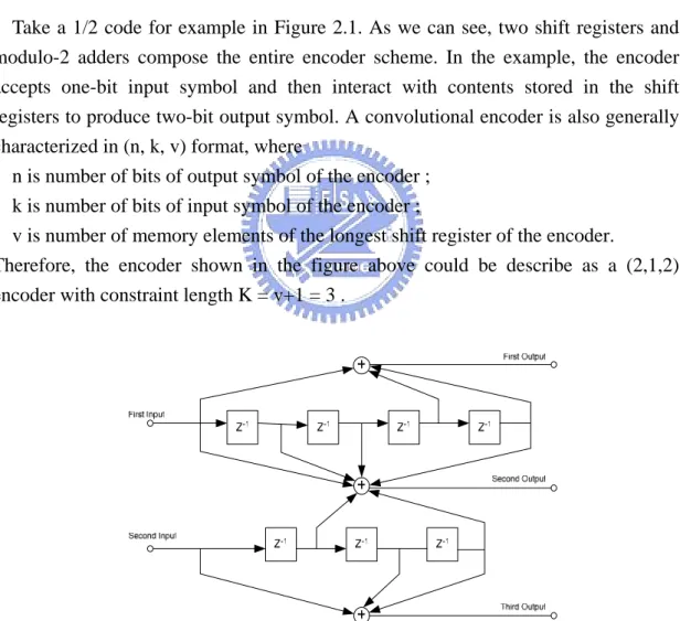
(11) Chapter 2. 3/40. Chapter 2. Viterbi Decoding Algorithm and SMU Implementation Techniques 2.1 Overview and Introduction In this chapter, necessary background on the research will be provided. First, convolutional codes are discussed and then we will explain the Viterbi decoding algorithm and its decoder design. In the design, survivor memory unit (SMU) is focused and three conventional methods used in the SMU will be introduced. 2.2 Convolutional codes Due to the imperfectness of channels, errors would often occur during transmission. Therefore, some measurements must be taken to combat the disturbance and to raise the reliability of communication systems. One practical option to deal with the problem is called error-control coding or channel coding. The channel encoder in the transmitter accepts message bits and adds redundancy according to a prescribed rule, thereby producing encoded data at a higher data rate. The channel decoder, on the other hand, exploits the redundancy to decide which message bits were actually transmitted and find out the proper estimation. In fact, there are many different error-correcting codes developed for us to use. In this work, we will focus on convolutional codes. Convolutional coding has been used in communication systems including deep space communications and wireless communications. It offers an alternative to block code for transmission over a noisy channel. Convolutional coding can be applied to a continuous input stream (which cannot be done with block codes), as well as blocks of data. In fact, a convolutional encoder can be viewed as a finite state machine. It generates a coded output data stream from an input data stream. The encoder structure is usually composed of shift registers and a network of XOR gates (Modulo-2 adders) as shown in Figure 2.1. In convolutional coding with rate k/n, the encoder accepts k-bit input symbol and generates n-bit output symbol by an operation which may be viewed as the discrete-time convolution of the input sequence with the impulse response of the encoder. The duration of the impulse response equals the registers of the encoder. 3.

(12) Chapter 2. 4/40. Figure 2.1 Block diagram of rate 1/2-Convolutional encoder Take a 1/2 code for example in Figure 2.1. As we can see, two shift registers and modulo-2 adders compose the entire encoder scheme. In the example, the encoder accepts one-bit input symbol and then interact with contents stored in the shift registers to produce two-bit output symbol. A convolutional encoder is also generally characterized in (n, k, v) format, where n is number of bits of output symbol of the encoder ; k is number of bits of input symbol of the encoder ; v is number of memory elements of the longest shift register of the encoder. Therefore, the encoder shown in the figure above could be describe as a (2,1,2) encoder with constraint length K = v+1 = 3 .. Figure 2.2 Block diagram of rate 2/3-Convolutional encoder A more complex encoder structure is provided in Figure 2.2. Describe in (n,k,v) format is (3,2,4). However, this description could not fully reflect the connections in the encoder. Hence, generator polynomial is developed to characterize each paths and 4.

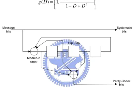
(13) Chapter 2. 5/40. connections in the encoder. To be specific, the generator polynomial of the ith path is defined by. g (i ) ( D) = g 0(i ) + g1(i ) D + g 2(i ) D 2 + L + g v(i ) D v where D denotes the unit-delay variable. In normal cases, the coefficients equal 0 or 1 representative of the connections. However, the short constraint length recursive systematic convolutional (RSC) [10] codes used in turbo codes are not the case. The coefficients of generator polynomial of RSC will be fractional numbers instead of 0 or 1. Figure 2.3 is the example of recursive systematic polynomial whose generator matrix is described as below. ⎡ 1 + D + D2 + D3 ⎤ g ( D) = ⎢1, ⎥ 1 + D + D3 ⎦ ⎣. Figure 2.3 Example of recursive systematic convolutional (RSC) encoder. The reason for making the convolutional codes recursive (i.e., feeding one or more of the tap outputs back to the input) is to make the internal state of the shift register depend on past outputs. This affects the behavior of the error patterns whose characteristics and corresponding decoder structure is beyond the discussion of the thesis. In order to distinguish the normal case of convolutional codes to RSC, some names the normal structures as Feedforward Convolutional Codes. In this thesis, we exclude RSC and only discuss feedforward convolutional codes. From here on, without specification, we refer to convolutional codes as feedforward convolutional codes.. 5.

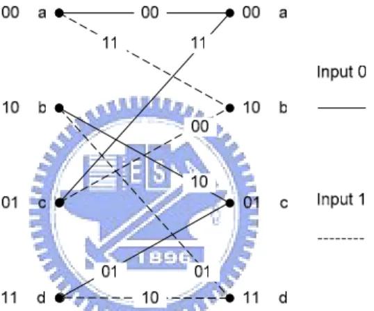
(14) Chapter 2. 6/40. 2.2 Viterbi Decoder. The decoding process could be viewed as the reverse of the encoding process. Often, a trellis diagram will be introduced to help decode since it brings out how the input symbol operates with the contents of shift registers to produce the output symbol. In Figure 2.4, the trellis diagram of a rate 1/2-convolutional code as in Figure 2.1 is displayed. The four states on the trellis represent the possible contents of the registers. For general case in digital system, the number of states equals N=2v. With the trellis diagram, what a decoder has to do is to find the closest match between received signal sequence and the estimated sequence. The most instinctive way to realize the task is brutal search, which is to list all the possible signal sequence combinations and then compare them with the received sequence. At last, take the maximum likely (ML) one as the estimation of the transmitted signal sequence.. Figure 2.4 Trellis diagram for rate 1/2-convolutional code. However, brutal search is never an efficient method. Thus, Viterbi Algorithm was proposed to eliminate the unnecessary comparisons made in the decoding process. Let m denote a message vector and c denote the corresponding code vector applied by the encoder to the input of a discrete memoryless channel. Let r denote the received vector, which may differ from the transmitted code vector due to channel noise. Given the received vector r, the decoder is required to make an estimate of the message vector. Since there is only one-to-one correspondence between the message vector m and the code vector c, the decoder may equivalently produce an estimate of the code vector. Thus, the decoding rule is to choose the estimate of code vector, given the received vector r, minimizes the probability of decoding error. The maximum likelihood decoder or decision rule is described as follow: Choose the estimate cˆ for which the log-likelihood function log p(r | c) is maximum. 6.

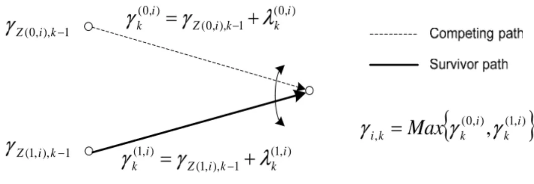
(15) Chapter 2. 7/40. For the binary symmetric channel, the maximum-likelihood decoder reduces to a minimum distance decoder. In such a decoder, the received vector r is compared with each possible transmitted code vector c, and the particular one closest to r is chosen as the correct transmitted code vector. As for the channel with memory, special cares have to be taken in the calculation of likelihood function such as soft decoders [11]. However, no matter which design is chosen, Viterbi algorithm will be applied. The VA recursively finds the most likely path by using a fundamental principle of optimality first introduced by Bellman [12] which we cite here for reference: The Principle of Optimality: An optimal policy has the property that whatever the initial state and initial decision are, the remaining decisions must constitute an optimal policy with regard to the state resulting from the first decision. In the present context of Viterbi decoding, we make use of this principle as follows. If we start accumulating branch metrics along the paths through the trellis, the following observation holds: Whenever two paths merge in one state, only the most likely path (the best path or the survivor path) needs to be retained, since for all possible extensions to these paths, the path which is currently better will always stay better: For any given extension to the paths, both paths are extended by the same branch metrics. This process is described by the add-compare-select (ACS) recursion. The path with the best path metric leading to every state is determined recursively for every step in the trellis. A better elucidation can be made in mathematical expressions. k and i serve only as index here. The metrics of survivor paths for state x k = i at trellis step k are called state metrics γ i,k . In order to determine the state metric γ i,k , we calculate the path metrics for the path leading to state x k = i by adding the state metrics of the predecessor states and the corresponding branch metrics. The predecessor state x k −1 = i for one branch m of the M possible branches where m ∈ {0,1,...M − 1} leading to state x k = i is chosen by the value resulting from evaluation of the state transition function Z ( ) : x k −1 = Z (m, i ) .. γ k( m ,i ) = γ Z ( m ,i ),k −1 + λ(km ,i ) , m ∈ {0,1,...M − 1} where γ k( m,i ) stands for the path metric for a path leading to state s i ,k (state x k = i at trellis step k) and m ∈ {0,1,...M − 1} denotes the path label of one of the M paths leading to state si ,k . The state metric is then determined by selecting the best path. γ i ,k = Max{γ k( 0,i ) , γ k(1,i ) ,..., γ k( M −1, 0) } A sample ACS recursion for one state and M =2 is shown in Figure 2.5. 7.

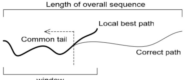
(16) Chapter 2. γ Z ( 0,i ), k −1. γ Z (1, i ), k −1. 8/40. γ k( 0,i ) = γ Z ( 0,i ),k −1 + λ(k0,i ). γ k(1,i ) = γ Z (1,i ), k −1 + λ(k1,i ). γ i , k = Max{γ k( 0,i ) , γ k(1,i ) }. Figure 2.5 Illustration of ACS recursion for M=2 Despite the recursive computation, there are still N=2v best paths pursued by the VA. The maximum likelihood path corresponding to the estimated sequence can be finally determined only after reaching the last state in the trellis. In order to finally retrieve this path and the corresponding sequence of information symbols, either the sequences of information symbols or the sequences of ACS decisions corresponding to each of the N survivor paths for all states i and all trellis steps k have to be stored in the survivor memory unit (SMU) while calculating the ACS recursion. The detailed description of SMU will be provided later in Section 2.4. So far, we considered only the case that the trellis diagram is terminated, i.e. the start and end states are known. If the trellis is terminated, a final decision on the overall best path is possible only at the very end of the trellis. The decoding latency for the VA is then proportional to the length of the trellis. Additionally, the size of the memory element in SMU grows linearly with the length of the trellis. Finally, in applications like broadcasting, a continuous sequence of information bits has to be decoded rather than a terminated sequence, i.e. no known start and end state exists. That is to say that the required length of memory length in SMU has to be at least equal to the length of entire signal sequence. This is wasteful and unpractical in the hardware implementation. Fortunately, through theoretical demonstration and simulations by many researchers, they find that a value of 4 or 5 times the code constraint length K is sufficient for negligible degradation from optimal performance of the decoder. Since with sufficient length of sequence, common tails as in Figure 2.6 will appear. Even though we do not make our decision at the final point, the path chosen will still converge to the optimal path in the front end of the path. Thus, the decoded sequence could be output sooner than traditional VA and the length of memory element will reduce to only 4 or 5 times the constraint length.. 8.

(17) Chapter 2. 9/40. Figure 2.6 The generation of common tail. Figure 2.7 The entire Viterbi Decoder block diagram Summarizing, the basic units of a Viterbi Decoder are shown in Figure 2.7. The branch metrics are calculated from the received symbols in the Branch Metric Generator (BMG). These branch metrics are fed into the add-compare-select unit (ACS), which performs the ACS recursion for all states. The decisions generated in the ACS unit are stored and retrieved in the Survivor Memory Unit (SMU) in order to finally decode the source bits at decision unit (DU) along the final survivor path. 2.4 Survivor Memory Unit (SMU) As we mentioned in the Chapter 1, there are many modified ACS methods invented for the improvements of decoding speed. The price they paid is the need of extra hardware. However, with an expectation of improvement in both decoding efficiency and hardware complexity, we turn our target to survivor memory unit. Thus, in this section, three conventional methods of SMU realization will be provided as basis for the later research. These three methods are traceback management (TBM), register exchange algorithm (REA) and the Hybrid method. 2.4.1 Traceback Management (TBM) In the traceback management, the decision value vectors di [7, 13] and branch label vectors ui (Or previous states), the outputs of ACS, of the S most recent trellis stages are stored. As was explained earlier, in principle all paths that are associated with the 9.

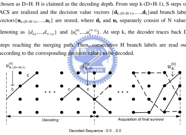
(18) Chapter 2. 10/40. trellis states at a certain time step k have to be reconstructed until they all have merged to find the final survivor path and thus decode the information. However, in practice only one path is reconstructed and the associated information at trellis step k-D output. D must be chosen such that all paths have merged with sufficiently high probability. If D is chosen too small, substantial performance degradations result. As mentioned, the survivor depth D equal to 4 to 5 time constraint length is appropriate for the appearance of common tail. Thus, S has be chosen larger than D. The decoding is then performed by starting at a certain time step k and the tracing back D steps for the assurance of appearance of the merging path. The traceback is then continued from this state and the previous state labels are read out and then to decode out the original data. The above explanation could be illustrated much better in the Figure 2.8. Here, S is chosen as D+H. H is claimed as the decoding depth. From step k-(D+H-1), S steps of ACS are realized and the decision value vectors {dk-(D+H-1),….,dk}and branch label vectors{uk-(D+H-1),….,uk} are stored, where dk and uk separately consist of N values denoting as {d0,k ,...,d N −1,k } and {uk[0] ,...,uk[ N −1] } . At step k, the decoder traces back D steps reaching the merging path. Then, consecutive H branch labels are read out according to the corresponding decision values to be decoded.. u[0] K -(D+ M-1). u [0] K -D. u [0] K. Figure 2.8 Example of TBA Formally, TBA could be stated in a form similar as C language as follows: Memory: (D +H) *N decision bits {dk-(D+H-1),….,dk} stand for upper or lower path Algorithm: // every H trellis steps a trace back is started if (k-D can be divided by H) then { 10.

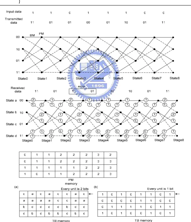
(19) Chapter 2. 11/40. // Initialization traceState := startState ; // Acquisition for t=k downto k-D+1 { traceState := Z(dtraceState,t ,traceState) ; } // Decoding for t=k-D downto k-D-M+1 { decode bit vector := u(dtraceState,t ,traceState) ; traceState := Z(dtraceState,t,traceState) ;} }. Figure 2.9 Different TB memory contents (a) previous states (b) decision values 11.

(20) Chapter 2. 12/40. An example of TBM storing previous states or decision values according to a certain trellis flow is provided above in Figure 2.9, which will serve as a common example for the later comparisons. As seen in the figure, we define the decision value 0 representing the upper path and 1 for the lower path. Before leaving TBM for REA, we have to point out that TBM could be realized with small power consumption and circuit area since there are few logic elements needed. However, it suffers long latency since the decoder has to read in the signal sequence of sufficient length and then feed it into ACS unit. Afterwards, traceback has to be realized for the final decoded output. Therefore, the biggest drawback of TBM is its large latency as well as low decoding efficiency. 2.4.2 Register Exchange Algorithm (REA) The major reason for the development of REA is to improve the drawback of large latency of TBM. Its goal is that the decoded output could be ready right after the ACS of a sufficient length of signals is done. In the register exchange algorithm, survivor paths are stored in N shift registers, each of length S ≧ D. The connection of the multiplexers and registers is derived from the trellis diagram which is constructed by repeating one row containing all states of the code several times to represent consecutive time-steps. By updating the entire contents of every shift register during every decoding cycle (one decoding cycle corresponds to processing one trellis stage), each shift register i always holds the survivor sequence for state i. The decoded data can be obtained from the output of the shift registers. In order to illustrate REA, new parameters should be introduced. We denotes. ) branch labels associated with the path belonging to state i at trellis step k as u k[i ] , with the hat to distinguish from TBM. The branch label associated with the mth branch merging into state i as u ( m,i ) . Thus, we can formally state the algorithm as follows:. Memory:. ) ) (D +1) *N branch labels ( u k[i ] ,…, u k[i−]D ) Algorithm: // Update of the stored symbol sequences according to // the current decision bits di,k (decision bit of state i at step k) for t=k-D to k-1 { for State=0 to N-1 { ) ) [ Z ( d , State )] u k[State ] = u t +1 state , k ;} 12.

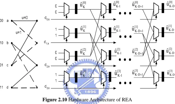
(21) Chapter 2. 13/40. } // setting the first information symbol of the path for State=0 to N-1 { ) [( d , State )] ; u k[State ] = u State , k. } The corresponding hardware implementation of REA is provided as below.. uˆ [0] K. uˆ [0] K -1. uˆ[0] K - D +1. uˆ [0] K -D. uˆ [1] K. uˆ[1] K -1. uˆ [1] K - D +1. uˆ [1] K -D. uˆ [2] K. uˆ [2] K -1. uˆ [2] K - D +1. uˆ [2] K -D. uˆ [3] K. uˆ [3] K -1. uˆ [3] K - D +1. uˆ[3] K -D. Figure 2.10 Hardware Architecture of REA REA successfully reduces the decoding latency. However, when the constraint length increases, REA becomes critical in terms of area and power dissipation. The register exchange algorithm needs the same number of multiplexers and registers as the number of states (N) multiplied by the survivor path length (S) and they are activated every cycle to update data in memory. Thus, REA is mostly applied if latency or total memory size is critical. 2.4.3 The Hybrid method REA is a direct implementation whose critical path consists of one multiplexers and one latch, thus allowing high data throughput. However, area and power consumption rapidly become a critical concern as constraint length grows. TBM, based on RAM, achieve low power and small circuit area but leads to high latency and low throughput. These drawbacks motivated the former researchers to find the balance point. The hybrid method [13,14] was thus developed. 13.

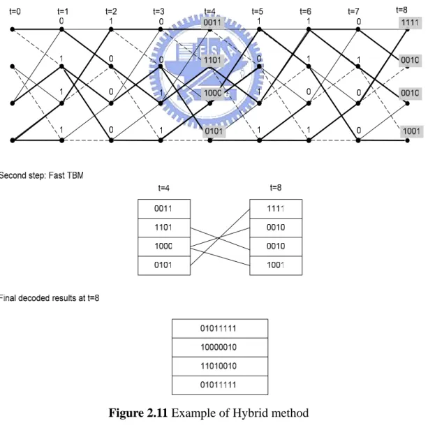
(22) Chapter 2. 14/40. The underlying idea of the Hybrid method is as follows. A continuous exchange registers carried out the whole surviving path leads to unacceptable area and power dissipation. It is nevertheless possible to perform a partial REA that generates segments of survivor paths. After results of partial REA are produced, theses segments of survivor paths are stored in a memory space till sequence of survivor path length S is processed. The fast TBM can then be executed since only a few steps of traceback are required. By doing so, the reduced REA becomes acceptable in area and power consumption and high latency in TBM could be improved. An example is given below in Figure 2.11. The survivor path length (S) is determined as 8, however, partial REA of length 4 is applied. Therefore, the results generated at t=4 and t=8 should be saved as well as the pointer of the previous states. Until t=8, the fast TBM could be realized with only one-step traceback. Detailed computation of the required hardware and latency will be given in Chapter 3.. Figure 2.11 Example of Hybrid method 14.

(23) Chapter 2. 15/40. 2.5 Summary of the Chapter In this chapter, convolutional encoders and Viterbi decoders are introduced. We put more emphasis on the architecture of Viterbi decoders, especially survivor memory unit (SMU). Three conventional methods used to implement SMU are illustrated. TBM has the drawbacks of low throughput and high latency. REA requires larger area and power for multiplexers and exchange registers. These flaws in the two methods motivate us to research for the improved techniques. Even though the Hybrid method had attempted to balance the area/efficiency trade-off, we believe that the hardware could be further reduced. Thus, three improved methods corresponding to the three conventional implementation techniques will be the highlight of the next chapter.. 15.

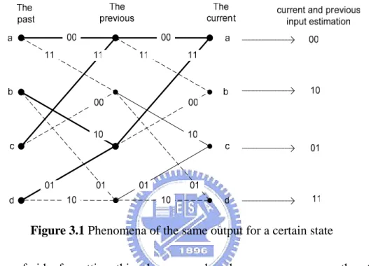
(24) Chapter 3. 16/40. Chapter 3. Three Improved SMU Designs 3.1 Overview As mentioned in Chapter 2, the existing methods in implementing SMU such as TBM and REA fall victims to different flaws. Thus, in the Chapter 3, we aim to derive the new designs that could improve low decoding efficiency of TBM and reduce some memory space as well. On the other hand, for REA and the Hybrid method, the amelioration will be mainly made in the reduction of hardware requirements. These improved SMU designs are all originated from a concept that was aroused by an interesting observation. 3.2 The observation A feedforward convolutional coder is the encoder structure with no feedback loops. As in Figure 2.1, no feedback lines are drawn back to any of the registers. By examining all the possible inputs and register states, the corresponding trellis diagram of the coder could be generated as in Figure 2.4. With trellis diagram, the VA decoder could follow the prescribed paths to finish Add-Compare-Select (ACS) and then choose one ML path as the final estimation. When a path is chosen at last, trace-back has to be done to read out the estimated input sequence. It is a process of mapping from present states to previous states on the trellis diagram and then decides what input symbol the segment represents. In most cases, only one step of trellis diagram will be provided and used in the trace-back process, since pattern of every step in trellis is actually the same. However, when observation is made on a two-step trellis for a (2,1,2) code as in Figure 3.1, one interesting phenomena is found. For convenience of better explanation, we take the rightmost step as the present step and the steps followed to the left are the past steps. When decoding, we used to and have to know states of both the present and the previous steps to decode out only one input symbol. However, by observing the two-step trellis diagram, we find that even though the previous states are unknown. The decoded output is certain for every present state. That is, assuming the present state is a, there are two possible paths from the previous states a and c. Yet, these two paths represent the same input 0. Not merely so, if we trace further back to one more step, four possible paths will 16.

(25) Chapter 3. 17/40. lead to the previous state a and c. Therefore, it makes totally four paths form the leftmost step to the rightmost state a. These four paths stand for the uncertainty and the necessity of trace-back. However, if we look closer, these four paths generate the same two-bit output 00. This explains to us that with mere the knowledge of the present state, we could decode two output symbols in block. The corresponding two-bits output for each of the present states are listed in Figure 3.1.. Figure 3.1 Phenomena of the same output for a certain state Being afraid of spotting this phenomena by chance, we exam another trellis diagram of a rate-1/2 code with v=3. It means that the encoder structure consist of three registers. The trellis diagram is shown in Figure 3.2. From the leftmost step to rightmost step, there are 23 = 8 possible paths converging into the state a of the current step. However, by tracing back the eight different paths, they all lead to the same three-bit output 000. The same experiment could be made on the state b to obtain the three-bit output 010 or randomly selected state e corresponding to three-bit output 100. Namely, by merely knowing the present state, we could decode three symbols out in block, and states in the middle could be neglected. This occurs to us that in the SMU stage, signals can be processed in block. By doing so, we could now decode out more than one symbol a time. An explanation of this phenomenon resulted from the observations might be needed, before we go on the discussion. It is quite easy to unveil the puzzle. We take use of state information to decode signals in block. Therefore, the key should be laid behind the meaning of states. It is obvious to know that states in trellis shows the content stored in registers. This is what we certainly noticed. However, it is easy to ignore what are stored in the registers. They are actually the decoded present and previous input signals. 17.

(26) Chapter 3. 18/40. Figure 3.2 Three-step Trellis for a (2,1,3) code Conclusively, from the observations, we find that a state compose of multiple input symbols. Therefore, it is easy to expect that hardware could be reduced since the states in some steps are needless to be saved. Also, the decoding efficiency should be raised since multiple decoded symbols could be acquired by reading a current state. Three improved SMU designs are evolved from the concept and will be discussed in the following sections. Before going into the next section, one point we have to make clear first is the use of the term “stage” and “step”. In the Chapter 2, while explaining trellis diagram with dimension of time, we refer to step with a specified time parameter such as step t = 4. Without the specification of time, we often use stage in the trellis diagram such as the next stage. However, in the thesis, these two words are used alternatively without discernment. 3.3 Stage-Hopping TBM (SH-TBM) Conventionally in TBM, survivor states have to be recorded every stage and the traceback operation has to be done one stage after another, since it is the relationship between the current and previous states help decipher one input symbol. However, if smaller memory size is desired, obviously state information of some stages will have 18.

(27) Chapter 3. 19/40. to be neglected. Thus, we expect that there does exist some redundant stages and even without them traceback could still be complete. Fortunately, for decoding of general convolution encoders with no feedback loops, we find that the redundant stages do appear for further usage. We have known the fact that, from the previous section, multiple input symbols could be read out by merely knowing one survivor state of a single stage. Since a state could tell us what the current and previous input symbols are, the stages in the middle are not necessarily stored. For general coder schemes, a parameter named BS (block size) has to be well defined to indicate how many stages traceback could hop over at once. It is obvious to see that for the encoder schemes with only a string of registers as in Figure 2.1, a state contains the same number of input symbols as the number of registers. However, for the encoders with more than one string of registers as in Figure 2.2, the string with least number of registers will dominate the definition. It is due to the fact that the input symbols will be drop out for the unequal length of registers in different strings. Therefore, a sound definition of the BS should be: BS = Max{ Min{NRn , n ≤ NS }, 1 }. where NRn stands for the number of registers in the nth string and NS represents the number of overall register strings. BS indicates two important facts: one is the number of input symbols that could be read out by one state, and the other is the number of stages that traceback could hop over once. Hence, the task left to be solved now is how to eliminate the redundant stages in between and reserve only the needed survivor states that are every BS stages away to carry on traceback. Figure 3.3(a) shows the conventional memory management technique for the (2,1,2) code. We can see that every survivor state in different paths is well stored in the memory. Even though the input could still be decoded out correctly as 0011 by knowing the current state a and state d that is two-stage away, we could not directly neglect previous state c, since trace-back may not be carried on without the link to state d. Therefore, we shall not just get rid of contents in memory but should take the strategy of updating memory as in Figure 3.3(b). The update procedure provided here is just a guideline for implementation. Actually, as long as the right survivor states every BS away are stored, the profit of memory reduction could still be gained for TBM. The overall procedure could be divided into six steps:. 19.

(28) Chapter 3. 20/40. Step 1: Check BS is even or odd. Step 2: If it is even, then start by storing survivor states in the extra temporary row of memory. Else, if it is odd, start by storing survivor states in the original memory space. Step 3: At the beginning of every block, the survivor states will be stored into the assigned row of memory after ACS process. Step 4: For the rest signals from the same block, the newly selected survivor will not be stored. Instead, it will be used as an indicator to copy the data, which it is pointed to, to the other row of memory iteratively. Step 5: Repeat step 1~4 until the entire sequence is processed. Step 6: Traceback and decode output block-by-block. Figure 3.3 The procedure of Stage-Hopping TBM In this way, as we can see in Figure 3.3(c), half of memory size could be saved at last. As for general convolution coders, only one-BSth of the conventional memory size is required. Since for a block of survivor states, only one survivor state is saved at last. In conclusion, Stage-Hopping TBM takes use of the fact that multiple input symbols could be read out by merely knowing one survivor state so as to eliminate the necessity of storing those redundant stages in between with updating states skills. 20.

(29) Chapter 3. 21/40. By doing so, memory used to save survivor paths could be reduced. In addition, decoding efficiency could be greatly improved as an important value of the method due to the fact that fewer stages remained to realize traceback operation. A detailed computation of the decoding efficiency and the required memory size will be given later in Chapter 4 to make the overall comparisons. 3.4 Facilitated REA (FREA) REA uses a direct hardware implementation of the trellis structure. Survivor states are stored in N shift register and each shift register i always holds the survivor state for state i. The traceback operation of TBM is replaced by updating the entire contents of every shift register during every decoding cycle to obtain high throughput and low latency. However, as constraint length grows, the area and power dissipation increase quickly. As a result, it will be less preferable to be applied with a large number of states in the trellis or with long constraint length. The concept of the improvement is the same as Stage-Hopping TBM. Basically, the FREA could be considered as using exchange register technique to implement the six- step procedure mentioned in the Stage-Hopping TBM. However, direct conversion may be problematic. First, contents stored in memory of SH-TBM are previous state information which is different from the decision values in REA method. Luckily, the problem can be easily solved that the state information stored is actually the decoded data, which is even more desirable to acquire. Second, the REA continuously recorded the previous state information. On the other hand, only those survivor states every BS away are needed to be solved. Therefore, the design should be adjusted to execute the correct procedure. Before constructing the overall FREA, the elementary structure is our first target to realize. Since only survivor states every BS away are necessary to be stored. The recursive manner should be applied on the elementary structure as shown in Figure 3.4. As we marked on the figure, there are three differences from the conventional REA design. (1) The feedback line is drawn to replace the original data stored in the register so that only survivor states every BS cycles will be recorded and those states in the middle stages will be surpassed. (2) The set_inital signal is active every BS cycle as a signal to restore the content of registers. This will be explained more in the entire FREA design. (3) Decision values are only fed into MUX and do not write in the registers. An easy example is given in Figure 3.5 where a two-step trellis is formed. The necessary survivor states (0,3,2,0) are stored at last by SH-TBM. The equivalent functions of elementary component of FREA is provided in the lower part of the Figure 3.5 which generates the same results at t =2. 21.

(30) Chapter 3. 22/40. Figure 3.4 Elementary component structure of the FREA method. Figure 3.5 Equivalent function of SH-TBM and the elementary component of REA. 22.

(31) Chapter 3. 23/40. From the above, we should somehow sense that the number of multiplexers used in the FREA is less than that required in REA since the multiple steps of trellis are processed by a single column of multiplexers. To construct the entire FREA, the elementary components have to be well connected, where some tricks are applied to make the FREA function properly. The overall hardware structure of FREA is shown in Figure 3.6 in the next page. The tricks lie in the use of set_initial signal to control the contents of registers. (1)At leftmost stage, when the set_initial is active, the register will be set into default value as (0,1,2,3) for the selection of survivor states of the latest stage. (2) As for the rest of registers, the contents of the registers will be past to the next stage after BS cycles, set_initial is active, so that contents of register i will always save the survivor state that is BS-step away for the state i on the same survival path. Originally, in REA, the number of multiplexers required is equal to N (the number of states) *S (the length of survivor path). With FREA, BS states can be iteratively allocated by only one column of multiplexers, so only N*S/BS multiplexers are needed. In addition, decision unit is no longer required since state information already represents the decoded input symbols. Moreover, the wire connections can have fewer crossings. These improvements will not only reduce the required hardware but facilitate the implementation of SMU. Details of the required number of multiplexers and decoding efficiency will be provided in the Chapter 4 later. 3.5 Improved Hybrid Method (IHY) With the previous introduction of the Hybrid method and Stage-Hopping TBM, one might find that the improved decoding efficiency of SH-TBM is the same as the decoding efficiency of the Hybrid method when the partial REA of length BS is applied. However, the better decoding efficiency of the Hybrid method is obtained at the cost of lot more hardware than SH-TBM. To implement the Hybrid method, memory used to store survivor states is required. Besides, multiplexers and registers are also necessary for the partial REA. Therefore, there are still some rooms left for improvements of the Hybrid method. We name it Improved Hybrid (IHY) method. The first improvement is directly inherited from the FREA. That is, when the partial REA is implemented, we could modify it into the FREA structure so that the number of multiplexers could be reduced. The structure is the same as in Figure 3.5 and 3.6. A little difference between Hybrid method and IHY is that the length of partial REA should be always chosen as the constant multiple of BS so that FREA could be easily constructed. If the length of signals is not so, some measurements as zero-stuffing or eliminating the unwanted output signals should be taken. 23.

(32) Chapter 3. 24/40. Figure 3.6 The hardware structure of FREA 24.

(33) Chapter 3. 25/40. The second improvement is lying on the traceback and decision procedure. In the conventional Hybrid method [14,15], traceback has to be assisted with previous state information which may be saved in a lookup table and make the decision of the input symbol in the decision unit. In the IHY, a state plays two roles. One is the previous state information and the other is the decoded data. Thus, the traceback and decision could be operated easily with some multiplexers. An example is given as in the Figure 3.7. BS of the coder is 2 and the partial REA length is 4. Thus, the 4-bit output of partial REA will be sequentially stored in the memory. When tracing back, the last 2 bits of the 4-bit output could serve as the indicator of the previous state so that the traceback and decision operated could be mixed up and implemented easily.. Figure 3.7 Example of the mixed traceback and decision operations 3.6 Summary of the Chapter In this Chapter, three improved methods of implementing SMU are proposed. Stage-Hopping TBM (SH-TBM) is proposed to improve the drawbacks of low decoding efficiency without the cost of any extra hardware; instead, it could further reduce the required memory space. Facilitated REA (FREA) and Improved Hybrid method (IHY) are brought up to decrease the required number of multiplexers so that the drawback of large circuit area could be ameliorated. Of all three improved methods, decision unit (DU) is no longer needed since states stored in the memory are equivalent to the storage of decoded data.. 25.

(34) Chapter 4. 26/40. Chapter 4. Experimental Results and Analysis 4.1 Decoding performance In the previous chapter, we have demonstrated how the improved methods are developed to reduce the hardware complexity and increase the decoding efficiency. However, one may question if the decoding performance is sacrificed. Therefore, the first thing we want to verify is the decoding performance. At first, we simulate the rate-1/2 code with v=6, which is the inner channel coder of DVB-T system, by C++ program. The input generated is random binary signals, the channel is AWGN and the receiver is soft Viterbi decoder. The experimental results are shown in Table I. In Table I, case 1 uses conventional TBM with memory length that is equal to 5 times constraint length which guarantee the generation of common tail. Case 2 uses 10 times constraint length which has longer decoding depth and case 3 applies SH-TBM whose memory length equals to 10 times constraint length dividing by BS=6. Though case 3 intrinsically executes SH-TBM, it can also represent the decoding performance of FREA and IHY since they are based on the same concept with different hardware designs. We can see in table that longer survivor path seems to produce a little better decoding performance from the comparison between case 1 and case 2. From case 2 and case 3, we successfully prove that three newly proposed survivor memory management methods of SMU do not degrade the decoding performance. On the contrary, some additional advantages could be acquired. Table I. Performance of Viterbi Decoder with different memory management techniques of SMU SNR / BER. Case 1. Case 2. Case 3. 0dB. 0.168584. 0.155538. 0.152853334. 0.5dB. 0.095194. 0.088226. 0.088806667. 1dB. 0.04808. 0.0402442. 0.04044. 1.5dB. 0.01883. 0.0158866. 0.01509. 0.006908. 0.0049522. 0.005268. 2.5dB. 0.0018922. 0.0014524. 0.001472333. 3dB. 0.0004536. 0.0003482. 0.000361067. 3.5dB. 0.0000932. 0.00008054. 8.30666E-05. 0.000018504. 0.000015188. 1.61136E-05. 2dB. 4dB. 26.

(35) Chapter 4. 27/40. 4.2 Decoding efficiency and Hardware Reduction In this section, graphical method is introduced to illustrate the decoding efficiency and the required memory size of three conventional methods and three corresponding improved methods for comparisons. The reason of using graphical method is to carefully estimate the decoding efficiency and memory size in real hardware implementations instead of the mathematic calculations, used in software simulations, given as in previous chapters. 4.2.1 TBM vs. Stage-Hopping TBM (1) TBM. Latency. 4D Write-Decisions Acquisition-Trace Data-Trace. 3D. M1 M5. 2D. M4 M3. D. M2 M1. D. 2D. 3D. 4D. Time ( Clock-Cycles). Figure 4.1 Graphic representation of a conventional TBM The decoding cycle refers to the generation time for a decision vector computed by ACS unit and is also equal to the duration of one traceback. Length of the survivor path (S) is chosen as D (sufficient length of signals to create common tail) + H (decoding depth). H here is selected as 0.5D. From t=0 to 1.5D, decision vectors are generated by ACS units. Till then, a survivor path is chosen and follows on a depth D+H traceback, in order to get H decoded data. In the figure, TB memory represents the memory used to save states on the survivor paths or the decision vectors of every stage. From the figure, we could make an overall analysis as follows: 27.

(36) Chapter 4. 28/40. Table II. Analysis of TBM In the example. In general case. TB memory (R/W). (1.5D+D)*N=2.5*D*N. (D+H+D)*N= 2*D*N. TB memory. 1.5D*2*N=3*D*N. (D+H)*2*N=2*(D+H)*N. Latency. 3*D. 2*(D+H). Decoding Efficiency. 0.5D/3D =1/6. H/(H+D+H)=H/(D+2*H). where R/W means that memory could finish read and write in one cycle and the unit of TB memory is symbols. (2) Stage-Hopping TBM ( I ) Software Implementation Though the states only BS steps away are necessary to be stored, the memory size do not reduce as expected compared with decision value method. Since it only uses one-bit decision value to record the upper or lower path, we find that the TB memory size is actually the same as shown in Figure 4.2, which are the results of the example given in Figure 2.9 by decision value method and SH-TBM. However, decision value method still requires state memory table and decision data lookup table to read out the previous state and decode. Hence, there is still certain amount of memory reduction gained by eliminating the need of state memory and decoded data lookup table in SH-TBM. The new decoder design could be drawn as in Figure 4.3.. Figure 4.2 Required memory size of decision value method and SH-TBM One might be disappointed by the results. Luckily, it is a totally different story when it is implemented on real hardware. Since there is no reason to separate ACS and traceback operation, the ACS should still be under process while tracing back in 28.

(37) Chapter 4. 29/40. SMU. Hence, the memory needed to store the results of ACS will be related to the duration of traceback. That is to say that the longer time the traceback requires, the larger memory the SMU needs. More details will be illustrated by graphic representation and lot more discussion in memory reduction will be provided later.. Figure 4.3 TBM decoder design and SH-TBM decoder design (II) Hardware Implementation H is chosen the same as 0.5D and BS here is assumed to be 2. At first, D+0.5D data are read in and create the corresponding decision vectors after ACS units. The major differences come in the phase of traceback and decoding. In the traceback, the speed is increased since fewer stages are left to be traced and a state can now output two decoded symbols at a clock so that H decoded data could be acquire faster. In the Figure 4.4, we could see that the slope of the acquisition and data-trace lines is –BS.. Figure 4.4 Graphic representation of SH-TBM 29.

(38) Chapter 4. 30/40. Table III. Analysis of SH-TBM In the example. In general case. TB memory (R/W). (1.5D+D/BS)*N=2*D*N. (D+H+D/BS)*N. TB memory. [1.5D+(1.5D/BS)]*N=2.25*D*N [(D+H)+(D+H)/BS]*N. Latency. 2.25*D. (D+H)+(D+H)/BS. Decoding Efficiency. 0.5D/2.25D =1/4.5. H/[H+(D+H)/BS]. (3) Comparisons H itself is a trade-off factor when it comes to TBM. The longer the decoding path is, the larger the latency or decoding efficiency is. However, if the H is chosen to be small, the memory intensity will be low and control signals will be more sophisticated. This issue will be overlooked in the research. In the later discussion, we will fix H as a constant parameter. (a) Decoding Efficiency and Latency We can see that the decoding latency of Stage-Hopping TBM is D+H+(D+H)/BS. D is often chosen as 4 to 5 times constraint length. BS for the (n,1,v) code is the same as v = K-1. This indicates the fact that the traceback operation can now be realized in only a few clock cycles (D+H)/BS. It will be more obvious to see in the decoding efficiency. The improved decoding efficiency is H/[H+(D+H)/BS]. As the BS grows, the decoding efficiency could be improved much better approaching to the performance of REA. The improvement of decoding efficiency is also shown below in the Figure 4.5, with D = 5v and H = v. We have to emphasize that the decoding efficiency improvement is gained without extra hardware, and even more the memory size is further reduced, which will be explained next.. Figure 4.5 Decoding Efficiency of TBM and SH-TBM 30.

(39) Chapter 4. 31/40. (b) Memory reduction in hardware implementation 1 1 ) (1 − ) 1 BS BS Memory reduction ratio is computed as ∝ (1 − = ) . That H D+H +D BS +2 D D(1 −. is as constraint length increases the memory space used to save survivor sequence will be much smaller in SH-TBM than in conventional TBM. As for (n,1,v) code, BS is equal to v and assume D=5v, H=v. We can see the memory reduction curve as in Figure 4.6. About 5/11≒45% of original TB memory can be saved at most. Besides, decision unit (DU) is no longer needed. Thus, hardware could be further reduced.. Figure 4.6 Memory reduction ratios 4.2.2 REA vs. Facilitated REA. Figure 4.7 Graphic representations of REA and FREA 31.

(40) Chapter 4. 32/40. Figure 4.8 Different register allocations of REA and FREA Table IV. Analysis between REA and FREA REA. FREA. overall size of registers. N*D. N*D. number of MUXs. N*D. N*D/BS. Latency. D. D. Decoding Efficiency. 1. 1. where the unit of size of registers is symbols Figure 4.7 represents both REA and FREA, since the only difference in them is the hardware implementation. There are two modifications demanded for explanations: (a) The overall size of registers In conventional REA, the unit of one register is one-bit decision value. On the other hand, the unit of one register is BS bits, since content of registers has to be overwritten. However, one register in FREA will be repeatedly utilized BS times before it transmits its content to the next register so that the overall size of registers is actually the same, which is illustrated as in Figure 4.8 with BS =3. (b) The number of Multiplexers The major advantage of FREA is the reduction of multiplexers. Compared with REA, multiplexers used in FREA are still two-to-one multiplexers. The complexity of multiplexer remains the same. However, since only the state information that is BS steps away is required, a multiplexer can be used repeatedly until state of the correct previous step is acquired. Thus, we can say that only one-BSth of multiplexers in REA are needed to realize the same task. More analyses are listed in Table IV. So far, we have only displayed the comparisons of hardware requirements between REA and FREA. Without implementation of the FREA, one might render the method doubtful. Therefore, we do implement the elementary component as described in Figure 3.4 and send in the decision vectors as in Figure 3.5 to observe the result. 32.

(41) Chapter 4. 33/40. The entire VLSI program for the elementary component of FREA and its test file are listed in the appendix A. The simulation result is now shown as follows:. Figure 4.9 Simulation results of elementary component of FREA We can see that as the decision vector [0,0,0,1] generated from ACS outputs, the contents of registers become [0,2,0,3]. At the next clock cycle, new decision vector is formed as [0,1,1,0] and lead to the record of [0,3,2,0] in the registers. The result matches with the description in the Figure 3.5. Thus, we could now validate the correctness of the function of the elementary component. 4.2.3 Hybrid method vs. Improved Hybrid method (IHY). Figure 4.10 Graphic representation of Hybrid method 33.

(42) Chapter 4. 34/40. Figure 4.11 Graphic representation of IHY Inherited from SH-TBM and FREA, we can daringly expect the same degree of reduction in the number of multiplexers and memory. In addition, IHY can decode out input symbols a little faster since it could read out multiple symbols a time. Graphic representations as Figure 4.10 and 4.11 could display these improvements more clearly. The Hybrid method has improved the speed of acquisition trace by using partial REA of length 2. However, the data trace still has to be done one symbol after another. A slight increase of decoding efficiency can be gained at data-trace since two symbols can be read out once in IHY when its BS equal to two. Due to the faster traceback time, some of the TB memory could be saved. Besides, most important of all, the number of multiplexers could be reduced by BS. For the case when the length of partial REA equals to BS, only a column of multiplexers are needed. This makes the implementation easier and the required hardware area smaller. Table V. Analysis between Hybrid method and Improved Hybrid method Hybrid method. Improved Hybrid method. TB memory (R/W). (D+H+D/Dp)*N. (D+H+D/Dp)*N. TB memory. [D+H+D/Dp+H]*N. [D+H+(D+H)/Dp]*N. Number of MUXs. N*Dp. N*Dp /BS. Latency. D+H+D/Dp+H. D+H+(D+H)/Dp. Decoding Efficiency. H/(H+D/Dp+H). H/(H+(D+H)/Dp) 34.

(43) Chapter 4. 35/40. 4.3 Power dissipation and Summary of the Chapter Though we do not measure the real power dissipation of the improved methods, we could still approximately estimate their relativity. First, TBM and SH-TBM consumes the lowest power. IHY could save a little power since fewer multiplexers are turned on than Hybrid method. REA requires the largest power since multiplexers and registers have to remain active in every cycle. The reduction of multiplexers in FREA should make it dissipate less power. An overall estimation is as followed: ◎ Power: T=SH<IH<H<FR<R ◎ Hardware: SH≦T<IH≦H<FR≦R ◎ Throughput: T≦SH<IH≦H<R=FR. ( T:TBM, SH: SH-TBM, H: Hybrid, IH: IHY, R:REA,FR:FREA). 35.

(44) Chapter 5. 36/40. Chapter 5. Conclusion 5.1 Conclusion Motivated by the desire of improving the existing implementation methods of SMU in Viterbi Decoder, we start by observing trellis diagram of some commonly used convolutional coders. From the trellis diagrams, we found an important concept that state information contains multiple input symbols for feedforward convolutional encoders without feedback loop. That is excluding RSC. With the concept, we begin by defining a parameter called BS. It indicates two important facts: one is the number of input symbols that could be read out by one state, and the other is the number of stages that traceback could hop over once. By applying the concept on TBM, Stage-Hopping TBM is then developed. It stores only states that are BS steps away in memory so that the memory size should be reduced. The improved memory size eliminates the need of previous state table and decoded data table compared with decision value method when investigating it by software implementation. On the other hand, by graphic representations, we can see that up to 45% of the original TB memory can be saved for (n,1,v) code in hardware design. Most important of all, the decoding efficiency considered as the major drawback of TBM is improved approaching performance of REA as constraint length increases. Corresponding to REA, Facilitated REA (FREA) is proposed based on the same state information concept to reduce the hardware complexity of REA. REA suffers large circuit area and large power consumption since the huge amount of multiplexers and registers in REA structure are active in every clock cycle. By repeatedly utilizing a column of multiplexers, we reserve only the previous state information that is BS steps away. Therefore, only one-BSth of the original multiplexers is needed. The FREA hardware design is a bit different than the conventional REA. The size of registers, the connection and the extra control signal are modified so that the new design not only makes it function properly and but also reduces the hardware requirements. Combined REA with TBM, the Hybrid method was then generated. Thus, Improved Hybrid (IHY) method will naturally inherit the improvements of StageHopping TBM and Facilitated REA. The number of multiplexers could be reduced and a small amount of memory could be saved. Most important of all, the traceback in IHY could be realized faster and its hardware implementation becomes very 36.

(45) Chapter 5. 37/40. simple that only a few of multiplexers will cut out for the task. Besides, among the three new methods, no decision unit (DU) is needed because states stored already consist of the decoded input symbols. These improvements are gained almost without any cost. Just that the extent of the improvement depends on the structure of the convolutional encoders. Thus, for some systems, there may be no advantage that can be acquired by applying these methods. Even so, without any cost, we should be satisfied with the advantages that these methods could bring to us as long as the encoder allows. Besides, decoders of the punctured convolutional code could also take use of these improved methods. There is actually little limitation in utilizing these new designs. To sum up, we propose three new SMU design for Viterbi decoders. Stage-Hopping method can obtain higher throughput without extra hardware. Furthermore, memory size could be reduced by 45% at most in hardware implementation. On the other hand, FREA improves REA in the reduced number of required multiplexers. At last, IHY inherits both advantages of SH-TBM and FREA so that it can not only improve the Hybrid method in both the reduced number of multiplexers but also acquire the ability to realize faster traceback operation. 5.2 Future work Power dissipations of three new designs mentioned in Chapter 4 are only under logical estimation. The actual measurement of power dissipation may be of help for the designer to choose the customized SMU structures. Other than being applied on the designs of SMU, the concept of state information contains multiple input symbols can be also of use in the joint source-channel decoder designs [16]. The channel decoder could be referred as the course selector for the candidates of source decoder. By doing so, the complexity of entire decoding system should be decreased. This application might worth some more future works.. 37.