Pergamon Copyright 0 1996 Elsevier science Ltd F’rinted in Great Britain. All rights reserved 002&7683(95)00284-7 002&76tl3/% SIS.C’J + .OO
EXACT TRANSIENT SOLUTIONS OF BURIED
DYNAMIC POINT FORCES FOR ELASTIC
BIMATERIALS
CHIEN-CHING MA and IWO-CHENG HUANG
Depafiment of Mechanical Engineering, National Taiwan University, Taipei, Taiwan 10617, Republic of China
(Received 16 May 1995 ; in revisedform 30 October 1995)
Abstract--The exact transient closed form solutions for applying time dependent point forces at a depth below the interface of dissimilar solids are obtained in this study. The problem is solved by application of Laplace transform methods. The inverse transforms are evaluated by means of Cagniard’s method. The equations of wave fronts for reflected and refracted waves induced from the bimatcrial interface by the incident waves are determined in this study. The corresponding static solutions of stresses and displacements are reduced from the obtained transient solutions. Numerical results of stress fields during the transient process are obtained for different cases and compared with the corresponding static values. Copyright 0 1996 Elsevier Science Ltd
INTRODUCTION
The propagation of stress waves through an unbounded medium is not a difficult subject. If a boundary is introduced, however, reflected waves will be generated from the free surface, making the problem more complicated. The classical analysis in this area was first proposed by Lamb (1904), he considered the transient problem of applying dynamic point and line loads on the surface of a semi-infinite half space. Since this early analysis by Lamb, a great many contributions have appeared pertaining to what is commonly referred to as Lamb’s problem. Buried source problems are of practical interest, particularly in the field of seismology, and have been studied by many investigators, including Lamb. Nakano (1925) analyzed the buried line dilatation source in a half space, but he failed in generalizing his harmonic steady state results to transient solutions. Lapwood (1949) re-studied Nak- ano’s problem, and later Garvin (1956) also solved Nakano’s buried line dilatation source problem by msing a suitable distortion of the contour suggested by the work of Cagniard. In Garvin’s paper, the numerical results are limited to surface displacement due to a dilatation source, and the generated waves in the medium are only incident P wave, reflected PP wave and :PS wave.
The three dimensional problem of a buried dynamic vertical point source was studied by Pekeris (1!)55a, 1955b) and Pekeris and Lifson (1957). Pekeris divided the half space into two regions horizontally along the loading position, ancl then applied Laplace and Hankel transforms to solve this problem. From the traction free boundary condition and the continuity requirement at the intersection of the two regions, complicated solutions were represemed in integral form and only the surface displacements were obtained numeri- cally. Based on a similar methodology, Payton (1967, 1968) solved for the displacement on the free surfac:e and on the axial line of a two dimensional half-space subjected to a buried line source. The suddenly applied normal point load which travels on the surface of a half-space wa;s first derived by Gakenheimer and Miklowitz (1969). Laplace and Fourier transforms were employed to solve the problem, and the Cagniard+le Hoop method (1958) was applied to invert the transform.
The complete transient response resulting from applying a dynamic point force and a displacement jump in an arbitrary direction under a two dimensional half space was investigated by Tsai and Ma (1991). The two dimensional static stress distribution due to
point loads applied within the elastic half plane has been solved by Melan (1932). These 4511
4512 Chien-Ching Ma and Kuo-Cheng Huang
solutions were extended and applied to the direct boundary element method for half plane problems by Telles and Brebbia (198 1). The three-dimensional static fundamental solution for the half space has been solved by Mindlin (1936), and its application to the boundary element method has also been established by Nakaguma (1979).
In many situations, waves originate and propagate in media having a layered structure, where interfaces between dissimilar materials exist. Seismic waves in a layered earth are an example, and important applications in structures also exist, such as waves in composite plates. The large class of problems for a simple half-space, such as reflection of plane waves and source problems, now have their more complicated and numerous counterparts in layered media problems. The simplest situation in this area consists of two semi-infinite media in contact. Such a situation, strictly speaking, is not a layered system since neither media possesses two parallel boundaries. Nevertheless, this natural extension of the single, semi-infinite media problem is a pre-requisite to the analysis of layered systems. The solution
of the simplest problem of the propagation and transmission of plane harmonic waves
across the interface between two semi-infinite media is well known. However, the transient analysis for the problem of propagation and transmission of inplane curved waves across the interface is not completely developed yet. In this investigation, the transient response resulting from the application of buried dynamic point forces with arbitrary orientation in a bimaterial interface will be studied in detail. The results presented in this paper are exact and are expressed in a simple closed form, each mathematical term representing a physical transient wave. The corresponding static solutions are obtained by taking appropriate limits of the transient results. The results of the numerical calculations of stress are used to investigate the transient behavior of stress waves propagation in bimaterial medium.
FORMULATION OF THE BOUNDARY-VALUE PROBLEM
Let x and y be a two-dimensional Cartesian coordinate system, oriented as shown in Fig. 1. Solid 1 occupies the region y < 0, and solid 2 occupies the region y > 0, with y = 0 being the common interface. The problem considered in this study is two-dimensional, and the plane strain formulation is employed. The governing equations can be represented by the longitudinal potential 4 and the shear potential tj as follows
V2c$--a2ij = 0,
(1)
V2$-b’$ = 0, (2)
where V2 = a2/ax2 + a2/ay2, and
J
P1
a= -=v,, b=
;=‘.
J
us (3)In (3), a and b are the slownesses of the longitudinal wave and the shear wave, p and p are
Fig. 1. Configuration and coordinate system of a biiterial interface dynamic point force.
the shear modulus and the mass density, and A is the Lame elastic constant, respectively. The displacement and stress can be expressed in terms of the potentials as
a XY =p 2$&3+3. (
(6)
(7)
(8)
For the case where the two media are bonded together, continuity of displacement and traction across the interface is required. Thus, the boundary conditions to be satisfied along the interface y = 0 are :
24,.(x,0, t) = 24,2(x,0, r), --co < x < 03,
(11)
uyl (x, 0, t) = uy2(x, 0, f), - EJ < x < 00.
(12)
This problem can be solved by the application of integral transforms. The one-sided Laplace transform over time and the bilateral Laplace transform on the spatial variable x for a function 4 is defined by
~$(x,y, t) ePP’dtdx
where p is a positive real number, large enough to ensure convergence of the integral, and
1 being a complex variable. The corresponding transforms of the displacements and the stresses are ~,,(AY,P) = PP P(b2
-212hi5-21$
[ -1 3 b,(il,y,p) =pp1
,
~,(AY,P)=
P/J 5d$
+p(b2--2~2)$
1,
(13) (14)(15)
Chien-Ching Ma and Kuo-Cheng Huang 4514
(16)
(17)
To solve the posed problem, we define potentials +i and tii in solids 1 and 2 by
The right sides of (18), (19) are the potentials representing the incident (47, reflected (@), and refracted (@) waves.
SOLUTIONS IN TRANSFORM DOMAIN FOR BURIED POINT SOURCES
Consider two isotropic linear elastic half spaces, which are perfectly bonded along the interface - 00 < x < co. Initially, the bodies are stress free and at rest. At time t = 0, a concentrated dynamic force with arbitrary angle 8 is applied at a distance h under the interface. The geometry and coordinate system for this problem are shown in Fig. 1. The suddenly applied point force may be represented by the following distribution of body forces :
F = -2(sin8i+cos0j)a06(x)6(y+h)H(t), (20)
where 6 is the Dirac delta function and H is the Heaviside step function. Incident fields in the Laplace transform domain can be represented in the form
~VrY,P) = cro T1 (A) e-plIv+hi
p3,G:
’
where
1 Ti(n) = cosf3+ -sin@,
a1
T 2 (A) =
case-
%ineA .
(21)
(22)
The incident fields representing the response from loading applied to an unbounded medium. The reflected and refracted potentials ($‘, v, & fi can be determined such that the tractions and the displacements are continuous across the interface y = 0 and also must satisfy the wave eqns (1) and (2). The results for reflected and refracted potentials in the Laplace transform domain are
4515
q=-_ COT,@) ~I(~)~.,~~_~~+ aoTz(W A5(Q,y_B,h)
p’p, b: R(l) p’,u,b:j3, R(1) ’ co TI (A) A 3 (A) &_-.--e p’p, b: R(A) p@,y-qh) + hT2(W A7(A)egS*(y-h) p’/.i,b:/!?, R(J) ’
aoT1
(2)
40)
(jf =-__e p’p, b: R(J)-p(orzy+ol,,,) + aoT2W
-40)
e-p(a2y+B,,,)p’p,b:/?, R(A) ’ (23) (24)
(25)
W-9
whereR(A) = 4A2ala2B1S2(l -_y)’ +A2[b: -yb3 +2(y- l)A’]’ +y(a,a2 +a2fil)b:b:
+a,B,[yb:+2(1-y)12]2+a2fi2[bf+2(y-1)A2]2, (27) Al(n) =4~2o:,a2~,~2(1-y)2-122[b~-yb~+2(y-1)3L2]2+y(a,~2-a2~l)b~b~ +a,Bl[yb~+2(1-y)12]2-a2fi,[b~+2(y-1)12]2, &(A) = 2a,b:{82[b:+2(y-1)~2]+Bl[yb:+2(1-y)12]}, A3(4 =4;la:,a2B2(1-y)[b:+2(y-1)~2]+21al[-b:+yb:+2(y-1)~2][yb:+2(1-y)12], A4(jl) = 2alIb:{2a2jI,(1-y)-bf+yb:-2(y-1)A2}, -45(l) =4~a2~,P~(l-y)[b~+2(y-1)122]-2~1~[-b~+yb~+2(y-1)~2][yb~+2(1-y)l2], &(A) = -2fi,Ab~(2al~2(l-y)-b~+yb~-2(y-1)A2}, AT(~) =4~2a,a28,B2(1-y)2-j12[b:-yb:+2(y-1)~2]2+y(a2Q,-a,~2)b:b: +a,B,[yb~+2(1-y)12]2-a2fi2[b~+2(y-l)A2]2, As(L) =2/?,b~{a2[b~+2(y-l)12]+a,[yb~+2(1-y)A2]}, in which ai =(a’-;12)1/2, pi =(b?-J2)1’2, i= 1,2, Y = cL2I~~~
The function R(I) in (27) is the characteristic function for Stoneley waves at the
interface of two dissimilar solids. When the solid 2 is absent, the function R(A) in (27) will
reduce to the equation of Rayleigh surface waves. The condition Re ai > 0 (Re #Ii 2 0) is
satisfied by providing branch cuts along ai < 1 Re ;1I < co (pi < 1 Re A 1 c co), Im A= 0, and choosing the branch of positive real parts.
The inverse of the bilateral Laplace transformation is defined in the usual manner.
When we combine eqns (13)-(17), (21)-(26), the solutions for stresses and displacements
in the Laplacic transform domain can be expressed as follows :
8yyl (X, y,p) =
2.
s
{F, (I) e-PaJy+hi+prlx+ F2 (A) ePal(Yph)+Phl-
+F’(J) &m-v)+P~ +1;4(~)e-P~,b’+hi+P~
+F5(A) eP(8,Y--a,h)+Pix + F6 (A) epSl (y--h)+ph} d1,
Chien-Ching Ma and Kuo-Cheng Huang
s
{F:(J) ~--p@zY+~l~)+P~ +jy(A) e-P(w+k%*)+P~ r
Cyl
(x9
y,p) = Zf-
2Ais
.f{G
(4
e-
palIy+hi+P~x+G2(;1) eprr,(y-h)+plx
+G,(A) ep%Y--.th)+Ph + G6(IZ) ep~l(y-h)+pk} dl,
fiy2(X,Y,P) =
“O
2~i s.j {G:(n) e-P(+Y+qh)+Ph +Q@) e-P(azy+8,h)+pk
+ G;(A) e-pCBzY+qh)+PAx + G:(A) e-p@2yt~l*)+PRX) d2,
8xxxl(X,y,p) =
2.
s
{H,(~)e-P”~~Y+h~+P~x+~~(~)eplr~(Y--h)+p~~l-
+~~(;~)~(~IY-~~~)+P~x+~~(~)~-PB,~Y+~I+P~x
+~,(q ep%y--cih)+p~x + H6 (A) epD~(y-h)+p~} dl,
s
{H?(d) e-P(cr2y+alh)+P~ +Hf(;1) e-P(a2Y+Blh)+pk l-
+HT(~> e-pCBzy+qh)+plx +ff$(jl) ,-PuJ*Y+B,w+P~X
1 d& (33)
+J*(J) ep(8lY--rrlh)+Ph + J6 (2) epbl (y-*)+Pk) &,
&xy2(x,y,p) =
2
s
{Jr(A) e_P(~zY+“Ih)+P~x+J~(I2) e-P(%Y+P,h)+PAxl-
+ J?(n) e-~(Bz~+a,h)+~lx + J?(A) ,--P(I%Y+~,~)+P~x > dA
fixI (x,y,p) =
z.lr-j
{K,(l) e-pm~Jy+hJ+pAx+K2(IZ) epI(y-h)+ph+&(A) &‘(w--B~‘4+p~x +&(A) e-PBdY+N+Plx
+&(A) eP@,y--“lh)+ph +&(A)ePB~‘Y-h)+Pk) dil,
z?,,(x,y,p) =
2.
s
.$
{K;c(‘) e-P@zy+alh)+P~ +@(;I),-P(%Y+Blh)+P~+G(n) e-P(&Y+~~h)+P~ +m(A) e-p@zY+B1h)+pAx} dl,
where (29) (30) (31) (32) (34) (35) (36) (37)
4517 r;,(l)
Jv’
b2 Tl(4, f-2(4 = 1 F 3 (1) =z(/%
-1’)
A5(4 b:B, ,(,)Tz(& 1;4(4 = $T2(4, 1 $7 (A) = _ 2hn A3(4 5 --b: R(A) T,(1), Fe(A) = - $ 1 g T,(A), F:(A) = $: -12 h(‘)
- m T, (4, WE--2’) hi(A) b: FT(4 = Y b:P, - R(A) Tz (4, 2/l&n &(/I)
FW) = 7-b: - R(A) T, (A), F?(l) = y - 282A2 - -f&(4 T2(A),
bib, R(n) G,(A) = -_fL-
p,b: T, (4, Gz(A) = - ,u,b: R(J) Ml A1(‘)T,(l.), -
G3(A) = rcmT2(& fi,b:P, R(l)
G‘,(A) = - LT,(A), p, b:8, G5(A) = -&MT,(J), G6@) = -LA7(4T&)
p,b: R(J) p,b:#$ R(n) ’
G?(A) = - LA2(1)Tl(,Q Gf(,J) = -+_A,oT,(& p,b: R(A) p,b:B, R(i)
G:(l) = - L !@ T, (A),
p, b: R(l) G;(A) = _ -?- c(, b:P, R(A) A,0 T,(A),
ff, (1) = 3$ T, (A), 1 H,(A) = 7 $$ T, (A), 1 H 3 (A) = zb: -24) As(l) b:81 ~(n)T,(4, f&(4 = - $2 T2(;1), 1 H,(;I) _ VlJ A3(4 -T,(A), &(A) = 2 tl: R(A) y2 +2(4, 1 rJ,z - 2Ct: AZ (A) q(n) = y-- - b: R(A) T* (‘), H?(n) = Y 1(b,2 - 24) A6 (A) b:B, - T2(4, W)
Hjy1) = -y- 2~~‘$$Tl(A), H&l) = -yF$$T2@),
1 1 J,(l) = - 2Aal ,,W), J2@) =TsT,(i,), 1 J3(n) = 2% @T,(A), b#, R(A) J4(;1) = n(“-n2) T,(A), b:8, J 5 (2) = B:-‘1’ A3(4 -- b:
R(A) T, (4, Jci(4 = “($-j “) $$ T&l),
1 1 21@, A2(4 J:(a) = --y-- b: R(1) T, (A), 2A2u2 &(A) J;(A) = - y- - b$ R(I) T2(Iz)’
4518 Chien-Ching Ma and Kuo-Cheng Huang J*(n) =
p-n2
A4(4
T @) 3 b: J*(n) =)yw’)
A8(4
-R(;1)’ ’ 4 b:B, R(il) 7+2m Kl@) = il -T,@), K20) = A Al(A) p,b: - - T,(& p,b: W) A2 4(4 --26% K40) = - /I KS(A) = - p,b:B, R(A) ~ p,b: T2GC Ks(8 = BI A301 ----T,(L), &(A) = A A,(A) ,ulb: R(A) - p,b: W) --2(%K:(A) = A A2GV A2 A6(J)
--TT,(il), Kf(A.) =--
p,b: R(A) plb;/?, W) T2(‘)’
K:(A) = - 82 A401
- -T,(A), Q2 As(J)
pLlb: R(1) Ktf(A) = - - p,b:/?, W) - “(‘)’
The path of integration r is a straight line parallel to Re 1 = 0.
INVERSION OF THE LAPLACE TRANSFORMS
The full field solutions represented in the previous section are expressed in the Laplace
transform domain. By the application of the Cagniardde Hoop method of Laplace inver-
sion, the path of integration is deformed in such a way that the inverse Laplace transform of the integral along a new deformed path of integration can be readily obtained. From the following elementary property of the one-sided Laplace transform
(38)
the inversion of the two transforms can be operated at one time. The transforms are inverted by means of the modification of Cagniard’s method due to de Hoop (1958). The inversion of the transforms depends on the relative magnitudes of the slownesses and the differences for the various cases are slight. There are six cases for different slowness combinations, that are, case 1 : al < b, c a2 c b2, case 2 : al -c a2 < b, c b2, case 3 : a, < a2 c b, < b,, case 4 :
a2 < a, < b2 c b,, case 5 : a2 < a, < b, < b2, case 6 : a, c b, < a, c bl. We will discuss the Laplace inversion of stress aYv in more detail for case 2, a, < a2 < bl < b2. The first step in the procedure is to transform the path of integration r into another path such that ayy may be recognized as the Laplace transform of a certain function. The frrst and fourth terms in (28) are the incident longitudinal and shear wave, respectively. For the second term of (28),
consider now a new integration variable t defined by
-a,(y-II)-Ax =
Equation (39) can be solved for ;1 to yield
t. (39) &*((r2,ed) =
-$ose,fi
J
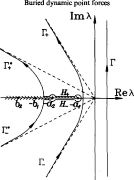
t2 --a: sine,, *: where (40)Fig. 2. Deformed integral contour as presented in (39), (43), (47) and (SO).
r:
=(y-h)2+X2, cose2 = ;, sine, = y-h.r2
This represents essentially a transformation from the f-plane to the I-plane which
changes the path of integration I to I*. In the L-plane, (40) describes a hyperbola as shown
in Fig. 2 (IY,. and r_). When t = alrz = Tpp, the imaginary part of Iz vanishes, and the
vertex of the hyperbola is defined by 1 = -a, cos e2. The parameter t varies from a,r, to cc as 1 moves away from the real axis in either the upper or lower half-plane. Since we are considering the case al < u2, the hyperbola does not intersect any branch cut of the integrand. The hyperbolic paths I+ and I_ are shown in Fig. 2. These paths form a suitable deformed integral contour to replace the original integral path I. The second term of (28) becomes
(41)
where 2, = lr, (r2, e2, t) in (40). From (38), the inversion of the Laplace transform in the time domain is
(42)
The wave front arrives at the time t = Tpp, with the subscript PP denoting the longitudinal
wave reflected from the interface by the incident longitudinal wave.
As the Cagniardde Hoop method is employed on the third term of (28), let
-cqy+j31h-lx = t. (43)
From the formulation of a quartic algebraic equation, the roots can be obtained explicitly and are presented in the Appendix. When the imaginary part of 1 vanishes, the cor-
responding time t is denoted by Tsp. As t extends from Tsp to co, the integral path extends
from a curve and approaches a straight line. The intersection with the real axis is always located between the branch points -a, and ul. The third term of (28) then becomes
4520 Chien-Ching Ma and Kuo-Cheng Huang
The inversion of the Laplace transform is
(45)
where & is the root of (43) and Tsp denotes the time at which the reflected longitudinal wave front generated by the incident shear wave arrives. a&/at can be obtained by taking a derivative of (43), which yields
A similar procedure is applied to the fifth term of (28), let
-/3,y+a*h-ax = t.
Following the same argument as described from (43) to (46), it becomes
where & is the root of (47), and
(46)
(47)
(48)
(49)
TPS denotes the time at which the reflected shear wave induced by the incident longitudinal wave arrives. The deformed integral path is similar to the paths r+ and l?_ represented in Fig. 2. The intersection of the deformed path with the real axis is always located in the region between --al and a,.
Now let us consider the sixth term of (28). When we let
-fi,(y-@-Ix = t,
(50)
(50) can be solved for 1 explicitly to yield
arg(r2,e2,t) =
-;cos8,*iJ--
--b: t2 sine,.rS (51)
When t = blr2, it indicates the time at which the reflected shear wave front generated by the incident shear wave arrives and is denoted by Tsp The deformed integral contour (r*, and I?) is-shown in Fig. 2. If bl 1 cos& 1 r al, an additional integral path from t = THD to
t = Tss which embraces the branch cut must be considered. In this integral interval, 1 is
for THD < t -c T,,, (52) where
THD = -,/m(y-h)fa,x. (53)
This additional integral path represents the head wave induced by the incident shear wave,
where the wame front of the head wave arrives at time t = TED. The final form of the sixth
term of (28) in time domain becomes
~,,~(~,y,t) =:Im R“6(&)s H(t-T&+:Im
[ at] (54)
where il, = &(rz, &, t) in (51) and A7 = &+(rZ, &, t) in (52).
The inverse Laplace transform of the refracted part in the upper medium of solid 2 for y 2 0 can be evaluated in the same manner as we have discussed for solid 1 previously. The four refracted waves induced are the refracted longitudinal wave induced by the incident longitudinal wave (P/P wave), the refracted shear wave induced by the incident longitudinal wave (P/S wme), the refracted longitudinal wave induced by the incident shear wave (S/P wave) and the refracted shear wave induced by the incident shear wave (S/S wave). We introduce Cagniard contours by setting
P/P wave : a2y+alh-Ax = t, (55)
S/P wave : a,y+P,h--3ix = t, (56)
P/Swave: B2y+a,h-Ax = t, (57)
SISwave: j?zy+jllh-Ix = t. (58)
The roots for 1 in (55)-(58) can be obtained explicitly from the formulation of a quartic algebraic equation which is presented in the Appendix. When the imaginary part of the roots in (55)-(58) vanishes, the correspondent time is denoted by Tpip, TsIp, Tpis and
Tsls, respectively. The refracted wave fronts for P/P, S/P, P/s and S/S wave will arrive at
the time Tplp, TsIp, Tpis and Tsis, respectively. The wave fronts for refracted waves are not radially symmetric waves. For the case we consider, i.e. al < a2 < b, < b2, the vertices of curves presented by (55) and (57) are always located on the real axis between the branch points at ---zl and a,. However, the vertices of curves presented by (56) and (58) may intersect the branch cut, which will induce head waves. Qualitative diagrams of the wave fronts for the three different cases are given in Figs 3a-c. In these diagrams, the ratio of the wave speed is set to be 5 : 4 : 3 : 2. The transient solutions for refracted waves in time domain are
SIP wave : aYY2(x,y,t) = ~Im[FWZ9~~(t-TT,d,
P/S wave : oyy2(x,y,t) =~Irn[F:(nl)~~(t-T~,~),
(59)
4522 Chien-Ching Ma and Kuo-Cheng Huang Case 1 : b, > a, > b, > a, (a) (b) 2 T Case 2: 4 > b, b a2 > a, Case 3 : 6, > b2 > a2 > a,
Fig. 3. (a) Wave fronts of the incident, reflected and refracted waves for a, < b, < a2 -c b2. (b) Wave fronts of the incident, reflected and refracted waves for a, < a2 < b, < b2. (c) Wave fronts of the
incident, reflected and refracted waves for a, < Q < b2 < b,.
(62)
The values of ,?j’, L,*, A: and A$exact transient solutions for stresses solid 2 are summarized as follows
are the roots of (55)-(58), respectively. Finally, the
ayu, CXXY cXY and displacements u,,, U, in solid 1 and
CT~,,, (x, y, t) = : ,& Im
I
[ 1
Fj(L,) 2 H(t - Ti) + Head waves, (63)a,,2 (x9 Y, 0 =:,$Irn[FNiR$b-TafHeadwaves, (W
Buried dynamic point forces
H(t-T,)dt+Headwaves,
G?(Q) 2
1
H(t- Ti*) dt+ Head waves,ox,.1 (x, y, t) = : ,$, Im
[
1
Hi(Li) $$ H(t - rrl,) + Head waves,
eXX2 (x, y, 1) = 4 $, Im H(t - Ti*) + Head waves,
CJ,~~ (x, y, t) = z ,i Im
1-l [
1
Ji(ni) 2 H(t - Ti) + Head waves,
oXY2 (x, y, t) = : $‘, Im
[
1
Jj+Q,*) $ H(t - Ti*) + Head waves,
H(t- 5“)) dt+Head waves,
G(&t)$
1
iY(t-mdt+Head waves.(65)
(66)
(67)w-9
(69) (70) (71) (72)The functions Fiy F?, Gi, G,!: Hi, Hf, Ji, JT, Ki and e are expressed in the previous section. The number Iof solutions for head waves in (63)-(72) depends on the relative magnitudes of the slownesses, and three cases are completely presented in Figs 3a-c.
STATIC SOLUTIONS
One of the well known 3-D static solutions is Mindlin’s solution (1936) for a point force in the interior of an elastic half-space. The solution of the stress distribution to the equivalent 2-D problem was given by Melan (1932) and the displacement was obtained by Telles and Brebbia (1981) by integrating Mindlin’s expressions with reference to the out- of-plane coordinate of the load point. Melan’s solution is a particular case of the more general solutiSon for bimaterial interface problem presented in this section. The special case of a bonded interface where the second material is rigid, i.e., an elastic half-space with a ftxed boundary, has been solved by Phan-Thien (1983). The static solution of cryu for applying a static vertical point force in the interior of an elastic bimaterial medium can be obtained from the transient solutions expressed in the previous section by assuming that
the time t approaches infinity, which is equivalent to letting the variables Ai and &+ tend to
infinity in (63) and (64). Avoiding the tedium of algebraic calculations, only the final expressions are provided. The static solution of stress c,,~ in the lower half plane (solid 1) written in the form of slownesses is
r$,, (x, y) =
5
[
Y+hn
x2+(y+h)2+
4 -b:
[X2-(y+h)2](y+h) b:[x2 + (.Y+h)‘]*
4(1-y)(a:-b:)2yh(y-h)[(3x2-(y-h)2] - b:[(l-y)(a:+b:)-2b:][x2+(y-h)2]34524
where
Chien-Ching Ma and Kuo-Cheng Huang
+
(1-y)(b:--a:)[(a:+b:)y+(a:-b:)hl[x2-(y-h)21
b:[(l-Y)(a:+b:)-2b:][x2+(y-h)Z]2 {(a:+b:>(b:-a:)+Y2(a:+b:)(u:-b:)}(y-h)
-[(1-Y)(u:+b:)+2Yb:1[(1-Y)(u:+b:)-2b:][x~+(y-h)~]
1
’ (73)The first two terms of (73) come from the contribution for incident P and S waves,
while the last three terms come from the contribution of reflected PP, PS, SP and SS
waves. The static solution in the upper half plane (solid 2) is
$Jx, y) = a0 [
-2(Y’(u:+b:)(b~-e:)+Y(b:b:+u:a:)} Y+h
71 [(1-Y)(a:+b:)-2b:][(1-Y)(u:+b:)+2Yb:] xZ+(y+h)2
2(u: - b:)yh 2(G - a:)Yy X2-(y+h)2
-
[(l-Y)(a:+b:)--2bT] + [(l-Y)(a:+b:)+2Yb:] [X2+(y+h)2]2
1
.
(74)If the above mentioned static solutions are written in the form of the Poisson’s ratio, which is more convenient in practical application, the results are
GA(X?Y) =: [ x2+y(;;@2 - 2(l;vl) (y;;y(;y;);;)2] 2(1-Y) + (1 --v,)]l +Y(3-4%)1 yh(y--N3x2 - (y-N21 [x2 + (y-h)2]3 (1-Y) ](3-4v,)y-~l]x2-(y-Wl
- 2(1 -vi)[l +Y(3-4v,)] [x2 +(y-h)2]2
3(1 -y2)+4(y2v1 -v2) (y-h)
+ (3-4v,+~)[l+Y(3-4v,)l ~~+(y-h)~
1
’
(75)d (x
v)
= 2
2(Y2(3-4v1)+Y[5-6(v, +v2)+W21} y+hYY2 ’ n
[ (Y+3-4v,)]l+Y(3-4v,)l x2+(y+h)2
2YY 2Yh X2--(y+h)2
-
i Y+3-4”~ + l+Y(3--4~1) 1 [~‘+(y+h)~]~
1
’
(76)Some special cases can be used to check the results presented in (75) and (76). The stress ayu should be continuous along the interface, which can be examined be taking y = 0 in (75) and (76). The solution for a point body force in a homogeneous medium can be obtained by setting y = 1 and v1 = v2 = Y in (75) or (76). Finally, the solution for a point force in the interior of an elastic half-space can be derived from (75) and (76) by setting y = 0 and the well known Melan’s solution is obtained.
The correspondent static solutions for the stress cXX and the displacements U, and z+
a’,1 (x:, y) = 2 [
2 y+h
1 (y+h)[x2
-(Y+h)21
71 ~--VI
x2+(y+h)2 +2(1--v,) [x’+(y+h)2]2w -4 yh(y-h)Px2 -
b+-h)2l
- Cl--v,w
+Y(3-4vdl [x2 + (y-h)2]3 (1-Y)+ 2(1-v,)[l
+y(3-4v,)l[(3-4v,)y--l[x2-(y--h)21
[x2 -t(y-h)2]2 + (3-4v2)(2--3v,)-(3-4v1)[2y(l-&)+y2v,] y-h(1 -h)(Y+3-‘b)[l +Y(3-4”,)1 x2+(y-h)’
1
’
a’
tx
yj
= cp
2(y2(3-4v,)+~[(l -h)(--3+2vz)+‘b(l -VI)]) y+hxx2 3 5T (11’+3-4~,)[1+~(3-4~,)1 x2+(y+h)2 + 2YY 2yh y+3--4% + l+y(3-4v1) x2-(y+h)2 [x2+(y+h)2]”
1
’
+ 4(l -y)xyh(y-h) 1 [1+~(3-4v,)1 [x’+(y-h)‘]* (I-y)(3--4~1) x(y+h) - [l+y(3-4v,)1 x2+(y-h)2 - (1-2~,)(3--‘h)-~(l-2v,)(3-4v,)~~~. (~+3-4v,)[l+y(3-4~,)1 YYyh
Xy+3-4% + l+Y(3-4v1) 1 x2+(y+h)2
Y(1 -Y)(3-4vd(l-2vJ
+ (y+3-4v,)[l +y(3-4v,)] tan-’ y;Th ’
u’,l(X,Y) = - Co Tln[x”+(y+h)“]+ X2 4(1--v,)p,n x2f(y+h)’ 4( 1
-
y)x2yh 1 - l+~(3--4v,) [x2+(y-h)2]2 + (l-y)[(3-4v,)x2+2yh] 1 1 +y(3 -4v1) x’+(y-h)’ (77) (78) (79 (80) +(3 -4%) [8(1
-v,)2-(3-4v~)]-(3-4v,)y[(3-4v~)y+2(1-2v~)(1-2v2)] 2(y+3-4v,)[l+y(3-4vJ x In [x2 +(y-h)21 ,(81)
+ yx2+yh(y+h)
y+3-h2 - 1:~~~~~,)],z+(:+h)2}’ (82)4526 Chien-Ching Ma and Kuo-Cheng Huang NUMERICAL RESULTS
We have obtained explicit transient and static solutions for stresses and displacements
in previous sections. We would like to investigate the transient response of stress eYY for the
cases a, < bl < a2 < b2 (case 1) and a, -C a2 < b, < b2 (case 2). We consider the point dynamic force applied suddenly at the point (0, -h) in the y direction, i.e. 6 = 0” and T,(I) = T2(A) = 1, the induced wave fronts of incident, reflected and refracted waves are shown in Figs 3a and 3b. The wave fronts of P, S and PP, SS are circular curves, the HD wave is an inclined straight line, PS, SP, P/P, P/S, S/P and S/S wave fronts are smooth
curves which are constructed by numerical calculations. For the first case (case 1,
al c b, c a2 < b2), the following ratios of slownesses are used, a, : b, : a2 : b2 = 2 : 3 : 4 : 5
(y = p2/p, = 0.3 or y = p2/p, = 0.5). The field points selected for calculation are
(OS/r, -0.5/z) and (0, -0.5h) in solid 1, (0.5/r, 0) and (h, 0) on the interface, (0.5/r, 0.5h) and
(0,0.5h) in solid 2. The transient response of crYv are presented in Figs 46, respectively. For
the second case (case 2, al < a2 < b, c b2 and a, : a2 : b, : b, = 2 : 3 : 4 : 5, y = p2/p, = 0.3),
the dimensionless transient stress haJo, as function of the dimensionless parameter t/qh
for the field points in solid 1, in the interface and in solid 2 is shown in Figs 7-9, respectively. In these figures, the stress fields behave with a square root singularity at the wave front, except in the case of the head wave. The arrival times of all the incident, reflected and refracted wave fronts are also indicated in the figures. The corresponding static values are also shown in these figures. The transient solutions are shown to approach the static solution as time increases. Generally speaking, the dynamic transient effect is important under dynamic loading conditions. In the transient period, the tensile or compressive effect will change radically when the reflected wave arrives.
Fig. 4. Transient normal stress oz of points in solid 1 for a, < b, -c a2 < b2.
2.2 ; ~/@,=0.9 (case I) ‘-l ----z/h=.0 &‘A=-.5 1.7 -z/h=O.S.y/h=-.5 y ,.2 :, 1!:%>...* PP sp b’ I. & 0.7 _ _ _ _ { _.__..~_ : _:‘_~~-_===-_-_-_-_-=. 0.2 I I P -8 PP ’ BP ’ I ps as -0.3 (11111111,(,,,,,,,,,,,,,,,,,,,(,,,,,~ 0.4 0.9 t/a’;x 1.9 b” \ 0.5 bp we 0.3
Q.7 11
Fig. 6. Transient normal stress az2 of points in solid 2 for a, < b, < a2 < bP
Fig. 7. Transient normal stress uz2 of points in solid 1 for a, < a2 < b, < b2.
-0.11.,,,..,..,..,,,,,,,,..,,,,,..,.,,.
1.0 2.0
t/a:%
4.0
Fig. 8. Transient normal stress az2 of points in the interface for a, < aZ < b, < bl.
CONCLUSIONS
In this study, the transient solutions of stresses and displacements by applying a dynamic point force in the interior of a bimaterial medium with perfect bonding at the
interface are studied in detail. The Cagniardde Hoop inverse method is used, enabling us
to investigate :in detail the structure of the wave pattern. It is worth noting that the static solution for a point force in the interior of a bimaterial medium can be obtained from the
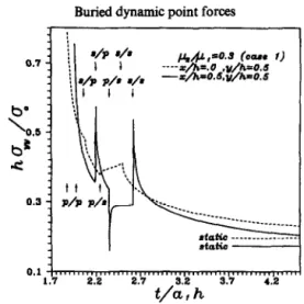
4528 Chien-Ching Ma and Kuo-Cheng Huang 0.6 /1c1&,=0.3 (care 2) ----z/h=O. ,y/h=O.S --z/h-O.&y/h=O.S t/a,h
Fig. 9. Transient normal stress u22 of points in solid 2 for a, -z a* < b, < b,.
transient solution by taking the appropriate limit. As far as the authors know, this complete
formulation for static solution has never been presented previously, although it is of
fundamental importance for problems concerning a bimaterial interface. The fundamental solutions of transient and static problems for a point load within the bimaterial interface presented in this study will be very useful for the application to the boundary element method. The present method provided in this study has alreidy been extended to solve the more difficult problem of transient wave propagation in layered medium with finite dimension. The results will be shown in a future paper.
To investigate the characteristic time after which the transient effect can be neglected, numerical results of stress based on the transient analysis are presented and compared to the corresponding static values. It is found that the dynamic transient solution approaches the static value very quickly after the last wave (SS wave in solid 1 and S/S wave in solid 2) has passed the field point.
Acknowledgements-The financial support of the authors by the National Science Council, Republic of China,
through Grant NSC 81-0422-E002-557, is gratefully acknowledged.
REFERENCES
de Hoop, A. T. (1958). Representation theorems for the displacement in an elastic solid and their application to elastodynamic diffraction theory. Ph.D. thesis, Technische Hogeschool, Deft, Netherlands.
Gakenheimer, D. C. and Miklowitz, J. (1969). Transient excitation of an elastic half space by a point load travelling on the surface. ASME J. Appl. Mech. 36, 505-515.
Garvin, W. W. (1956). Exact transient solution of the buried line source problem. Proc. Royal Sot. (London)
A234,528-541.
Lamb, H. (1904). On the propagation of tremors over the surface of an elastic solid. Phil. Trans. Royal Sot.
(London) A203, l-42.
Lapwood, E. R. (1949). The disturbance due to a line source in a semi-infinite elastic medium. Phil. Trans. Royal
Sot. (London) AZ42,63-100.
Melan, E. (1932). Der spannungszustand der durch eine einzelkraft in innem beanspruchten halbscheibe. 2.
Angew. Math. Mech. 12,343-346.
Mindlin, R. D. (1936). Force at a point in the interior of a semi-infinite solid. Physics 7, 195-202.
Nakaguma, R. K. (1979). Three dimensional elastostatics using the boundary element method. Ph.D. thesis, University of Southampton, UK.
Nakano, H. (1925). On Rayleigh waves. Jap. J. Astr. Geophys. 2,233-326.
Payton, R. G. (1967). Transient motion of an elastic half-space due to a moving surface line load. Znt. J. Engng
Sci. 5,49-79.
Payton, R. G. (1968). Epicenter motion of an elastic half-space due to buried stationary and moving line sources.
Znt. J. Solids Structures 4,287-300.
Pekeris, C. L. (1955a). The seismic surface pulse. Proc. Nut. Academic Sot. 41,469-480. Pekeris, C. L. (1955b). The seismic buried pulse. Proc. Nat. Academic Sot. 41.629-638.
Pekeris, C. L. and L&on, H. (1957). Mot& of the surface of a uniform elastic half-space produced by a buried pulse. J. Acoustical Sot. of America 29,12331238.
Phan-Thien, N. (1983). On the image system for the Kelvin-states. J. Elasticity 14,231-235.
Telles, J. C. F. and Brebbia, C. A. (1981). Boundary element solution for half-plane problems. Znf. % Solidr
Tsai, C. H. and Ma, C. C. (1991). Exact transient solutions of buried dynamic point forces and displacement jumps for an (elastic half space. Zni. J. Solids Structures 28,955-974.
APPENDIX
The idea of the Cagniard-de Hoop method is to deform the path of integration in the I-plane in such a manner that the inverse Laplace transform of the integral along the new path of integration can be obtained by inspection. The desired path of integration in the I-plane discussed in this manuscript for SP wave (eqn (43)), PS wave (eqn 47)), P/P wave (eqn (55)), S/P wave (eqn (56)) P/S wave (eqn (57)) S/S wave (eqn (58)) can be expressed by the following equation
+myy+J-lx = t, (Al)
where p and 4 are constants and p = a,, q = b, for SP wave, p = b,, q = ai for PS wave, p = a2, q = a, for PIP wave, p = 4, q := b, for S/P wave, p = b,, q = a, for P/S wave, p = bZ, q = b, for S/S wave.
Equation (Al) can be rewritten to the following quartic equation for 1
where ~4+z,~~+zz)**+zj~+z4 = 0, (A2) I, = 2(x2 +y* +h*)(t* -p2y2 -q*h*) (x’+y’+h*)*-4y2h2 ’ z =4x2t2+4y2hZ@2+q2)+2(~2+yZ+h2)(t2-p2y2-q2h~) 2 (xz+y2 +h*)* -4y2h2 z 4 = (t2 -p2y2 -q2h2) -4yzh2p2q2 (x2+y2+hZ)Z-4yZh2
The quartic eqn (A2) can be solved and the analytical solutions for proper roots are expressed explicitly as follows where A,* = ;[N+ Iv-2(Uf~s?4)], N = -;[Z, -d-q, U = S+ TfZ,/3, s=sJkJFzF, T= ‘Jm, w=&[-9Z2(Z,Z,-4Z,)-27(4Z,Z,-Z:-Z;Z,)+2Z;], v= ~[3(z,z,-4z,)-z:].