A note on a polynomial time approximation scheme
for the MRCT problem
Bang Ye Wu Kun–Mao Chao
April 1, 2004
1
Further improvement
Let S be a minimal δ-separator of T . The strategy of algorithms shownb
in our previous note on 3/2-approximation is to “guess” the structure of S and to construct a general star with the guessed structure as the core. If
T ∈star(S), by the lemmas in the previous note, C(T ) ≤ 2n X v∈V (G) dG(v, S) + (n2/2)w(S), and C(T ) ≥ 2(1 − δ)nb X v∈V dTb(v, S) + 2δ(1 − δ)n2w(S).
The approximation ratio, by comparing the two inequalities, is max{ 1
1 − δ, 1 4δ(1 − δ)}.
The ratio achieves its minimum when the two terms coincide, i.e., δ = 1/4, and the minimum ratio is 4/3. In fact, by using a general star and a (1/4)-separator, it is possible to approximate an MRCT with ratio (4/3) + ε for any constant ε > 0 in polynomial time. The additional error ε is due to the difference between the guessed and the true separators.
By this strategy, the approximation ratio is limited even if S was known exactly. The limit of the approximation ratio may be mostly due to that we consider only general stars. In a general star, the vertices are always connected to their closest vertices of the core. In extreme cases, roughly half of the vertices connected are to both sides of a costly edge. This results in the cost (n2/2)w(S) in the upper bound of a general star. To make a
breakthrough, the restriction that each vertex is connected to the closest vertex of the core needs to be relaxed.
A metric graph is a complete graph with triangle inequality, i.e., each edge is a shortest path of its two endpoints. If the input graph is a metric graph, the core will be a two-edge path, and each vertex is adjacent to one of the “critical vertices”— a centroid and the two endpoints of a path separator. Define k-stars to be the trees with at most k internal vertices. The constructed approximation solution is a 3-star. More importantly, k-stars have no such restriction like general stars and can be used to approximate an MRCT more precisely. Later in this chapter we shall see how it works.
However, k-stars work only for metric graphs. The class of metric graphs is an important subclass of graphs. Solving the MRCT problem on metric graphs is itself meaningful. Before considering the approximation problem on metric graphs, two questions come to our minds:
• What is the computational complexity of the MRCT problem on
met-ric graphs, NP-hard or polynomial-time solvable?
• If it is NP-hard, does its approximability differ from that of the general
problem?
We shall answer the questions in the next section.
2
A Reduction to the Metric Case
In this section, we shall show that the MRCT problem on general inputs can be reduced to the same problem with metric inputs. The reduction is done by a transformation algorithm.
Definition 1: The metric closure of a graph G = (V, E, w) is the complete graph ¯G = (V, V × V, ¯w) in which ¯w(u, v) = dG(u, v) for all u, v ∈ V .
Let G = (V, E, w) and ¯G = (V, V × V, ¯w) be its metric closure. Any
edge (a, b) in ¯G is called a bad edge if (a, b) /∈ E or w(a, b) > ¯w(a, b).
For any bad edge e = (a, b), there must exist a path P = SPG(a, b) 6= e
such that w(P ) = ¯w(a, b). Given any spanning tree T of ¯G, the algorithm
can construct another spanning tree Y without any bad edge such that
C(Y ) ≤ C(T ). Since Y has no bad edge, ¯w(e) = w(e) for all e ∈ E(Y ), and Y can be thought of as a spanning tree of G with the same routing cost.
Algorithm: Remove bad Input: A spanning tree T of ¯G.
Output: A spanning tree Y of G such that C(Y ) ≤ C(T ). Compute all-pairs shortest paths of G.
(I) while there exists a bad edge in T Pick a bad edge (a, b). Root T at a.
/* assume SPG(a, b) = (a, x, ..., b) and y is the parent of x */ if b is not an ancestor of x then
Y∗← T ∪ (x, b) − (a, b);Y∗∗← Y∗∪ {(a, x)} − {(x, y)};
else
Y∗← T ∪ (a, x) − (a, b);Y∗∗← Y∗∪ {(b, x)} − {(x, y)};
if C(Y∗) < C(Y∗∗) then Y ← Y∗ else Y ← Y∗∗
(II) T ← Y
The algorithm computes Y by iteratively replacing the bad edges until there is no bad edge. It will be shown that the cost is never increased at each iteration and it takes no more than O(n2) iterations. We assume that the shortest paths obtained in the first step have the following property: If
SPG(a, b) = (a, x, . . . , b), then SPG(a, b) = (a, x) ∪ SPG(x, b). This assump-tion is not strong since almost all popular algorithms for all-pairs shortest paths output such a solution.
Proposition 1: The while loop in Algorithm Remove bad is executed at most O(n2) times.
Proof: For each bad edge e = (a, b), let h(e) be the number of edges in
SPG(a, b) and f (T ) =Pbad eh(e). Since h(e) ≤ n − 1, f (T ) < n2 initially.
Since (a, x) is not a bad edge, it is easy to check that f (T ) decreases by at least 1 at each iteration.
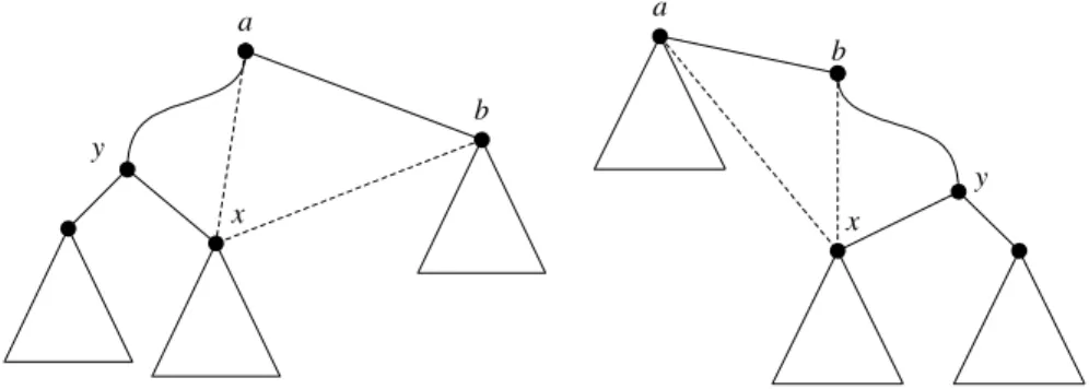
Proposition 2: Before instruction (II) is executed, C(Y ) ≤ C(T ). Proof: For any node v, let Sv = V (Tv). As shown in Figure 1, there are
two cases. Case 2 is identical to Case 1 if the tree is re-rooted at b and the roles of a and b are exchanged. Therefore, only the inequality for Case 1 needs to be proved, i.e., x ∈ Sa− Sb.
If C(Y∗) ≤ C(T ), the result follows. Otherwise, let U
1 = Sa− Sb and
a b y x a b y x
Figure 1: Remove bad edge (a, b). Case 1 (left) and Case 2 (right).
both in U1 (or both in Sb), we have
C(T ) < C(Y∗) ⇒ X u∈U1 X v∈Sb dT(u, v) < X u∈U1 X v∈Sb dY∗(u, v).
Since for all u ∈ U1 and v ∈ Sb, dT(u, v) = dT(u, a) + ¯w(a, b) + dT(b, v)
and dY∗(u, v) = dT(u, x) + ¯w(x, b) + dT(b, v),
X u∈U1 X v∈Sb (dT(u, a) + ¯w(a, b) + dT(b, v)) < X u∈U1 X v∈Sb (dT(u, x) + ¯w(x, b) + dT(b, v)) ⇒ |Sb| X u∈U1 dT(u, a) + |U1||Sb| ¯w(a, b) < |Sb| X u∈U1 dT(u, x) + |U1||Sb| ¯w(x, b) ⇒ X u∈U1 dT(u, a) + |U1| ¯w(a, b) < X u∈U1 dT(u, x) + |U1| ¯w(x, b).
Note that Sb6= ∅ since the inequality holds. By the definition of the metric
closure, ¯w(a, b) = ¯w(a, x) + ¯w(x, b), and then
X
u∈U1
Now consider the cost of Y∗∗. (C(Y∗∗) − C(T )) /2 = X u∈U2 X v∈Sx (dY∗∗(u, v) − dT(u, v)) + X u∈U1 X v∈Sb (dY∗∗(u, v) − dT(u, v)) .
Since dY∗∗(u, v) ≤ dT(u, v) for u ∈ U1 and v ∈ Sb, the second term is not
positive. By observing that dT(u, v) = dT(u, x) + dT(x, v) and dY∗∗(u, v) =
dT(u, a) + ¯w(a, x) + dT(x, v) for any u ∈ U2 and v ∈ Sx, we obtain
(C(Y∗∗) − C(T )) /2
≤ X
u∈U2
X
v∈Sx
(dT(u, a) + ¯w(a, x) − dT(u, x))
= |Sx|
X
u∈U2
(dT(u, a) + ¯w(a, x) − dT(u, x))
= |Sx|
X
u∈U2
(dT(u, a) − dT(u, x)) + |U2||Sx| ¯w(a, x)
≤ |Sx| X
u∈U1
(dT(u, a) − dT(u, x)) + |U2||Sx| ¯w(a, x) (2)
< −|U1||Sx| ¯w(a, x) + |U2||Sx| ¯w(a, x) (3)
≤ 0.
(2) is obtained by observing that U1− U2 = Sx and dT(u, a) > dT(u, x) for
any u ∈ Sx. (3) is derived by applying (1). Therefore, C(Y∗∗) < C(T ) and
the result follows.
The next lemma follows Propositions 1 and 2, and that each iteration can be done in O(n) time.
Lemma 1: For any spanning tree ¯T of ¯G, it can be transformed into a
spanning tree T of G in O(n3) time and C(T ) ≤ C( ¯T ).
The above lemma implies that C(mrct(G))≤ C(mrct( ¯G)). It is easy
to see that C(mrct(G))≥ C(mrct( ¯G)). Therefore, we have the following
corollary.
Corollary 2: C(mrct(G))=C(mrct( ¯G)).
Let ∆MRCT denote the MRCT problem with metric inputs. We have the next theorem.
Theorem 3: If there is a (1+ε)-approximation algorithm for ∆MRCT with time complexity O(f (n)), then there is a (1 + ε)-approximation algorithm for MRCT with time complexity O(f (n) + n3).
Proof: Let G be the input graph for the MRCT problem. The metric closure ¯G can be constructed in time O(n2log n + mn). If there is a (1 +
ε)-approximation algorithm for the ∆MRCT problem, a spanning tree T of ¯G
can be computed in time O(f (n)) such that C(T ) ≤ (1 + ε)C(mrct( ¯G)).
Using Algorithm Remove bad, a spanning tree Y of G can be constructed such that C(Y ) ≤ C(T ) ≤ (1 + ε)C(mrct( ¯G))= (1 + ε)C(mrct(G)). The
overall time complexity is then O(f (n) + n3).
Corollary 4: The ∆MRCT problem is NP-hard.
3
A Polynomial Time Approximation Scheme
3.1 Overview
We sketch a Polynomial Time Approximation Scheme (PTAS) for the MRCT problem in this section.
As described previously, the fact that the costs w may not obey the triangle inequality is irrelevant, since we can simply replace these costs by their metric closure. Therefore, in this section we may assume that G = (V, E, w) is a metric graph.
We use k-stars, i.e., trees with no more than k internal nodes, as a basis of our approximation scheme. In Section ?? we show that for any constant
k, a minimum routing cost k-star can be determined in polynomial time. In
order to show that a k-star achieves a (1 + ε) approximation, we show that, for any tree T and constant δ ≤ 1/2:
1. It is possible to determine a δ-separator, and the separator can be cut into several δ-paths such that the total number of cut nodes and leaves of the separator is at most d2
δe − 3. (Lemma ??)
2. Using the separator, T can be converted into a (d2δe−3)-star X, whose
internal nodes are just those cut nodes and leaves. The routing cost of X satisfies C(X) ≤ (1 +1−δδ )C(T ). (Lemma ??)
By using T =T =mrct(G), δ =b 1+εε and finding the best (d2δe − 3)-star K, we obtain the desired approximation
C(K) ≤ (1 + δ
Before going into the details of the general case, take a look at how to find a 3/2-approximation of an MRCT and its performance analysis.
Recall that a centroid of a tree is the vertex whose removal cuts the tree into components of no more than n/2 vertices. Let T be an MRCTb
of a metric graph G. Root T at its centroid r. For an edge (u, v) withb
parent v, the routing load of the edge is 2x(n − x), in which x is the number of descendants of u. (For convenience, we assume that a vertex is also a descendant of itself.) For a desired positive δ ≤ 1/2, removing all vertices with number of descendants no more than δn, we may obtain a connected subgraph S of T . The subgraph S is a minimal δ-separator. In the case that
δ = 0.5, S contains only the centroid. If the δ-separator S of the MRCT is
given and, for each vertex not in S, its lowest ancestor in S is also known, we may easily construct a 1/(1 − δ)-approximation Y of the MRCT as follows:
• S ⊂ Y .
• For each vertex u not in S, connect it to its lowest ancestor v in S by
adding edge (u, v).
The approximation ratio of Y can be shown by the following two obser-vations.
• For each edge in S, the routing load in Y is the same as that in T .b • For each edge (u, v) not in S, the routing load in Y is 2(n−1). However,
there is a path from u to v inT of which each edge has routing loadb
no less than 2(1 − δ)n, and the length of the path is at least the same as the edge (u, v).
For example, consider the simplest case that δ = 1/2. A 1/2-separator contains only one vertex. Assume that r be such a vertex on an MRCT
b
T . For every other vertex, the ancestor in the separator is r. Connecting
all other nodes to r, we obtain a star Y . The routing cost of Y is the sum of all edges (v, r) multiplied by its routing load 2(n − 1). For each vertex
v, there is a path from v to r in T . Since r is a 1/2-separator ofb T , theb
routing load of the path is at least n and the path is no shorter than the edge (v, r) by the triangle inequality. Consequently Y is a 2-approximation of the MRCTT . Since the separator contains only one vertex, we may tryb
all possible vertices and it leads to an O(n2) time 2-approximation of the
MRCT problem on metric graphs.
But when δ < 1/2, the separator may contain as many as Ω(n) vertices, and it is too costly to enumerate all possible separators. However, instead of
Var r a Va b V r Vb Vbr a r b V ar Vbr a r b V ar Vbr a r b V ar Vbr a r b V ar Vbr
Figure 2: An MRCT and the four 3-stars.
the entire separator, we may achieve the same ratio by knowing only some
critical vertices of the separator. In the following, we shall take δ = 1/3 as
an example to show that we only need to know three critical vertices of the separator to construct a 3/2-approximation.
Root the MRCT T at its centroid r. There are at most two subtreesb
which contain more than n/3 nodes. Let a and b be the lowest vertices with at least n/3 descendants. We ignore the cases where r = a or r = b. For such cases, the ratio can be shown similarly. Let P be the path from a to
b. Obviously the path contains r and is a minimal 1/3-separator. We shall
transform T into a 3-star with internal nodes a, b, and r such that its routing cost is no more than 3/2 of that ofT . As shown in Figure 2, let us partitionb
all the vertices into Va, Vb, Vr, Var, and Vbr. The sets Va, Vb, and Vrcontain
the vertices whose lowest ancestor on P is a, b, and r, respectively. The set
Var (and Vbr) consists of the vertices whose lowest ancestor on P is between
a and r (and between b and r, respectively).
First replace P with edges (a, r) and (b, r). For each vertex v in Va (or
Vb, Vr), edge (v, a) (or (v, b), (v, r) respectively) is added. For the vertices
in Var, we consider two cases. Either all of them are connected to a or all of them are connected to r. The vertices in Vbr are connected similarly. The
four possible 3-stars are illustrated in Figure 2.
Now consider the routing cost ofT . For each vertex v, the routing loadb
of the path from v to P is no less than 4n/3 since P is a 1/3-separator. For each edge e of P , since there are at least n/3 nodes on either side of it, the routing load is no less than 2(n/3)(2n/3) = 4n2/9. Therefore we have the
following lower bound of the routing cost of the MRCT:
C(T ) ≥ (4n/3)b X
v
In either of the 3-stars constructed above, for each vertex v in Va∪Vr∪Vb,
the routing load of the edge incident to v is 2(n − 1), and the edge length is at most the same as the path from v to P on T . For each node v in Var, by
the triangle inequality, we have
(w(v, a) + w(v, r))/2 ≤ dTb(v, P ) + dTb(a, r)/2.
Note that there are no more than n/6 nodes in Var. For edge (a, r), the
routing load is no more than 2(n/2)(n/2) = n2/2. (Note: For this simple
case that δ = 1/3, this bound is enough. However, a more precise analysis of the incremental routing load is required for smaller δ.)
For the nodes in Vbr, we may obtain a similar result. In summary, the minimum routing cost of the constructed 3-stars is no more than
2(n − 1)X v dTb(v, P ) + (n2/6)(dTb(a, r) + dTb(b, r)) + (1/2)n2w(P ) ≤ 2nX v dTb(v, P ) + (2/3)n2w(P ).
The approximation ratio, by comparing with the lower bound of the optimal, is 3/2.
The method can be extended to any δ ≤ 0.5. Let S be a δ-separator of T . The critical vertex set, defined as the cut and leaf set in the next section, to construct a 1/(1 − δ)-approximation k-star consists of the following vertices.
• The leaves of S as a and b in the above example. • The vertices with more than two neighbors on S.
• Some additional vertices such that all the critical vertices cut the
sepa-rator into edge-disjoint paths and the number of vertices whose lowest ancestors on S belong to the same path is no more than δn/2. Such a path is defined as a δ-path in the next section. In the above example,
r is such a vertex. The vertices a, b and r cut the separator into two
paths, and the number of vertices in either Var or Vbr is no more than
n/6.
We shall show that the number of the necessary critical vertices is at most 2/δ − 3 for any δ ≤ 0.5. Consequently there exists a (2/δ − 3)-star which is an approximation of an MRCT with ratio 1/(1 − δ). The PTAS is to construct the (2/δ − 3)-star of minimum routing cost.
The core of a tree is the subgraph obtained by removing all its leaves. The core of a k-star contains no more than k vertices and therefore the
number of all possible cores is polynomial to k. For each possible core, the algorithm finds the best way to connect the leaves to one of the vertices of the core. A k-component integer vector (n1, n2, . . . , nk) is used to indicate
how many leaves will be connected to each of the k vertices of the core, in which Pini = n − k. There are O(nk−1) such vectors. For each core and
each vector, the routing load on each core edge is fixed since the number of vertices on both sides of the edge are specified by the core and the vector. Therefore the best leaf connection is determined by the leaf edges subject to the numbers of leaves to be connected to the vertices of the core. Such a problem can be solved by solving an assignment problem in O(n3) time.
Consequently the minimum routing cost k-star can be constructed in time polynomial to k and n.
Consider an example for k = 3. For a 3-star, the core is a 3-vertex path. There are O(n3) possible cores. For each possible core (a, b, c), use a
three-component integer vector (x, y, z) to indicate how many leaves will be connected to a, b, and c, in which x+y+z = n−3 and x, y, z are nonnegative integers. There are O(n2) such vectors. For a specified core and a specified
vector, the routing load on each core edge is also fixed. That is, the routing load on (a, b) is 2(x + 1)(n − x − 1) and on (b, c) is 2(z + 1)(n − z − 1). Therefore the best leaf connection is determined by the leaf edges subject to the numbers of leaves to be connected to a, b, c. Such a problem can be solved by solving an assignment problem in O(n3) time. The total time
complexity is O(n2k+2), which is polynomial for constant k. In fact we need
not solve the individual assignment problem for the best leaf connection of each vector. The best leaf connection of one vector can be found from that of another vector by solving a shortest path problem if the two vectors are adjacent. Two vectors are adjacent if one can be obtained from the other by increasing a component by one and decreasing a component by one, e.g., (5, 4, 2) and (5, 3, 3). With this result, the time complexity is reduced to