A three-phase parallel algorithm for solving linear recurrences

(1)

A T H R E E - P H A S E P A R A L L E L A L G O R I T H M F O R S O L V I N G

L I N E A R R E C U R R E N C E S

Kuo-LIANG CHUNG

Department of Computer Science and Information Engineering, National Talwan University, Talpei, Talwan 10764, R. O. C.

F E R N G - C H I N G LIN

Department of Computer Science and Information Engineering, National Taiwan University, Talpei, Talwan 10764, 1t. O. C.

Y E O N G - N A N Y E H

Institute of Mathematics, Academia Sinica, Talpei, Talwan 11529, R. O. C.

(Receieed Me, y, 1990)

A b s t r a c t - - W e present in this paper a three-phase parallel algorithm on the unshtflRe network for solving linear recurrences. Through a detailed analysis on the special nmtrix multiplications involved in the computation we show that the first n terms of an ruth order linear recurrence can be computed in O(m 3 l o g ~ ) time - l i n g O ( m - - - l ~ ) processors. For the usual case when m is a small constant, the algorithm achieves cost optinmlity.

1. I N T R O D U C T I O N

Linear recurrences form an important class of computational problems which arise in many different application areas. Some parallel algorithms have been proposed before for solving linear recurrences. Stone and Kogge [5,6] first presented a recursive-doubling method to solve recurrences through a tricky divide-and-conquer reformulation of the recurrences into ones which use two indices. Based on a depth-width tradeoff in overlaid tree structure, Carlson and Sugls [1,2] presented s network containing multiple shuffle-exchange connections to compute the first n terms of a first-order linear recurrence in

O(n/p)

time using O(plogp) processors. Chung, Lin and Chen [3,7] presented a three-phase algorithm on the unshuffle network [8] for solving the first- and second-order linear recurrences, which reduces the O(n) processors used in [8] to O(n/log n) while retaining the time complexity O(log n).

Consider the ruth-order linear recurrence:

xl -" ai,lZi-1 -}- ai,2zi-2 -b • • • + ai,mzi-m + hi. (1.1) Given a~j, bl, 1 < i < n - 1, 1 _< j _< m, and the initial values z0, Z - l , . . . , ~i-m, we want to compute all the values z~, 1 < i < n - 1. For ease of exposition, we assume t h a t n is a power of 2, n > m, and

n/m

is also a power of 2.

The recurrence in (1.1) can be converted into a first-order recurrence with the aid of companion matrices. Let Zi = [ x i , . . . , z i - m + l , 1] t and

=

l ai,1 ai,2 • •. ai,m-1 ai,m

i 0 ... O O

I . . . 0 0 • . o " o 0 . . . I 0 0 . . . O 0 bi

0

0 O

1 Typeset by . A / ~ - ~ X 187

(2)

which is an (re+l) x (re+l) matrix. W e m a y write (I.I) as Zi =

KiZ~-I.

Given Z0 and Ki, 1 _< i _< n, the problem becomes to compute Zi, I < i < n - 1, because zi equals the first component of

Zi. That is, our task is to compute all the prefix products of Z,-I (=

Kn-IK,~-2... KIZo).

Note

that it takes O ( m n ) time to compute all

Zi

sequentially because the companion matrix-vector

multiplication ( C M - V )

KiZi-1

can be completed in

O(m)

time, due to the special structure of

the companion matrix Ki.

W h e n parallel processing is involved, this good computation property of C M - V s disappears.

In the past, the complexity analysis was oversimplified by considering a matrix-matrix or matrix-

vector multiplication as a one-time step and the parameter m was ignored [5,6]. Based on the

three-phase algorithm on unshufiie networks [3,7], we present in this paper a parallel algorithm

for solving general linear recurrences. W e shall show sharper complexity results in terms of the three parameters n, m and the number of processors used. The performance of a parallel algorithm can be measured by Cost = N u m b e r of Processors x Execution Time. The m i n i m u m cost achievable by our algorithm is O(m2n) with O(m s log ~ ) execution time and O ( m - - i ~ ) processors. Usually, m is a small constant in applications. In such a case, our algorithm achieves optimal cost (')(n) with O(log n) time and (')(n/log n) processors.

2. T H E U N S H U F F L E N E T W O R K

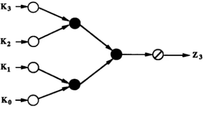
Due to the associativity of multiplication, the three multiplications in Za - KaK2KIKo, where

K0 - Z0, can be performed in any order. Fig. 2.1 shows a possible computation tree for Za. The white nodes in the leftmost stage 0 are used for preparing input data only. The black nodes in stages 1 and 2 perform the multiplication.

K3

K2

KI

K0

Figure 2.1. A computation tree of Zs.

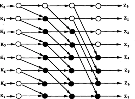
If we combine the computation trees for Zi, 0 < i < 7, an overlaid tree network, as shown in Fig. 2.2, is obtained for computing all the prefix products of Zz. For general n, there are log n + 1 stages of nodes in the network. If each node is implemented by a processor, the number of processors is as large as n(log n + 1), which is going to be reduced to O ( m - - I ~ ) later.

The multi-stage unshufl]e network which can be used to simulate the overlaid tree network is depicted in Fig. 2.3, where Si,j and Pij, 0 < i < n - 1, 1 ~ j _< logn, are simple devices and

processors respectively. Let

qoql

... qa-x (l = log n) be the binary representation of i. The output

line of Pij is connected to Sv_lq0el...q,_2j+t to provide the unshui~e data routing mechanism.

The simple device Sij is capable of producing two copies of its input and sending them to Pid and

Pi+ij except that the bottom

Sn-tj

has only one receiver

P,-t,j.

For tracing the data passing

in the network, each simple device is labelled by a number inside the parentheses to indicate where its data originate. The function of white nodes in a stage of Fig. 2.2 can be controlled by a proper masking mechanism in Fig. 2.3. For example, P0,1 in stage 1, which is masked by a cross mark, merely transmits data to the next stage; P0,2 and P4,2 in stage 2 are masked also. Similarly, in stage 3, P0,s, P2,3, P4,3, P6,3 are masked.

Since the interconnection patterns between the stages of the multi-stage unshuffle network are all identical, we can compress all the stages together to obtain a single-stage unshuffle network as shown in Fig. 2.4, which has only n processors. After each iteration of execution, the processors feed the intermediate results back to the simple devices as inputs for the next iteration. The

(3)

Algorithm for solving linear recurrences

Ko " ~ ~ O ~ Zo

K 4 - - - ~ ~ Z4

Ks-"~ ~

~

Zs

Figure 2.2. Overlaid tree network for computing all prefix values of ZT.

189

Stage 1

Stage 2

Stage 3

Z0 Zx Z2 Z3 Z4 Zs Zs Z7 Figure 2.3. The multi-stage unshuflle network.

masking on the network at different iterations is exactly what we have described for different stages of the multi-stage network.

3. T H E T H R E E - P H A S E A L G O R I T H M

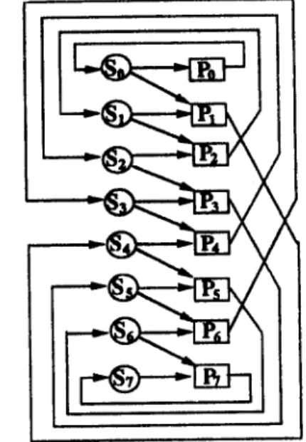
In the following, a modified three-phase algorithm is proposed to reduce the number of processors further. We start with an unshufl]e network of k(<_ n) processors with a bidirectional connection between each pair of Pi and Si. To each processor Pi attach a local memory, which is a linear array of memory blocks C i j , 0 <_ j <_ n / k - 1, as depicted in Fig. 3.1 for n = 8 and k - 4 .

(4)

Figure 2.4. The single-stage unshuflle network.

Figure 3.1. The reduced unshuflle network.

According to the value of mask register Mi resided in Pi, which is set by the masking mechanism, Pi takes one of the following actions:

Mi = 0 : Pi sends the contents of its working storage Qi to Si. (Note that if only a one-way connection from Si to Pi is allowed, sending data from P~ to Si requires O(logk) communication steps.)

Mi = 1 : Pi receives data from Si and transmits them t o Sql_xqoql...ql_ 2, where l = log k.

Mi = 2: Pi performs the multiplication on its two input data and sends the result to

Sq~-xqoqlqz-~"

Mi = 3 : Except P0"which receives input data from So, Pi receives input data from Si-1. The routing mechanism is forced to stop and the network goes to another phase of computation.

In the three-phase unshuffle network with k processors, the input data Zo, K1, . . . , Kn-2, Kn-1 are evenly divided into k pipes. Each local memory stores a pipe of data. The first pipe Zo, K1, . . . , K~:-2, K~:-I is stored in the memory associated with P0. For i > 2, the ith pipe of data K~.1~,, K~-t),+a, . . . , K ~ _ I is stored in the memory associated with Pi-1. Algorithm 3.1 describes'how the network works. A computation step in the algorithm may contain a matrix- matrix or matrix-vector multiplication.

(5)

Algorithm for solving linear recurrences 191 ALGORITHM 3 . 1 .

PHASE 1. (Local prefix computations)

Each Pi sequentially computes n/k prefix products from its corresponding pipe of data and

stores them in its local memory. The working storage Qi has the final prefix product computed from the pipe of data and sends a copy to the working storage R~ in Si.

PHASE 2. (Global prefix computations)

All the processors work together using the unshufl]e routing mechanism for prefix product computations. After logk steps, the working storage R~ holds the value Z(i+l),/k, 0 < i < k - 1. PHASE 3. (Final adaptations)

Each Pi except P0 receives the prefix product from Si-1. The n/k prefix products obtained in

phase 1 are sequentially modified by performing a multiplication with the received prefix product. We use Z7 = K T K s . . . Ko as an example to illustrate the algorithm. Let n = 8 and k = 4. Initially, the 8 input data (7 companion matrices and a vector) for Z7 are evenly divided into 4 pipes, each containing 2 data. The cells C0,0 and C0,1 have the data K0 and K~ respectively. The cell C~,j has the data K2~+~ for 1 < i < 3, 0 _< j < 1. We denote the product K~ ... K1 by F/d for i > j_> O.

Phase 1.

Each individual P/computes F21,~i and F~i+l,2~ and stores them in its local memory sequentially. That is, P0 computes all the prefix values of Fl,o; P1 computes all the prefix values of F-%2, and so on. The memory block Cid saves F2~+j,2i. After 2 steps in this phase, we have

and ~ , o = ~ , 6 , ~ , I = ~ , 6 , ~ , o = ~ , 4 , ~ , I = ~ , 4 ,

CI,o=~,2,

~,I=~,2,

~,o=~,o,

~,i=~,o,

Q~ = F~,e, Q2 = F5,4, Q; = F3,2, Qo = Fl,o.

Then, for all i, Mi becomes 0 and the contents of Qi are sent to R~. Phase 2.

The global prefix computations are controlled by the unshufl]e routing mechanism. During the first iteration, M0 = 1 and Mi - 2 for i = 1,2,3. Once the Pi's complete their multiplications, the contents of R4's become

R3 = FL6 • F5,4 = FL4, R2 - Fs,4 • F3,2 "- F5,2, R1 = Fs,2 • F1,0 - Fs,0, R0 = F1,0.

During the second iteration, M i - 2 for all i except i - 0 rood 2 for which M i - I. Once the Pi's complete their multiplication operations again, the contents of R~'s become

Rs = F~,4 • Fs,o "- FT,0, R2 = Fs,~ • F1,0 = Fs,0, R1 = Fs,0,

Ro =FI,o.

Let k be 2 h. In general, during the j t h iteration, 1 _< j < h, Mi = 2 for all i, except i -- 0 rood (2 h + l - j ) for which Mi = 1. After this phase of computation, R~ saves F2~+l,0, a prefix value.

(6)

Phase 3.

During the first step of this phase, Mi - 3 and each P~ except P0 receives input data f~om Si-t. The contents of Qi's become

Q3

=

Fs,o,

Q2

=

Fs,o,

Q1

=

Fl,o,

Q0

= F l , o .

The unshuflte routing mechanism is forced to stop and each P~ sequentially modifies the contents of C+,j , j = 0, 1, by performing the multiplication Ci,j • Qi. The final results are

Cs,o = F6,6 * Fs,o = / ' 6 , o , C2,o = F4,4 * F3,o = F4,o, C l , o --~ F2,2 • Fl,o -" F2,o,

Co,o

= F0,0, Cs,1 = F7,6 • Fs,o = FT,o, C2,1 = F5,4 • Fs,o = Fs,o, C1,1 - - F3,2 1 FI,O =* F3,o, C0,1 - F t , 0 . 4. ANALYSIS O F T H E A L G O R I T H M

In phase 1 of the three-phase algorithm, the good computation property of C M - V s is reserved only in the first data pipe; the multiplications on the other pipes lose the property gradually. For the second pipe, it needs (m + 1) time to compute K ~ + I K ~ ( = K~+I), needs (2rn + 1) time to compute K ~ + 2 K ~ + 1 (= K~+2) , and in general needs i(m + 1) time to compute K ~ + , K ~ + i _ 1. Similar situations happen to the other pipes. One can also see the gradual change of time complexity in the steps of phases 2 and 3.

THEOREM 4.1. With the three-phase algorithm on k processors, the first n terms of an ruth- order linear recurrence can be computed in O ( - V- + m2n m s logk) time when n/k > m and in O ( - ~ - + m ~ log ~ ) time when n/k < m.

PROOF. For simplicity, we write m + 1 as m without affecting the result of the analysis. There are two cases to be considered.

CASE 1. n/k > m.

Let Tl(m, n, k) be the time to complete the local computations in phase 1, then

T,(~, n, ~) = i m + (~ - 1 - . . + i ) . ; ~

\ d=l

_ 2 . _ r . ½))

_ ,7, ( ~ ( ~ + (4.1)

The first term sums up the time slices for computing the companion matrix-unsaturated matrix multiplications ( C M - U M s ) until the resultant matrices are saturated. The time needed for the remaining computations is counted in the second term. During these steps, companion matrix- saturated matrix multiplications ( C M - S M s ) are performed.

Let T~(m, n, k) be the time to complete the global prefix computations in phase 2, then

T2(m, n, k) = m~(log k - 1) + .+~

= m s l o g k - m s + m 2 (4.2)

The first term is the time needed to compute

all

the S M - S M s . The second term is the time to compute a S M - V at the last step.

Let Ta(m, n, k) be the time to complete the adaptations in phase 3, then

m_1 ]

T~(m,.,k) = +., + ( ~ - m + 1 ) m ~

\ i----1 /

(7)

Algorithm for solving linear recurrences 193

The first term sums up the time to compute all the U M - V s . The second term is the time for

computing all the SM-Vs.

By combining (4.1), (4.2) and (4.3), we know that the total execution time is

3 a o m ~ - ' ~ 7 ~ ( m , n , k ) = m 2 ( ~ - ( ~ - + ) ) + m S l o g k - m S + m 2 ( + - ~ - - ~ ) i=1 _ . 1TI2B = 0(--~---- + rnSlog k). CAsE 2. n / k < m.

We also try to calculate 7~(m, n, k), i = 1, 2, 3. First, since all the computations in phase 1 are C M - U M s , TI (m, n,

k)

= i m \ i=1

= """2k(~ - 2).

(4.4)

For phase 2,

[(]og,.k/.)-I \

4 i + mS(log k - log m k n = ~ ~, -'E" + m s log

--m

- ms + m2" + 1 - 1) + m 2

(4.5)

The first term sums up the time slices for computing the U M - U M s until the resultant matrices

are saturated. The second term is the time needed to compute the S M - S M s . The third term is

the time to compute a S M - V at the last step. Finally, for phase 3,

{,,/k \

\i=1 I

n n

= m ~ ( ~ + 1), _(4.6)

which is the time needed to compute all the U M - V s in phase 3.

By combining (4.4), (4.5) and (4.6), we know that the total execution time is

s

/(ink)2_

i

)

E Ti ( m , n , k ) = r a n . n _ -~-(~ 2)+ ran' ~ --ff-- ~ .~ + m 3 log n _ m3 + m2 m i=I 2ran 2 2 m z m2 m n - 3k--- T y + m a l ° g n + _ _ _ m 2k = O \ kS + m s log . |

W e m a y use k = n processors in the network to achieve the minimum execution time T~(m, n, k)

-" O ( m s log n). However, this time complexity can also be met by using fewer processors. T H E O R E M 4.2. For solving rnth-order linear recurrences, the minimum cost achievable by the three-phase algorithm is O(m2n) with O ( m 3 log ~) execution time and O(m--7~) processors.

(8)

PROOF.

From (4.1), (4.2) and (4.3), the computation cost for the first case is

Cost1 = k ~ ( m , n, k

\ i = 1

k

= 2 m 2 n + k m s log ~ + O ( k m 2 ) .

L e t k ' = k / 4 , t h e n

Cost1 = 2rn2n + 4k'malog k' + O(k'm2). Now we consider the equation:

clm2n = 4k'mSlogk ~ for some constant C 1.

13

We can use a bootstrapping technique [4] to choose k = 4k' = O(m---i-~-~, ) to determine the minimum value of Cost1 as O(m2n). In addition, the computing time is O(m 3 log ~ ) for this cs, se.

From (4.4), (4.5) and (4.6), the computation cost for the second case is

Cost~ = k 7~(m, n, k

\ i = 1

2 ran 2 2 k i n 3 m n -- 3 k " " 3 "-'+kmzl°gn-~'t-rn2km 2

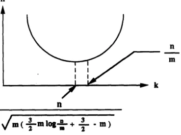
Let Cost2 = h(m,n,k). Since 0'~(m~n,k)Ok = ~ > 0, h(m,n,k) is a convex function in k. We

might choose the critical point k - ~ (see Fig. 4.1), which satisfies ~ --

~/,,(~m I.s ~ + g-m)

- - . ~ - - 2m s _T ₊1713 _{log ~ +}n 1712 _{= 0, to minimize the value of Cost2. However, the value is illegal}

because the premise says that k > ~ . Therefore, the minimal value of Cost2 is O(nm 2 log -~) 13

when we choose k -g.13 The time complexity is also O(rn s log g ) . Since the cost is higher than that for case 1, we have to abort this case. II

h n m k

/

il ~ m ( - ~ - - m l o g m-- ~ - + 3

_{"i- - m )}

Figure 4.1. The convex function h.

(9)

Algorithm for solving linear recurrences 195

5. C O N C L U S I O N

We have proposed a three-phase algorithm on the unshufl]e network to solve linear recurrences. Because the good computation property of C M - V s in sequential computation cannot be retained in parallel computation, when m is large the optimal cost

O(rnn)

of the problem is not met by our algorithm. The minimum cost achievable by the algorithm is

O(m2n)

with

O(m 2

log ~ ) execution time and O ( m - - ~ , ) processors. However, for the usual case when m is a small constant, the algorithm does achieve the optimal cost

O(n)

with O(logn) execution time and O(oI~gn) processors.

REFERENCES

I. D. A. Carlson and B. Sugla, Time and proce~or ei~cient parallel algorithn~ for recurrmlce equatiom and related problems, Prac. 1984 Int. Conf. on Parallel Proccssinl, IEEE Computer 5ocietl Press, Washingto,* D.C., 310--314 (1984).

2. D. A. Carkon and B. Sugla, Adapting shuffle-exchange llke parallel processing organizations to work as systolic arrays, Parallel Cornp~|ing 11 (1), 93-106 (1989).

3. K. L. Chung, F. C. Lin, and W. C. Chen, Parallel computation of continued fractions, under revision for J.

of Parallel and Distribwted Cornp~ting.

4. R. L. Graham, D. E. Knuth, and O. Patashnik, Concrete Mathematics, Addison-Wssley, Reading, MA, (1989).

5. P. M. Kogge and H. S. Stone, A parallel algorithm for the efficient solution of a general class of recurrence equations, IEEE Transactions on CornptLterJ C-22 (8), 786-793 (1973).

6. P. M. Kogge, Parallel solution of recurrence problems, IBM J. Research and Development, 138-148 (1974). 7. F. C. Lin and K. L. Chung, A cost-optimal parallel tridiagonal system solver, to appear in Parallel Corn.

p~ting.