Vectorized algorithms for solving special tridiagonal systems

P e r g a m o n

Computers Math. Applic. Vol. 32, No. 12, pp. 1-14, 1996 Copyright(~)1996 Elsevier Science Ltd Printed in Great Britain. All rights reserved 0898-1221/96 $15.00 + 0.00 PlI: S0898-1221 (96)00203.9

Vectorized Algorithms

for Solving Special Tridiagonal Systems

K u o - L I A N G C H U N G *

D e p a r t m e n t of I n f o r m a t i o n M a n a g e m e n t , N a t i o n a l T a i w a n I n s t i t u t e of T e c h n o l o g y No. 43, S e c t i o n 4, K e e l u n g R o a d , Taipei, T a i w a n 10672, R . O . C .

klchung©cs, nt it. edu. t w

W E N - M I N G YAN

D e p a r t m e n t of C o m p u t e r Science a n d I n f o r m a t i o n E n g i n e e r i n g N a t i o n a l T a i w a n U n i v e r s i t y

Taipei, T a i w a n 10764, R . O . C .

(Received November 1995; revised and accepted September 1996)

A b s t r a c t - - S o l v i n g special tridiagonal systems often arise in the fields of engineering and sci- ence. This special tridiagonal system is diagonally d o m i n a n t and circulant near-Toeplitz. This p a p e r presents two fast vectorized algorithms for solving special tridiagonal systems. B o t h algorithms employ the m a t r i x p e r t u r b a t i o n technique and have many computational advantages on vector su- percomputer. T h e related error analysis are also given. Some experimental results are illustrated on vector uniprocessor of t h e CRAY X-MP E A / l l 6 s e .

K e y w o r d s - - C i r c u l a n t near-Toeplitz systems, CRAY X-MP, Diagonally dominant, Error analyses, Tridiagonal matrices, Vectorized algorithms.

1. I N T R O D U C T I O N

In this paper, we are interested in the solution of the special tridiagonal system

A n x = b (1)

of order n on vector uniprocessor, where

a ~ "), An =

!3 ",/

and ]~1 > [a + 71. Solving (1) arises in many computational problems [1-7], in which it is one of the most time-consuming elements. T h e availability of vector supercomputers has had a significant impact on scientific computations [8-10]. The motivation of this research is to design efficient vectorized algorithms for solving (1).

* A u t h o r to w h o m all correspondence should be addressed.

T h e authors would like to t h a n k t h e help of the referees and Prof. E. Y. Rodin which led to an improved version of this paper. This research was supported in part by the National Science Council of R.O.C. under G r a n t s NSC85-2213-E011-009, NSC85-2121-M011-002, and NCHC86-08-015.

2 K.-L. CHUNO AND W.-M. VAN

In this paper, two fast vectorized algorithms for solving (1) are presented. Both new algorithms consist of three phases and only differ in the second phase. T h e first phase is a Toeplitz factor- ization of a slightly p e r t u r b e d m a t r i x of A n . T h e second phase is to solve the p e r t u r b e d problem in a highly vectorized way, b u t only scale x vector operations are involved, hence, it leads to a great deal of c o m p u t a t i o n a l saving. In the third phase, the solution to the original p r o b l e m is recovered from the solution to the p e r t u r b e d problem; this is called the u p d a t e procedure. Some error analyses are also given. In addition, some experimental results are illustrated on C R A Y X - M P E A / l 1 6 s e .

Section 2 presents our vectorized algorithms for solving (1) and the related error analyses. T h e i m p l e m e n t a t i o n s on the C R A Y X - M P EA/116se are illustrated in Section 3. Section 4 gives the conclusions.

2. V E C T O R I Z A T I O N S

2.1. T o e p l i t z F a c t o r i z a t i o n

T h r o u g h o u t the remainder of this paper, matrices are represented by uppercase letters, vectors by bold lowercase letters, and scalars by plain lowercase letters. T h e superscript 7- corresponds to t h e transpose operation; II * II denotes the sup-norm of one vector.

In order to avoid m e m o r y conflict in CRAY X - M P E A / l l 6 s e [11], we enlarge (1), t h e n p e r t u r b I /

it to A m x = b t, where m = pq (p denotes the length of one register file in the vector computer, i.e., the vector length), b r = (bl, b 2 , . . . , bn, 0 , . . . , 0) T, and

n n - - r / ~ A ' = = L ' U r, (2) a /3 -~ a /3 - d 1 a 7 L'-=- and U I = - d 1 a - d 1

which implies t h a t a - "~d = /J and - a d = a. This in t u r n implies t h a t d = - ( a / a ) and a = (/3+ x//32 - 4"ya)/2. Since we wish the matrices L ~ and U' to be diagonally dominant, we will select the sign so t h a t the absolute value of a is greater t h a n max(la[, 171). T h a t is, w h e n / 3 > ]a + V], we choose a = (/3+ V//32 - 4"ya)/2; when/3 <: - l a + 7 1 , we choose a -- ( / ~ - x//~ 2 - 4 7 a ) / 2 . Since one of our choices always makes ]a] > m a x ( l a l , IVI), hence, the bidiagonal Toeplitz matrices L ' and U ~ are diagonally dominant. T h e c o m p u t a t i o n of a and d provides the Toeplitz factorization of the m a t r i x A ~, which can be done in O(1) time.

2.2. S o l v i n g t h e P e r t u r b e d

System

2.2.1. T h e f i r s t m e t h o d

In this section, our first vectorized m e t h o d for solving A m x = t , b ~ in a highly vectorized way consists of two parts:

(1) vectorization of a lower bidiagonal Toeplitz system, L~ny t = bt; (2) vectorization of an upper bidiagonal Toeplitz system, U~m x~ = yr.

We would especially point out t h a t due to our m a t r i x p e r t u r b a t i o n technique, all the vector oper- ations involved are scaled by a constant, which is very i m p o r t a n t for the efficient i m p l e m e n t a t i o n on the vector computer.

V e c t o r i z e d A l g o r i t h m s 3

For convenience, we first describe t h e vectorized m e t h o d for solving the general lower bidiagonal Toeplitz s y s t e m ( L B T S ) , L m x = y, where

(:r )

Lm

= , for Irl >

8 r

8 r r n x m

and y = ( y l , y 2 , . . . , Y m ) T. In Section 2.1, we know t h a t m = pq. Therefore, we p a r t i t i o n t h e above L B T S into p L B T S ' s . E a c h L B T S can be w r i t t e n as

Lqxl(i) = y(O, for i = O, 1 , . . . , p - 1, (3)

, , , T y ( i )

where x '(i) = (X~q+l,X~q+2,...,Xiq+q) a n d = (Yiq+l,Yiq+2,...,Yiq+q) T. O u r vectorized s u b r o u t i n e for solving these p smaller L B T S ' s is shown in A p p e n d i x 1, where Loop-5 and Loop-20 can be vectorized with vector length p. Specifically, only scalar x vector o p e r a t i o n s are involved in this subroutine.

A f t e r solving x t in a vectorized way, we have

p - 1

L m x t -= y + s E X i q e i q + l , ( 4 )

i = 1 where ek = ( 0 , . . . , 0 , 1 , 0 , . . . , 0 ) T for 1 < k < m. Since

m - k n m e k = r e k + Sek+l, l < k < m , we have Let

)

s J ( _ r ) ek+j - ( s~J+ 1 \ i = o j=0 j=o = e k - - _ e k + t . e k + j + l

(5)

p - 1 t - 1 x = X' - r Z__ xiq z..~ - e i a . , + , , (6) i = 1 j = 0

where t d e n o t e s t h e length of t h e u p d a t e vector which will be discussed in Section 2.3, t h e solution v e c t o r x of (6) c a n be c o m p u t e d b y using t h e vectorized s u b r o u t i n e as shown in A p p e n d i x 2, where Loop-40 can be vectorized with vector length p - 1. O n l y scalar x vector o p e r a t i o n s are involved in this subroutine.

B y (5) a n d (6), we have L m x = y + s X ~ q e i q + l - 8 X i q e i q + l - - e i q + t + l i = l i = l p - 1 - _ e i q + t + l , i = l hence, 8 IILm x - y l l < - I s l r t llx']l" To e s t i m a t e IIx'll , we need t h e following lemma.

4 K.-L. C H U N G AND W.-M. V A N LEMMA 1. / f L =

:r

S r 8 ?-

ITI > Isl,

t h e n

I]L-'Yll -< 1 / ( I r l - IsI)I[YlI-

PROOF. See A p p e n d i x 3.

Using the above similar partition approach, it is easy to design our two vectorized subroutines, V U P P E R I ( r , s ) (vs. V L O W l ( r , s ) ) and U P D A T E U P P E R I ( r , s , t ) (vs. U P D A T E L O W I ( r , s , t ) ) , for solving the general u p p e r b i d i a g o n a / T o e p l i t z system (UBTS), Umx = y, where

u ~ =

r 8 r

7" S r

for I~1 > I~1-

For saving space, we omit the pseudo codes for these two subroutines.

R e t u r n to solve A m x ' ' = b'. Since A m = L i n G " , ' ' ' we first solve

LmY

' ' = b', w h e r e b ' = ( b l , b 2 , . . . , b n , 0 , - . . , 0 ) T, then solve U ' x ' ' = y ' . Using our previous vectorized m e t h o d s for

m - n

solving general lower and upper bidiagonal systems, the following algorithm is used to solve

' ' b'. A m i C * * * * * * t h e e n t r y a r r a y y r e p r e s e n t s v e c t o r b' C * * * * * * t h e e x i t a r r a y r e p r e s e n t s v e c t o r x' C A L L V L O W I ( I , - d ) C A L L U P D A T E L O W ( I , - d , t l ) C A L L V U P P E R l ( a , g a m m a ) C A L L U P D A T E U P P E R ( a , g ~ m m a , t 2 )

L E M M A 2. L e t Cl = 1/(1 - I d l ) and c2 = (1 + I d l ) b l ( 1 / ( l a l - h i ) ) ( ( 1 + Id])/(1 - Idl)), then

(

IlA~x'-

b'll <

elldl ''+1

+c2

Ilbll-

T h e t e r m cl[d[ tl+l will be less than ~, if tl is g r e a t e r than (log~ - l o g c l ) / l o g [d[ - 1; t h e t e r m c2[q/a[ t~+l will be less t h a n ~, if t2 is greater than ((log~ - logc2)/(log I f / a [ ) ) - 1. L e t c3 =

((1 + b / a l ) / ( l a l - h i ) ) ( ( 1 + Idl)/(1 - Idl)), t h e n i t

yields

IIx'll ~ a311bll.

PROOF. See A p p e n d i x 4.

L e m m a 2 will be used in the analysis of the u p d a t e phase in Section 2.3.

In the following section, based on the product expansion m e t h o d [12,13], we present the second vectorized m e t h o d for solving A m x -- b ' , where m = n, since we do not need the partition , , a p p r o a c h as described in Section 2.2.1.

Vectorized Algorithms 5 2.2.2. T h e s e c o n d m e t h o d

Now we describe our second vectorized method for solving L m x = y. All the vector operations involved are scaled only by a constant.

Since Lm =

r(I - E)

with

E =

/o

s 0

/

r

S 0

r s 0

the system L m x = y is equal to (I - E ) x -- ( 1 / r ) y . x can be obtained by computing x = (I + E2k) ..- (I + E 2 ) ( I +

E)((1/r)y)

because

Lmx = r(I -

E ) x

= r ( I - E ) ( I + E ) ( I + E 2 ) . . . ( I + E 2 k )

( l y )

Since we then have E 2k+l

(-;)

2k+1

( _ ~ ) 2~÷1

2k+1

yll <- ~

Ilyll.

(8)

IIZ~x

T h e relative residual

(llLmx-yll)/llYll

will be less than ~, if k is greater t h a n log(log ~/(log

Is/r[))

- 1 . Therefore, the computation of x (= x (k+l)) can be accomplished by the following iterative formula:

x.÷l~ _- (I + E2')x~'~ = x~" +

E2"x~'~, o < i < k,

(9)

with the initial assignment x (°) = ( 1 / r ) y .

From (8), we have [Ix(i+1)[[ _< (1 +

[s/r]2')llx(i)[].

Thus,

x(k+l) <_ ( 1 + s 2 k ) ( l q - l s 2 k - 1 ) . . . ( 1

1 -fs/rl 2~÷'

1

< ~ l l y l l .

+

- I l y l l

_r (10)

T h e formal vectorized subroutine for computing X ( k + l ) is shown in Appendix 5, where mainly scalar × vector operations are involved in this subroutine.

Similarly, it is easy to design our vectorized subroutine for solving the general UBTS system, U,~x = y. T h e corresponding vectorized subroutine is shown in Appendix 6, where mainly scalar × vector operations are involved in this subroutine.

6 K.-L. CHUNG AND W . - M . YAN

Using o u r previous two vectorized subroutines shown in A p p e n d i c e s 5 a n d 6 for solving gen- eral lower a n d u p p e r bidiagonal systems, respectively, t h e following p r o c e d u r e is used t o solve

' ' b ' .

A m x =

CALL VLOU2(I,-d,kl)

CALL VUPPER2 (a, gamma,k2)

L E M M A 3 . L e t c'1 = 1 a n d 5'2 : (1 + [d[)/(1 - [d[), t h e n w e have

[IA'x'- b'l[ _< @ldl 2~÷~ +c; Id'l ~ ' 1 ) Ilbll.

T h e t e r m

c'~ldl 2~'+~

will be less t h a n ~, i f kl is g r e a t e r t h a n l o g ( l o g ~ / l o g

Idl)

- 1; the t e r m c~]d'] 2~2+' wi]1 b e less t h a n ~, i f k2 is g r e a t e r t h a n l o g ( ( l o g ~ - l o g e ' 2 ) / l o g l d [ ) - 1. L e t c' 3 =

(1/([al- 17l)(1/(1 -Idl)),

then it follows that

IIx'll ~ c~llbll.

PROOF. See A p p e n d i x 7.

L e m m a 3 will be used in t h e following section. 2 . 3 . U p d a t e

A f t e r solving t h e p e r t u r b e d s y s t e m A m x -- ' ' b ' approximately, t h e a p p r o x i m a t e solution of x will be recovered from t h e p e r t u r b e d s y s t e m in this section.

L e t z ' _{= A m x - b ' , ~} , / _{= ( z l , z 2 , .} / , _{. . , z n) ,:~} I T _{= ( x ~ , x , 2 , . . . , n, ,} X / ~T and w _{= A n ~ - b . Since}

Wi ~" C~X~_ 1 -4- ~X~ -4- 7Xi.4_1! - bi = zi; for 1 < i < n,

Wl = ~ l X ~ -4- ~2X~ + Z3Xln -- 51, ( 1 1 )

l l l I I

wn ~3x1

= -4- ~2Xn_l

+

~ l X n -- bn,

w e h a v e H w - W l e l - Wnenll ~ IIzII ~_ IIz'[I. B y L e m m a 2, it follows t h a t

llAnO-b-Wlel- w,~e,,ll <_ IIz'Jl _< @lJdJ t~+~ +e2 ~t=)Ilbll-

02)

T h e value of [[z~[[ will be v e r y small w h e n tl a n d t2 are large enough. Therefore, t h e a p p r o x i m a t e solution of x to be d e t e r m i n e d equals ~ - p, where

A p - w l e l + W h e n . (13)

To solve p, we t r y to ignore t h e first a n d last equalities of the s y s t e m A p - w l e l -4- W h e n , t h e n we m u s t solve t h e recurrence relation: a p i - 1 -4- ~p~ -4- ~/P~+I -- 0 for 2 < i < n - 1. F r o m a - ~ d = ~. - a d = a , it follows t h a t c~ -4- Bd -4- 7d 2 = 0 and ~ -4- Bd' -4- o~d '2 = 0, where d' = - 7 / a . Naturally, if we t r y P l = (d, d 2 . . . d t3, 0 . . . 0) T, t h e n t3 n--t3 T A n P l = ( "~ld "4" ~2d2' t~d A- ~d2 "4" ~d3' " " " ' (~dtz-l "4" ~ d t ; ' ~ d t z ' O' " " " ' O'

n~-t3

] = l d ÷/32d2, O , . . . , O , ozd t3.1 ÷ / 3 d t S , a d t 3 , o . . . . , O , l ~ Y y ts n - t 3 = u e l . ÷ v e n + c ~ d t Z ( - d ~ e t 3 ÷ et3+l ) ,

Vectorized Algorithms 7 w h e r e u = (flld -t- fl2d 2) a n d v = ~ d . Similarly, if we t r y p2 = ( 0 , . . . , O, d t t * , . . . , d '2, dr) -c, t h e n n - - t 4 ~44

)

A n P 2 ---- u r e l 4- v t e n -1- ~ d tt4 - d ~ e n _ t 4 + l 4- e n _ t 4 , w h e r e v' = ( ~ [ d ' + f ~ d '2) a n d u ' = f~3d'. Let p = S p l + s ' p 2 , t h e n b y (14) a n d (15), we have (15) (16) A n p = ( s u + stu t) e l -t- ( s v + s ' v ' ) en + r, (17) w h e r e r = s a d t3 ( - d ( ~ / / a ) e t 3 + et3+l) -t- st'Td 't4 ( - d t ( o ~ / ' ) ' ) e n - t 4 + l -t- e n - t 4 ) .

C o m p a r i n g w i t h (13), we let s u + s t u r = Wl a n d s v + sty t = w n , a n d it follows t h a t

1211 vr - - W n U / S - - ?AC t - - V U r s' -- UWn - v w l (18) U V t - - y U / A n p = W l e l + W h e n ~- r. A f t e r d e t e r m i n i n g p , t h e s u b r o u t i n e for c o m p u t i n g x ( = :~ - p ) is shown in A p p e n d i x 8, w h e r e t h e a b o v e c o n c e r n i n g o p e r a t i o n s are t h e well-known p r e f i x - p r o d u c t o p e r a t i o n s .

F u r t h e r m o r e , c o m b i n i n g t h e vectorized s u b r o u t i n e s described in Section 2.2.1, a n d t h e a b o v e s u b r o u t i n e s h o w n in A p p e n d i x 8, o u r first vectorized a l g o r i t h m for solving (1) is c o n s t i t u t e d b y t h e following five subroutines.

CALL VLOWI (l,-d)

CALL UPDATELOW(I,-d, ti) CALL VUPPERI (a,g~mma)

CALL UPDATEUPPER (a, gmmm~a, t 2)

CALL FINAL(t3,t4)

Similarly, c o m b i n i n g t h e vectorized s u b r o u t i n e s described in Section 2.2.2, a n d t h e s u b r o u t i n e F I N A L ( t 3 , t4), o u r second vectorized a l g o r i t h m for solving (1) is shown below.

CALL gLOW2(l,-d,kl) CALL VUPPER2 (a, gamma, k2) CALL FINAL(t3,t4)

2.4. E r r o r A n a l y s e s

2 . 4 . 1 . F o r t h e f i r s t m e t h o d

T h e following t h e o r e m gives t h e error analysis of o u r first vectorized a l g o r i t h m for solving (1). THEOREM 4. L e t c4 = 1 + (11311 + If~21 + If~31)c3, c5 = 1 + (IBm] + 13~1 + 13~1)c3, c6 = (c41v'[ 4- c s l u ' l ) / ( l u v ' - v u ' l ) , a n d c7 = (cslul + c 4 1 v l ) / ( l u v ' - v u ' l ) , w e h a v e

[[Anx - bll

IIbtl

~__ (cl[d[ t ` + l 4- c2 Idt[ t2 4- csldl t3 4- (29 [ d t [ t 4 ) ,

w h e r e Cs = c6[a[ a n d c9 -- e7['7[. PROOF. See A p p e n d i x 9.

8 K.-L. CHUNe AND W.-M. YAN

For simplicity, b y T h e o r e m 4 we define t h e following n o t a t i o n s : tl(~) = m i n { t • N : clld[ t+l < ~/4}; t2(~) = rnin{t • N : c2[d'[ t < ~/4}; t3(~) = m i n { t • N : cs[d[ t < ~/4}; t4(~) = m i n { t • N : c91d'l t < ¢ / 4 } , where ~ is t h e u p p e r b o u n d of t h e relative residual. If max(t1 (~), t2(¢)) > n / p or m a x ( t 3 ( ¢ ) , t4(¢)) > n, t h e n our first vectorized a l g o r i t h m will break down w h e n t h e required relative t o l e r a n c e is sufficiently small a n d / o r t h e diagonal, d o m i n a n c e ratio is sufficiently close t o 2.

However, for some cases, our first vectorized a l g o r i t h m works well. For example, for conven- tional B-spline curve fitting [14,15], t h e c o r r e s p o n d i n g s y s t e m is of (1) with /31 -- 5, /32 = 1, /3 = 4, /33 = 0, a = 1, ~ = 1, /3~ = 5, /~ = 1, and/3~ -- 0. We have tl(~) = 11, t2(~) = 12, t3(~) = 13, a n d t4(~) = 13 for ~ = 10-6; we have tl(~) = 13, t2(~) = 14, t3(~) -- 15, a n d t4(~) = 15 for ~ = 10 -7. For closed B-spline curve fitting [14], t h e c o r r e s p o n d i n g s y s t e m is of (1) with/31 = 4, ~2 = 1 , 3 : 4 , J~3 = 1, a = 1, ~ ---- 1,/3~ = 4,/3~ = 1, a n d ~3~ = 1. We have tl(~) = 11, t2(~) --- 12,

t3(~) = 14, and t4(~) = 14 for ~ = 10-6; we have tl(~) = 13, t2(¢) = 14, t3(~) = 15, a n d t4(~) = 15 for ¢ -- 10 -7. F u r t h e r m o r e , let us examine t h e o t h e r two cases. If t h e s y s t e m is of (1) with/31 = 3, /32 = 1,/3 = 3,/33 = 1, c~ = 1, 7 -- 1,/3~ -- 3,/3~ = 1, and/3~ = 1, we have tl(~) = 16, t2(~) --- 17, t3(~) = 19, a n d t4(~) = 19 for ¢ = 10 -6, If t h e s y s t e m w i t h small diagonal d o m i n a n c e ratio is of (1) with/31 -- 2.1, /32 = 1, /3 = 2.1, /33 = 1, a = 1, 7 -- 1,/3~ = 2.1, /3~ = 1, and/3~ = 1, we have tl(~) = 52, t2(~) = 60, t3(~) = 68, a n d t4(¢) = 68 for ~ = 10 -6.

2.4.2. F o r t h e s e c o n d m e t h o d

In w h a t follows, we will discuss t h e error analysis o f our second vectorized a l g o r i t h m for solv- ing (1).

B y L e m m a 2 a n d (11), we have

Iw~l _~ ~llbll and

Iw,~l ~ c£11bll,

(19)

where c~ -- 1 4- (I/311 4- 1/321 + 1/331)c£ a n d ~5 = 1 4- (I/3~1 + I/3&l +

I/3&1)4,

B y (18) a n d (19), we have

Isl ~c~llbll

and

Is' I

<

c~llbll,

(20)

where c~ :

(c~lv'l +

c £ 1 u ' l ) / ( l u v ' - v u ' l ) a n d c~ =

(c£lul +

c ' 4 1 v l ) / ( l u v ' - v u ' l ) .

By

t h e variation of (ga) and (20), we have t h e following result.

THEOREM 5.

ilbl I + c; Id'[ 2k2+1 + csldl ts + c 9 Id'[ t4 , w h e r e c's = c'6[a[ a n d 4 = c~[71.

For simplicity, by (20) we define t h e following notations: Q(¢) --- m i n { t E N : [d[ 2¢+1 < ¢ / 4 } ; t2(~) = m i n { t E N :

c~ld'l 2¢÷1

< ¢ / 4 ) ;

t3(0

= m i n { t E N : c's[d] ¢ < ¢ / 4 } ; t4(¢) -- m i n { t E N :

c'gld'l ¢ < ¢/4}, where ¢ is t h e u p p e r b o u n d of the relative residual.

If m a x ( Q ( ~ ) , t 2 ( ~ ) ) > n or max(t3(~),t4(~)) > n, t h e n our second veetorized a l g o r i t h m will break d o w n w h e n t h e required relative tolerance is sufficiently small a n d / o r t h e diagonal domi- n a n c e ratio is sufficiently close t o 2.

However, for some cases, o u r second vectorized a l g o r i t h m works well. For t h e conventional B-spline curve fitting, we have t l ( ~ ) = 3, t 2 ( ~ ) ---- 3, t3(~) --- 13, a n d $4(~) -- 13 for ~ ---- 10-6; we have tl(~) = 3, t2(¢) = 3, t3(~) = 15, a n d t4(~) = 15 for ~ = 10 -7. For closed B-spline curve fitting, we have tl(~) = 3, t2(~) = 3, t3(¢) = 13, and t4(~) = 13 for ¢ = 10-6; we have t1(¢) -- 3, t2(¢) = 3, t3(¢) = 15, a n d t4(~) = 15 for f = 10 -7. F u r t h e r m o r e , let us e x a m i n e t h e previous two cases w i t h diagonal d o m i n a n c e ratios 3 / 2 a n d 2.1/2, respectively. For t h e first case, we have tl(~) = 3, t2(~) = 4, t3(~) = 19, a n d t4(¢) = 19 for ~ = 10 - 6 . For t h e second case, we have tl(~) -- 5, t2(~) -- 5, t3(~) -- 65, a n d t4(¢) = 65 for ~ = 10 -6.

V e c t o r i z e d A l g o r i t h m s 9

3. E X P E R I M E N T A L

R E S U L T S

T h e machine used in the numerical experiments is the CRAY X-MP EA/116se. T h e machine has a register-register architecture without the cache memory and has one vector processor which contains eight 64-bit vector registers of length 64. Memory is divided into 16 banks and each bank contains 1 M 64-bit words. Each bank requires 14 cycle time (one cycle time needs 8.5 nanosec- onds) before it is ready for another request. T h e peak performance is 235 M F L O P S (millions of floating-point operations per second). In order to avoid memory conflicts for some m, the value of m (> 512) can be selected as 64(2z + 1), where z is the smallest positive integer such that it satisfies t h a t 64(2z + 1) _> n. Here m = 64(2[n/128] + 1).

All of our testing data, b's are generated by a random number generator, a function call r a n f 0 , and each entry of b is ranged from 0 to 1. Our two vectorized algorithms are coded by CRAY Fortran 77 language. T h e operating system used here is UNICOS 6.1.6 and the compiler is called CF77.

Let A i l = Ai(2.5), Ai2 = A{(2.7), and Ai3 = Ai(3) for i = 1, 2, where

A1(/3) =

I

1 ~ 1

1

a n d In addition, we let a n d A2(/3) = 1 A 1 4 - - 4 1 1 4 1 5 1

:/

1 4 1 A 2 4 --- 1 4 1 1

which are derived from the conventional B-spline curve fitting problem and have been discussed in Section 2.4. When running our two algorithms on CRAY X-MP E A / l l 6 s e , the performance is illustrated in Table 1 and Table 2, respectively•

T a b l e 1. F i r s t a l g o r i t h m ' s p e r f o r m a n c e o n C R A Y X - M P E A / l l 6 s e . n p q t i m e ?'11 7"12 7"13 r14 7'21 ?'22 r23 /'24 2 0 4 8 64 33 0 . 1 8 10 - 8 10 - 1 ° 10 - 1 1 10 - 1 1 10 - s 10 - 1 0 10 - 1 1 10 - 1 1 4 0 9 6 6 4 65 0 . 2 7 10 - s 10 - l ° 10 - 1 1 10 - 1 1 10 - s 10 - 1 ° 10 - 1 1 10 - 1 1 8 1 9 2 6 4 129 0 . 4 5 10 - 8 10 - l ° 10 - 1 1 10 - 1 1 10 - s 10 - 1 ° 10 - 1 1 10 - 1 1 1 6 3 8 4 6 4 2 5 7 0 . 8 1 i 0 - s 10 - 1 ° i 0 - I I 10 - 1 1 10 - 8 10 - 1 ° 10 - 1 1 10 - 1 1

10 K.-L. CHUNG AND W.-M. VAN

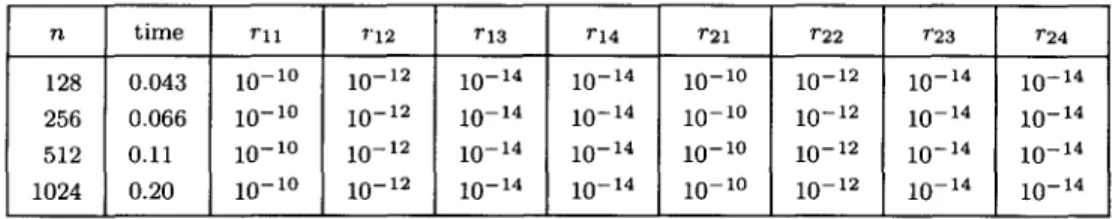
Table 2. Second algorithm's performance on CRAY X-MP EA/ll6se.

n time 128 0.043 256 0.066 512 0.11 1024 0.20 r l l 10-1o 10-10 10-1o 10-1o 7'12 r13 r14 r21 r22 r23 r24 10-12 10-14 10-14 10-10 10-12 10-14 10-14 10-12 10-14 10-14 10-10 10-12 10-14 10-14 10-12 10-14 10-14 10-10 10-12 10-14 10-14 10 -12 10-14 10-14 10-10 10-12 10-14 10-14

In Tables 1 and 2, the symbols n, p, and q x q denote the size of b, the n u m b e r of the blocks, the size of one block. T h e symbol ' t i m e ' in t e r m s of millisecond, represents the t i m e spent in the first vectorized algorithm. T h e symbol rij for 1 < i < 2 and 1 < j < 4 represents the s u p - n o r m of the relative residual corresponding to Aij. In Table 1, by T h e o r e m 4, we select tl -- t2 -- t3 = t4 = 30; in Table 2, by T h e o r e m 5, we select kl = k2 -- 5 and t 3 = t4 -- 30.

4. C O N C L U S I O N S

This p a p e r has presented two fast vectorized algorithms for solving special tridiagonal s y s t e m s and has analyzed the error analyses. Due to our m a t r i x p e r t u r b a t i o n technique, all the vector operations involved in the two algorithms are scaled by a constant, which is very i m p o r t a n t for the efficient i m p l e m e n t a t i o n on the C R A Y X-MP. Some experimental results d e m o n s t r a t e the p e r f o r m a n c e of our two vectorized algorithms. Our results can be applied to solve the quadratic B-spline curve fitting problem [16,17], the parabolic P D E [4] problem, and so on, since these problems belong to the t y p e of special tridiagonal Toeplitz systems.

Using the same m a t r i x p e r t u r b a t i o n m e t h o d proposed in this paper, the parallel algorithms for solving (1) on hypercubes [18] and the B-spline surface fitting [19], respectively, have been developed. In addition, the results of this p a p e r can also be applied to solve the diagonally d o m i n a n t block tridiagonal s y s t e m to achieve b e t t e r performance. It is interesting to employ the other parallel tridiagonal solvers [20,21].

A P P E N D I X

1

SUBROUTINE VLOWI(r, s) real r, s

C*****the entry array y represents vector y C*****the exit array y represents vector x'

do 5 i=0, p-i

y (i*q+l) = (i/r) *y (i*q+l)

5 continue do l0 j = 2 , q do 20 i = 0 , p - i y ( i * q + j ) = ( i / r ) * ( y ( i * q + j ) - s * y ( i * q + j - 1 ) ) 20 c o n t i n u e 10 c o n t i n u e

A P P E N D I X

2 SUBROUTINE UPDATELOWI(r,s,t) real r,s integer t

C******the entry array y represents vector x' C******the exit array y represents vector x

temp=l

do 30 j=0,t-I temp=temp*(-s/r)

Vectorized Algorithms 11

40 30

do 40 i=l,p-I

y (i*q+j+l) =y(i*q+j+l) +y(iq) *temp

c ont inue continue A P P E N D I X 3 Let L - l y = x, t h e n L x = y, i.e., r x l = y l , ( 3 a ) S X i - 1 ~- TXi : Yi, i > 1. (3b)

I f ]]Xli = [Xl[, t h e n by (3a), we have [lY[[ -> [Y,I = I r x l ] = [r[ [[xl[. If [Ix[I --- Ixil for some i > 1,

t h e n by

(3b)

and the triangular inequality, we have

IlYll -> lYil k I r x i l -

18Xi-ll

> I"1 Ilxll- Isl Ilxll

= ( I r l - Isl)llxll.

We complete the proof and have Ilxll _< (1/(Ir I - Isl))llyll. A P P E N D I X 4

Taking the triangular inequality on b o t h sides of (6), since I s / r l < 1, it yields Ilxll_< ( 1 + s ) l l x , ll.

Applying L e m m a 1 to (3), we have

IIx'(*)l I ~

1/(It I -Isl)lLy(*)ll, Thus, we obtain

Ilx'l] = m a x x '(i) l_<~<p 1 y(O < m a x - - l_<~<_plrl isl 1

< - - I l y l l .

- M - Isl Furthermore, by (7) we have (4a) by (4a), we have 1 + Is/rl Hxll-< T ~ - - ~ IlyH- (4c)

By (4b), (4c), and their variations, the bound of the sup-norm of the residual vector Amx~ t _ b ~ is derived by

HXmX' - b'll _< IlL" (U'~x' - Y')ll ÷ l I L l Y ' - b'll <_ (1 + I d l ) H U t m x ' - Y'II + l I L l Y ' - b'll

<_ (1 + Idl)17 [ 2 t2 1 1

a lal - I"/---'~l [lY']I + Idl t ' + l 1 - [d--~l <__ ( ( 1 + Idl)171 2 t2 1 1 + Id I a lal -1"71 1 - I d l + l d l t l + l

IIb'll

1)

1 - I d l Ilbl[" s t 1

12 K.-L. CHUNG AND W.-M. YAN

L e t c1 ~--- 1 / ( 1 - - Idl) and c2 -- (1 +

Idl)]vl(1/(Jal-

h i ) ) ( ( 1 +

Idl)/(1

- I d l ) ) , t h e a b o v e b o u n d is

simplified by

[ , A ' x ' - b ' [ , < (clldl t1+1 + c 2

a

7-t2) ]]b]l.

(4d)

T h e t e r m cl[dl t~+l will be less t h a n ~, if ~;1 is greater t h a n (log~ - l o g c l ) / l o g [d[ - 1; t h e t e r m c217/a[ t2+1 will be less t h a n ~, if t2 is g r e a t e r t h a n (log~ - l o g c 2 ) / ( l o g Iv/a[) - 1.

B y (4c) a n d its variation, we have

Ilx'll

<

_{- T ~ [ - ~ - ~}

1

+

b/al

_[ly'll

< 1 + l'7/a[ 1 + Id[ ]lb, ll "

Let c3 = ((1 +

b/al)/(lal-

I~J))((1 + Idl)/(1 - ] d [ ) ) , t h e n it yields

IIx'll _< 31FblI.

A P P E N D I X

5

S U B R O U T I N E VLOW2 (r, s, k) integer k real r,s p=l t e m p = - s / r C * * * * * V e c t o r operation x [1 :n] = ( 1 / r ) * x [1 :n] do I0 i=0,k C * * * * * C o m p u t e (15) in a vectorized way x [l+p : n] =x [l+p : n] +t emp*x [I : n-p] t e m p = t e m p * t e m p p=p*2 10 c ont inue 10

A P P E N D I X

6

S U B R O U T I N E VUPPER2 (r, s, k) integer k real r, s p=l t e m p = - s / r x [i :n] =(I/r)*x [i :n] do i0 i=0,k x [ 1 :n-p] =x [ I :n-p] +t emp*x [ l+p: n] t emp=t emp * t emp

p=p*2 c ont inue

A P P E N D I X

7

B y (8), (10), a n d their variations, t h e b o u n d of t h e s u p - n o r m of t h e residual v e c t o r Amxl , _ b t isderived b y

Vectorized Algorithms 13

J l A ' ~ x ' -

b'll _<

<_

<_

<_

J]L~m (U'mx' - Y')]I + IIL~my ' - b'lJ

(1 + [dl)IIU'~x' - Y'II + l I L l y ' - b'll (I + Idl)Id'l 2~+' IIY'IJ + JdJ 2~2+~ llb'll

(1 + Idl)Id'J 2~+1 ~

Ilb'll + Idl 2~+~ IIb'll

1 - I d l

(

(1 + Idl)Id'l 2~1+1 1

-Id----~

1

+ Id12~+l

) IIb]l.

Let c~ = I and c~ = (1 +

Idl)/(1 -IdJ),

t h e n the b o u n d is simplified by

J l A ' x ' - b'll <_ (cildl2~'+' + c~ Id'l 2~+') ilbll.

(7a)

T h e t e r m c~JdJ 2~1+1 will be less t h a n 4, if kl is greater t h a n

log(logS/logJdl)

- 1; t h e t e r m

c'2]d'] 2~2+~

will be less t h a n 4, if k2 is greater t h a n log((log ~ - l o g c ~ ) / l o g ]d]) - 1. F r o m (10) a n d its variation, we have

1

Jlx'JJ

< JaJ- i"/~---~

jjy'jj

1 1

< - - - - i l b i l .

- l a J -

l'yl

1

-Idl

Let c~ =

(1/(lal

- J ' y l ) ) ( 1 / ( 1 - I d l ) ) , t h e n t h e simplified b o u n d is given b y

IIx'll ~ 411bll.

(Tb)

A P P E N D I X 8 SUBROUTINE F I N A L ( t 3 , t 4 ) i n t e g e r t 3 , t 4 temp=d do 10 i = l , t 3

x [i] =X [i] - t emp*s t e m p = t e m p * d

i0 c o n t i n u e

C * * * * * d p r e p r e s e n t s d' in t h e c o n t e x t

temp=dp

do 20 i=n,n+l-t4

C*****sp represents s' in the context x [i] =X [i] -temp*sp

temp=temp*dp

20 continue

A P P E N D I X 9 B y x -- ~ - p, (16), (17), a n d (18), we have

A n x - b -- A n ~ - b - Amp

= Anx

- b - Wlel -

When

sc~dtS(_d_~ets+ets+l)_S,,Td,t, ( ,c~

en-t4)

- - d - - e n _ t 3 + 1 + -y I m m e d i a t e l y , it yields 1oL N A n x - b N < , , z ' H +

sadtZ(-d~ets+ets+l)+S"ydn4(-d~en-t4+l+en-t4)

(9a)

14 K.-L. CHUNG AND W.-M. VAN

B y (11) and L e m m a 2, we have

IWll ~ c411bll and Iwnl

~

callbll, (9b)

where c4 = 1 + (1~1[ + 1~2[ + 1~31)c3 and c5 = 1 + (IBi] + IZ~I + I~hl)c3. B y (18) and (gb), we have

[sl ~< c6llbll

and

Is'l - cTIFbll,

(9c)

where c6 =

(e41v'l

+

cslu'l)l(luv'

- v u ' l ) and c7 = (cslul

+

c41vl)l(luv'

- v u ' l ) . B y (ga) and (9c),

it follows t h a t

IIAnx - bll _{< / [Clldl t1+1 + c2 Id'l t2 + cs[dl t3 + c9}

Id'lt'),

_{~ (9d)}

Ilbll where cs =

c61~1

and c9 =

c71~1.

R E F E R E N C E S

1. J.J. Dongarra, C.B. Moler, J.R. Bunch and G.W. Stewart, L I N P A C K User's Guide, SIAM Press, Pennsyl- vania, (1979).

2. D. Fischer, G. Golub, O. Hald, C. Levia and O. Widlund, On Fourier-Toeplitz methods for separable elliptic problems, Mathematics of Computation 28 (126), 349-368 (1974).

3. O.B. Widlund, On the use of fast methods for separable finite difference equations for the solution of general elliptic problems, In Sparse Matrices and Their Applications, (Edited by D.J. Rose and R.A. Willoughby), pp. 121-131, P l e n u m Press, New York, (1972).

4. G.D. Smith, Numerical Solution of Partial Differential Equations: Finite Difference Methods, Oxford University Press, (1985).

5. R. R o b e r t s and C.T. Mullis, Digital Signal Processing, Addison-Wesley, Reading, MA, (1987). 6. R.W. Hockney and C.R. Jesshope, Parallel Computers 2, A d a m Hilger, Bristol, (1988).

7. R.F. Boisvert, Algorithms for special tridiagonal systems, S I A M J. Sci. Stat. Comput., 12, 423-442 (1991). 8. J. Ortega, Introduction to Parallel and Vector Solution of Linear Systems, Plenum Press, New York, (1988). 9. J.J. Dongarra, I.S. Duff, D.C. Sorensen and H.A. van der Vorst, Solving Linear Systems on Vector and

Shared Memory Computers, SIAM Press, Pennsylvania, (1991).

10. G. Golub and J. Ortega, Scientific Computing: An Introduction to Parallel Computing, Academic Press, New York, (1993).

11. Supercomputer Programming (I): Advanced Fortran: Architecture, Vectorization, and Parallel Computing, Working m a n u a l for CRAY X - M P EA/116se, (1991).

12. O. Axelsson and V. Eijkhout, A note on the vectorization of scalar recursions, Parallel Comput. 3, 73-83 (1986).

13. H.S. Stone, An efficient parallel algorithm for the solution of a tridiagonal linear system of equations, J. ACM. 20, 27-38 (1973).

14. R.H. Bartels, J.C. B e a t t y and B.A. Barsky, An Introduction to Splines for Use in Computer Graphics and Geometric Modeling, Morgan Kaufmann, California, (1987).

15. K.L. C h u n g and L.J. Shen, Vectorized algorithm for B-spline curve fitting on CRAY X-MP EA/16se, Presented at the I E E E Conf. on Supercomputing, November 1992, pp. 166-169.

16. B. P h a m , Quadratic B-splines for automatic curve and surface fitting, Comput. ~J Graphics 13, 471-475 (1989).

17. K.L. C h u n g and W.M. Yah, Computing quadratic B-spline curve fitting on CRAY X-MP, In Proc. National Computer Symposium, Chiayi, R.O.C., December 1993, pp. 401-407.

18. K.L. Chung, W.M. Yan and J.G. Wu, A parallel algorithm for solving special tridiagonal systems on ring networks, Computing 56 (4), 385-395 (1996).

19. K.L. Chung and W.M. Yan, Parallel B-spline surface fitting on mesh-connected computers, J. Parallel and Distributed Computing 35, 205-210 (1996).

20. R.W. Hockney, A fast direct solution of Poisson's equation using Fourier analysis, J. ACM. 12, 95-113 (1965).