A repetitive learning method based on sliding mode for robot control

T. S. Liu

W. S. Lee

Department of Mechanical Engineering, National Chiao Tung University, Hsinchu 30010, Taiwan e-mail: tsliu@cc.nctu.edu.tw

A Repetitive Learning Method

Based on Sliding Mode

for Robot Control

In order to make a robot precisely track desired periodic trajectories, this work proposes a sliding mode based repetitive learning control method, which incorporates character-istics of sliding mode control into repetitive learning control. The learning algorithm not only utilizes shape functions to approximate influence functions in integral transforms, but also estimates inverse dynamics functions based on integral transforms. It learns at each sampling instant the desired input joint torques without prior knowledge of the robot dynamics. To carry out sliding mode control, a reaching law method is employed, which is robust against model uncertainties and external disturbances. Experiments are per-formed to validate the proposed method.关S0022-0434共00兲02001-3兴

1 Introduction

A learning system is capable of improving its performance over time by interaction with its environment. A learning control sys-tem is designed so that its learning controller can improve the performance of closed-loop systems by generating command in-puts to plants and utilizing feedback information from plants. Rather than proportional-derivative 共PD兲 type learning control methods in the past 关1兴, fuzzy learning control 关2兴 and neural network based learning controller关3兴 have been presented. Yang and Asada关4兴 proposed an excitation scheduling method to enable an impedance control law to learn quasi-static, slow modes in the beginning, followed by learning faster modes. Similar to control-lers presented by Horowitz关5兴 and Messner et al. 关6兴, a repetitive robot controller was implemented with Cartesian trajectory de-scription关7兴. A structured singular value method was also applied to determine stability and performance robustness of repetitive control systems关8兴.

This study presents a sliding mode based repetitive learning control approach to robot control. The advantages of using sliding mode control instead of PD control for feedback portion of a repetitive learning control include:共1兲 the robust property of slid-ing mode control dealslid-ing with model uncertainties;共2兲 the flex-ibility in using sliding mode control. It is known that, in general, the transient dynamics of a variable structure control system关9兴 is accounted for by a reaching mode followed by a sliding mode 关10兴. Therefore the design involves, first, the design of an appro-priate sliding surface and a reaching mode method for the desired sliding mode dynamics, and second, the design of a learning al-gorithm to ensure asymptotically stability.

Sliding mode based repetitive learning control focuses on learn-ing rules that estimate feedforward terms共inverse dynamic func-tions兲. A class of function identification for learning algorithm compensation based on integral transforms was presented by Messner et al.关6兴. This study employs a set of shape functions to approximate influence functions and estimates inverse dynamics functions based on integral transforms. The inverse dynamics function is estimated by the integral of a predefined kernel multi-plied by an estimated influence function. The influence function used in integral transforms is approximated by a set of linear shape functions and this influence function is in turn represented by corresponding coefficients. An adaptation law employing

ker-nel functions, sliding surfaces, and shape functions is thus devel-oped in this study to update the coefficients associated with influ-ence functions.

2 Tracking Control of Manipulator

In general, the equation of motion for a n-axis manipulator can be expressed as

M共q兲q¨⫹C共q,q˙兲q˙⫹G共q兲⫹d共q,q˙兲⫽u (1)

where q, q˙, and q¨ are, respectively, the n⫻1 joint position, ve-locity, and acceleration vectors, u represents the n⫻1 torque vec-tor generated by actuavec-tors, M (q) is the symmetric positive defi-nite generalized inertia matrix, C(q,q˙) is the force共torque兲 vector resulting from Coriolis and centripetal accelerations, G(q) is the generalized gravitational force vector, and d(q,q˙) denotes the dis-turbance. Define a 2n-dimensional state vector x as

x⫽

冋

x1 x2

册

⫽

冋

q q˙

册

Thus Eq.共1兲 can be written as

x˙⫽A共x兲⫹B共x兲u⫹␯共x兲 where A共x兲⫽

冋

_⫺M⫺1_{共x兲C共x兲x}x2 2⫺M⫺1共x兲G共x兲

册

B共x兲⫽

冋

0 M⫺1共x兲

册

and the disturbance is expressed by

␯共x兲⫽

冋

_⫺M⫺10_{共x兲d共x兲}

册

2.1 Sliding Mode Control. The manipulator is demanded to track a desired motion qd(t). Define an error vector

e⫽

冋

e˙ e

冕

0 t edt

册

where e⫽q⫺qdand e˙⫽q⫺q˙d. A sliding surface s of n

dimen-sions is of the form: Contributed by the Dynamic Systems and Control Division for publication in the

JOURNAL OFDYNAMICSYSTEMS, MEASUREMENT,ANDCONTROL. Manuscript received by the Dynamic Systems and Control Division April 15, 1999. Associate Technical Editor: E. A. Misawa.

s共e兲⫽C共e兲⫽关I ⌳ ⌫兴

冋

e˙ e

冕

0 t edt

册

⫽e˙⫹⌳e⫹⌫

冕

0 t edt (2)

where both⌳ and ⌫ are positive definite matrices. In addition, a reaching law关11兴 is defined as

s˙⫽⫺Q sgn共s兲⫺Ks (3)

where gains Q and K are diagonal matrices with positive elements qiand ki, respectively. Chattering can be reduced by tuning qi

and ki in this reaching law. Near the sliding surface, si⬇0. It

follows from Eq. 共3兲 that 兩s˙i兩⬇qi. By using a small gain, the

chattering amplitude can be reduced. However, qicannot be

cho-sen equal to zero since the reaching time would become infinite. Moreover, when the state is not near the sliding surface a large ki

is employed to increase the reaching rate. Taking the time derivative of Eq.共2兲 gives

s˙⫽e¨⫹⌳e˙⫹⌫e

⫽⌳e˙⫹⌫e⫺q¨d⫺M共q兲⫺1共C共q,q˙兲q˙⫹G共q兲⫹d共q,q˙兲⫺u兲

(4) Equating Eqs.共3兲 and 共4兲 yields control input

u⫽M共q兲兵⫺Q sgn共s兲⫺Ks⫺⌳e˙⫺⌫e⫹q¨d其

⫹C共q,q˙兲q˙⫹G共q兲⫹d共q,q˙兲 (5)

2.2 Sliding Mode Based Repetitive Learning Control. Tracking control is aimed at following a prescribed trajectory as closely as possible. Using inverse kinematics one can obtain joint position, velocity, and acceleration vectors denoted by qd, q˙d,

and q¨d, respectively. The desired torque input of a manipulator,

denoted by wd(.):R⫹→Rn, is defined as

wd共t兲⫽M共qd兲q¨d⫹C共qd,q˙d兲q˙d⫹G共qd兲⫹d共qd,q˙d兲 Definition: Let Ck(T) denote a subset of C(T) 共which is the

space of continuous T-period functions wd:R⫹→Rn兲 such that

every wdis piecewise continuously differentiable, and

sup

t苸关0,T兴

冏

d

dtwd共•兲

冏

⭐k

Given a collection for shape functions兵⌽i其and␧⬎0, there exists

a finite number of shape functions兵⌽0,⌽1,⌽2,...,⌽N其that

uni-formly approximate members of Ck(T) within␧⬎0, i.e., for

ev-ery wd苸Ck(T), there exists constant vectors C0,C1,C2,...,Cn 苸Rn_{such that} sup t苸关0,T兴

冏

wd共t兲⫺

兺

i⫽0 N Ci⌽i

冏

⬍␧

To estimate the desired torque wd(t), it can be approximated by a

linear combination of appropriately selected period shape func-tions⌽i. Hence,

wd共t兲⬵

兺

i⫽0 N

Ci⌽i共t兲 (6)

where Ci苸Rn represent unknown coefficient vectors for each

shape function⌽iat an instant, and N denotes the total number of

shape functions. The estimated feedforward term is generated by determining the coefficient vectors Cˆi关7兴, i.e.,

wˆd共t兲⫽

兺

i⫽0 N

Cˆi⌽i共t兲 (7)

The coefficient vectors are updated on-line by conducting the fol-lowing estimation law关7兴:

d

dtCˆi共t兲⫽⫺KL⌽i共t兲s i⫽1,2, . . . ,N (8) where KL is a constant positive definite matrix.

Another approximation of the ideal feedforward compensation term can be represented by

wd共t兲⫽

冕

0

T

K共t,␶兲I共␶兲d␶ (9)

where the function K(•,•):R⫻关0,T兴 is a known Hilbert-Schmit kernel that satisfies

冕

0

T

K共t,␶兲2d␶⫽k⬍⬁ K共t,␶兲⫽K共t⫹T,␶兲 (10)

whereas the influence function I(•):关0,T兴→Rn _{is unknown. If a}

kernel function is chosen to satisfy Eq.共10兲, then the feedforward term wd(t) can be estimated by influence function I(•). The

fol-lowing function adaptation law for estimating the unknown func-tions wd(t) and I(•) was presented by Messner et al.关6兴:

wˆd共t兲⫽

冕

0 T K共t,␶兲Iˆ共t,␶兲d␶ (11) ⳵ ⳵tIˆ共t,␶兲⫽⫺KLK共t,␶兲s (12)

The estimated wˆd(t) is hence indirectly updated by the adaptation

of Iˆ(t,␶), which is the estimate of the influence function I(␶). In the integral transform estimation, the feedforward term wˆd(t) is estimated through updating the influence function Iˆ(t,␶)

according to the learning law Eq.共12兲. However, if the influence function, which belongs to the space of continuous T-period func-tions, satisfies sup t苸关0,T兴

冏

Iˆ共t,␶兲⫺

兺

i⫽0 N Cˆi共t,␶兲⌽i共␶兲

冏

⬍␧,

it can be expressed by a set of shape functions. The unknown influence function is proposed as

Iˆ共t,␶兲⫽

兺

i⫽0 N

Cˆi共t,␶兲⌽i共␶兲 (13)

and the coefficient adaptation law becomes ⳵

⳵tCˆi共t,␶兲⫽⫺KLK共t,␶兲⌽i共␶兲s (14)

where ⌽i(•) denotes a shape function and Cˆi(•) its associated

coefficient. The advantage of the above learning rule is that only the associated coefficients for shape functions are updated in es-timating the influence function, which can be in turn obtained by a linear combination of shape functions. It is unnecessary to save all influence function values at every sampling instant, thus com-puter memory space can be saved. Since the value of influence function Iˆ(t,␶) is updated on the basis of previous value Iˆ(t,␶ ⫺⌬␶), the property of ‘‘interpolating’’ is achieved.

2.3 Stability Analysis. The stability of the present control method for the robotic model represented by Eq.共1兲 depends on the following conditions.

Condition 1: There exists an influence function ␣(t,␶), such that M共q兲␷˙⫹C共q,q˙兲␷⫹G共q兲⫹d共q,q˙兲⫽

冕

0 T K共t,␶兲␣共t,␶兲d␶ (15) where␷(t)苸Rn_{is a vector of smooth functions.}

Condition 2: Using a proper definition of matrix C(q,q˙), both M (q) and C(q,q˙) in Eq.共1兲 satisfy

xT共M˙⫺2C兲x⫽0 ᭙x苸Rn

Hence, ( M˙⫺2C) is a skew-symmetric matrix. In particular, the element of C(q,q˙) can be defined as

Ci j⫽ 1 2

冋

q˙ T⳵Mi j ⳵q ⫹k

兺

⫽1 n

冉

⳵Mik ⳵qj⫺ ⳵Mjk ⳵qi

冊

q˙k

册

(16)

Condition 3: In robot control systems, the disturbance d(q,q˙) due to friction, sensor noise, etc. is assumed to be bounded. Gen-erally speaking, unmodeled dynamics is bounded as follows:

储d储⭐L0⫹L1储e˙储⫹L2储e储 where L0, L1, and L2are positive constants.

Remark: If the structure conditions presented above are satis-fied, a sliding mode based repetitive learning controller for achieving the trajectory tracking can be realized.

In the current study, the norm of vector x is defined as 储x储⫽

冉

兺

i⫽1 n xi 2

冊

1/2

and the norm of matrix A is defined as 储A储⫽共 max

eigenvalue

AT_A兲1/2

The singular value of matrix A is defined as ␣(A) ⫽(eigenvalue(AT

A))1/2and␣min(A) denotes the smallest singular value. For positive definite matrix A⫽AT, the matrix property 关12兴

xTAx⭓␣min共A兲储x储2 (17)

will be employed in this work to formulate the learning control method.

In the following, a brief overview of the proposed sliding mode based repetitive learning controller is given. The design problem for the proposed sliding mode based repetitive learning controller is described as follows: For any given desired trajectory qd 苸Rn_{, q˙}

d苸Rn, and q¨d苸Rn, with some or all of the manipulator

coefficient vectors unknown, derive a controller for the actuator torque共force兲, and an adaptation law for the unknown coefficient vectors, such that the manipulator joint position q(t) precisely tracks qd(t).

To ensure the convergence of the trajectory tracking, define a reference velocity vector q˙ras

q˙r⫽q˙d⫺⌳e⫺⌫

冕

0

t

edt (18)

where both⌳ and ⌫ denote positive definite matrices whose ei-genvalues are strictly in the right-half plane. Therefore, the sliding surface s defined in Eq.共2兲 can be expressed by

s⫽e˙⫹⌳e⫹⌫

冕

0

t

edt⫽q˙⫺q˙r (19)

Consider the plant defined in Eq.共1兲, a repetitive learning control-ler using sliding mode feedback control is proposed, i.e.,

u⫽wˆd共t兲⫺Q sgn共s兲⫺Ks (20)

where wˆd(t) can be estimated by the linear combination of shape

functions Eq.共7兲 or by the integral of kernel function and influ-ence function Eq.共11兲. The adaptation laws can be found in Eqs. 共8兲 and 共12兲. Treating s⫽0, where s is defined in Eq. 共19兲, as a sliding surface, by combining Eqs. 共1兲 and 共18兲 and using the property that s⫽q˙⫺q˙r, which follows from Eqs.共2兲 and 共18兲, the

sliding mode equation reads

M s˙⫽

冕

0 T K共t,␶兲Iˆ共t,␶兲d␶⫺

冕

0 T K共t,␶兲␣共t,␶兲d␶ ⫺Cs⫺Ks⫺Q sgn共s兲⫺d (21)

where the following definition is used, which satisfies Condition 1,

M共q兲q¨r⫹C共q,q˙兲q˙r⫹G共q兲⫽

冕

0

T

K共t,␶兲␣共t,␶兲d␶ A generalized Lyapunov function is chosen as

V共t兲⫽12s

T M s⫹12e

T

KLe (22)

where KL⫽␴SI with ␴S⬎0. Taking the time derivative of Eq. 共22兲 gives

V˙⫽sT_{M s˙⫹s}T_Cs⫹eT_K

Le (23)

Substituting Eq. 共20兲 into Eq. 共23兲 and employing Condition 2 give V˙⫽sT

再

冕

0 T K共t,␶兲关Iˆ共t,␶兲⫺␣共t,␶兲兴d␶⫺Ks⫺Q sgn共s兲⫺d

冎

⫹eT_K Le˙ (24)

Now choosing⌳ and ⌫ such that sT␣(t,␶)⬎sTIˆ(t,␶) yields V˙⭐⫺sTKs⫺sTQ sgn共s兲⫺sTd⫹eTKL

冉

s⫺⌳e⫺⌫

冕

0

t edt

冊

(25) From Condition 3, one has

⫺sT_d⭐储s储

冋

_L 0⫹L1

冉

储s储⫹⌳储e储⫹⌫

冐

冕

0 t edt

冐

冊

⫹L2储e储

册

⭐L0储s储⫹L1储s储2⫹关␭M共⌳兲L1⫹L2兴储s储储e储 ⫹L1␭M共⌫兲储s储

冐

冕

0 t edt

冐

(26)

where␭M(⌳) denotes the maximum eigenvalues of ⌳. It follows

that V˙ ⭐⫺关␭m共K兲⫺L1兴储s储2⫹关␴S⫹␭M共⌳兲L1⫹L2兴储s储储e储 ⫹L1␭M共⌫兲储s储

冐

冕

0 t edt

冐

⫺␴S␭m共⌫兲储e储

冐

冕

0 t edt

冐

⫺␴S␭m共⌳兲储e储2⫹关L0⫺␭m共Q兲兴储s储 (27)

where ␭m(•) denotes the minimum eigenvalue of a matrix. A

further manipulation of Eq.共27兲 leads to

V˙⭐⫺

冋

储s储 储e储

冐

冕

0 t edt

冐

册

R

冋

储s储 储e储

冐

冕

0 t edt

冐

册

⫺␭m共K兲 2

冋

储s储⫺ L0⫺␭m共Q兲 ␭m共K兲

册

2 ⫹关L0⫺␭m共Q兲兴2 2␭m共K兲 ⫺␭M共⌫兲

冐

冕

0 t edt

冐

2 (28) where

R⫽

冋

␭m共K兲 2 ⫺L1 ⫺ ␭M共K兲L1⫹L2⫹␴S 2 ⫺ L1␭M共⌫兲 2 ⫺␭M共K兲L1⫹L2⫹␴S 2 ␴S␭m共⌳兲 ␴S␭m共⌫兲 2 ⫺L1␭M共⌫兲 2 ␴S␭m共⌫兲 2 ␭M共⌫兲

册

It is always feasible to adequately choose K,⌳, ⌫, and ␴Ssuch

that R is positive definite. Therefore, one can prescribe values of positive constants␴d,␴_␶, and␴_␤to satisfy

R⫽

冋

␴d 0 0

0 ␴_␶ 0

0 0 ␴_␤

册

⫹R˜ (29)

where R˜ is a positive semidefinite matrix. With Eq.共29兲, it fol-lows from Eq.共28兲 that

V˙⭐⫺␴d储s储 2_⫺␴ ␶储e储2⫹关L 0⫺␭m共Q兲兴2 2␭m共K兲 (30) i.e. V˙⭐⫺2␥V⫹␧ (31)

where␧⫽关L0⫺␭m(Q)兴2/2␭m(K) and ␥⫽min(␴d/␭M(M),␴␶/␴S)

in view of Eqs.共17兲 and 共22兲. Solving Eq. 共31兲 yields V共t兲⭐e⫺2␥t

冋

V共0兲⫺ ␧

2␥

册

⫹ ␧

2␥ (32)

Therefore, substituting Eq.共22兲 and KL⫽␴SI into Eq.共32兲 results

in 储e储⭐

冑

e⫺2␥•t_␴ S

冋

V共0兲⫺ ␧ 2␥

册

⫹ ␧ 2␥•␴S ⭐e

_冑

⫺␥•t ␴S

冋

V共0兲⫺ ␧ 2␥

册

1/2 ⫹

冑

_2␥␧_•␴ S ⭐

_冑

1 ␴S e⫺␥•t

冋

V共0兲⫺ ␧ 2␥

册

1/2 ⫹

冑

₂␧_␥ (33) As a consequence, lim t→⬁ 储e储⭐

冑

₂␧_␥

This completes the proof of the following theorem:

Theorem: For a robot model Eq. 共1兲 subject to sliding mode based repetitive learning control, which is accounted for by Eq. 共19兲, the sliding surface S and the tracking error e are uniformly bounded if both gain matrices K and Q in the reaching law are adequately chosen. Furthermore, having learned a number of cycles, the ultimate tracking error e is bounded by

lim t→⬁储e储⬍

冑

␧ 2␥ where ␧⫽关L0⫺␭m共Q兲兴2/2␭m共K兲 (34) and ␥⫽min共␴d/␭M共M 兲,␴␶/␴S兲 (35)

According to Eq.共34兲, ␧ can be made arbitrarily small by en-larging gains in gain matrix K, which makes the control effort to

grow. In practice, however, the minimum size of the error bound is limited since too large control effort may not be available.

2.4 Chattering Elimination. Since the control law given above is discontinuous across the sliding surface s⫽0, it gives rise to chattering in a trajectory tracking process. Chattering is undesirable in practice because it introduces high control effort, and furthermore, may excite unmodeled high frequency plant dy-namics, which would result in instabilities. This problem can be overcome by smoothing out the discontinuous control input in the neighborhood of the sliding surface 关13兴. Therefore, this study uses s/(兩s兩⫹␦) in place of sgn(s) for control law Eq.共20兲, i.e.,

u⫽wˆd共t兲⫺Qs␦⫺Ks (36) where s_␦⫽

冋

s1 兩s1兩⫹␦1 ] sn 兩sn兩⫹␦n

册

and␦iis a positive constant. 3 Implementation

As shown in Fig. 1, this study constructs a three-axis R⫺␪ ⫺Z direct-drive robot manipulator, where the first link is driven by a NSK Megatorque motor关14兴, the second by a NSK Mega-thrust motor, and the third by an electroMega-thrust motor together with ball screw.

3.1 Discrete Control Law. In order to implement sliding mode control and the proposed method respectively using a DSP controller, discrete equivalents of both control laws are formu-lated in the following:

(a) Sliding Mode Control. The sliding mode control method adopts a new reaching law Eq.共3兲 to achieve the sliding surface. The control input of each axis actuator can be discretized using a zero-order hold. The discrete time form resulting from Eq.共5兲 is written as u_␪共k⫹1兲⫽关I1⫹I2⫹共M3⫹M4兲R共k兲 2_兴

再

_⫺Q ␪sgn关s␪共k兲兴 ⫺K␪s_␪共k兲⫺⌳_␪

冋

e␪共k兲⫺e␪共k⫺1兲 ⌬t

册

⫺⌫␪e␪共k兲⫹␣共k兲d

冎

⫹2M3R共k兲VR共k兲␻共k兲 ⫹2M4R共k兲VR共k兲␻共k兲⫹b_␪␻共k兲⫹␮_␪N_␪sgn关␻共k兲兴 (37) uR共k⫹1兲⫽共M3⫹M4兲

再

⫺QRsgn关sR共k兲兴⫺KRsR共k兲 ⫺⌳R

冋

eR共k兲⫺eR共k⫺1兲 ⌬t

册

⫺⌫ReR共k兲⫹aR d_共k兲

冎

⫺共M3⫹M4兲R共k兲␻2共k兲⫹bRVR共k兲 ⫹␮RNRsgn关VR共k兲兴 (38) uZ共k⫹1兲⫽M4

再

⫺QZsgn关sZ共k兲兴⫺KZsZ共k兲 ⫺⌳Z

冋

eZ共k兲⫺eZ共k⫺1兲 ⌬t

册

⫺⌫zez共k兲⫹aZ d_共k兲

冎

⫹M4g ⫹bZVZ共k兲⫹␮ZNZsgn关VZ共k兲兴 (39)

where ⌳⫽diag(30, 30, 30) ⌫⫽diag(30, 30, 30), Q⫽diag(1,1,1), and K⫽diag(100, 350, 380). Further, since friction is treated as disturbance d(q,q˙) depicted in Eq.共5兲, friction compensation has been incorporated in Eqs.共37兲–共39兲.

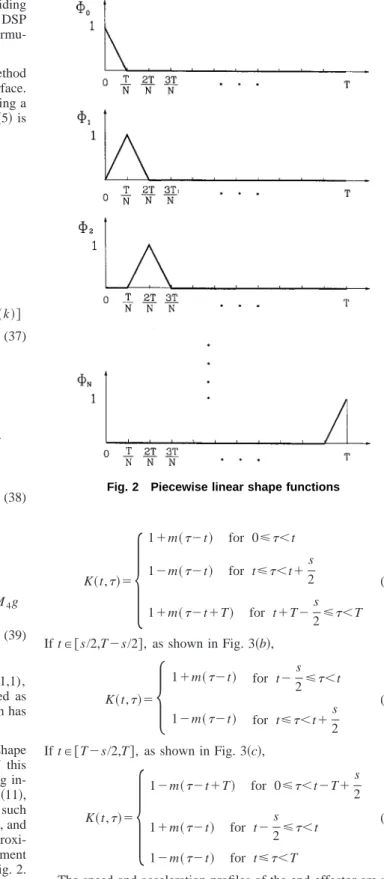
(b) The Present Method. Except for its employing shape functions to estimate influence functions, the structure of this learning control method is the same as learning control using in-tegral transforms. The learning control law consists of Eqs.共11兲, 共13兲, and 共14兲. There are some typical shape functions 关15兴 such as Fourier series shape functions, polynomial shape functions, and piecewise linear shape functions, which can be used to approxi-mate the periodic continuous function I(t,␶). This experiment employs a set of piecewise linear functions, as depicted in Fig. 2. Accordingly, in each interval of关iT/N,(i⫹1)T/N兴, only two lin-ear shape functions,⌽iand⌽i⫹1, are required; i.e., there are only

two corresponding coefficients, ciand ci⫹1, to be updated at any

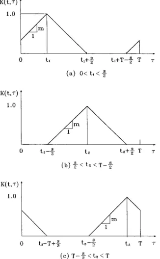
instant. For computational efficiency of a kernel function, a piece-wise linear function shown in Fig. 3 is used as a kernel function for integral transforms. The piecewise linear functions is defined as follows:

Denote the span s of this piecewise linear function as the length of a subinterval where the function value is not zero. The piece-wise linear function can be written as:

If t苸关0,s/2兴, as shown in Fig. 3共a兲,

K共t,␶兲⫽

冦

1⫹m共␶⫺t兲 for 0⭐␶⬍t 1⫺m共␶⫺t兲 for t⭐␶⬍t⫹s 2 1⫹m共␶⫺t⫹T兲 for t⫹T⫺s 2⭐␶⬍T (40) If t苸关s/2,T⫺s/2兴, as shown in Fig. 3共b兲, K共t,␶兲⫽

再

1⫹m共␶⫺t兲 for t⫺s 2⭐␶⬍t 1⫺m共␶⫺t兲 for t⭐␶⬍t⫹s 2 (41) If t苸关T⫺s/2,T兴, as shown in Fig. 3共c兲, K共t,␶兲⫽

冦

1⫺m共␶⫺t⫹T兲 for 0⭐␶⬍t⫺T⫹s 2 1⫹m共␶⫺t兲 for t⫺s 2⭐␶⬍t 1⫺m共␶⫺t兲 for t⭐␶⬍T (42)

The speed and acceleration profiles of the end-effector are pre-scribed as shown in Figs. 4共a兲 and 4共b兲, respectively. Figure 5 depicts a spatial circular trajectory to be tracked. In addition, a planar square trajectory on the X⫺Z plane, will also be carried out in experiments. Figure 6 depicts the control block diagram. To implement the present method, Eqs.共11兲, 共13兲, and 共14兲 are re-written to become the discretized form:

wˆd共k¯兲⫽ 1 2

兺

l⫽0 n⫺1 关K共k¯,l兲Iˆ共k¯,l兲⫹K共k¯,l⫹1兲Iˆ共k¯,l⫹1兲兴a⌬t (43)

Iˆ共k¯,l兲⫽

兺

i⫽0 N Cˆi共k¯,l兲⌽i共l兲 (44) Cˆi共k¯,l兲⫽Cˆ共k¯⫺1,l兲⫺KLK共k¯,l兲⌽i共l兲

兺

i⫽k⫺a⫹1 k s共i兲⌬t (45) where KL⫽diag(150,850,950), a⫽5, and integral transforms are

computed by a trapezoid method. Moreover, the sliding surface is formulated as

s共k兲⫽e共k兲⫺e共k⫺1兲

⌬t ⫹⌳e共k兲⫹⌫

兺

i⫽0

k

e共i兲⌬t (46)

where ⌳⫽diag(30,30,30), and ⌫⫽diag(30,30,30). It follows from Eq.共46兲 that the control law Eq. 共20兲 becomes, in discretized form,

u共k⫹1兲⫽⫺Q sgn关s共k兲兴⫺K关s共k兲兴⫹wˆd共k¯兲

where Q⫽diag(1,1,1), and K⫽diag(100,350,380). In this dis-crete control algorithm, k represents an index for the feedback portion of the controller, k¯ and l indexes for the repetitive learning portion, and a an integer that relates these indexes. For any given k

¯ in a period of the path, k⫽ak¯⫽al. In other words, the adapta-tion parameters cˆi are updated at a rate a times slower than the

inner feedback loop. Each increment in k represents a time step of ⌬t second, and each increment in k¯ represents a time step of a⌬t second. In both sliding mode control and the present method, the gains of the reaching law and sliding surface are the same.

Fig. 3 The piecewise linear kernel function

Fig. 4 „a…Speed profile of end-effector and„b…corresponding acceleration profile

Fig. 5 Desired spatial circular trajectory

The radius R of the desired spatial circle is denoted as 0.1 m and period T⫽10 s. The maximum speed␯maxis 0.068 m/s. The side length of the planar square is 0.1 m while the maximum speed␯maxis 0.05 m/s. A total number of 100 linear shape func-tions, i.e. N⫽100, are prescribed to approximate influence func-tions. The kernel function is a piecewise linear function of slope m⫽2; the span s of this piecewise linear function is hence 1.0 sec. 3.2 Experimental Results. To control a three-axis R-␪-Z direct-drive robot as shown in Fig. 1, which contains three servo-motors, this study employs an MX31 DSP integrated motion con-troller endowed with a TI TMS320C31 digital signal processor, as depicted in Fig. 7. Along the R axis is a direct-drive NSK Mega-thrust motor that enables the slider to undergo the force mode translational motion. For the ␪ axis, a direct-drive NSK Mega-torque motor performs the Mega-torque mode rotational motion. In ad-dition, motion along the Z axis is achieved by a 3 phase DC servo-motor operating in torque mode, where the motor rotation is altered into translation by a screw mechanism installed on the motor shaft.

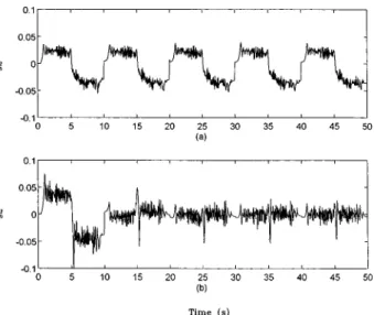
(1) Spatial Circular Trajectory Tracking. In contrast to Fig. 8共a兲, tracking errors in Fig. 8共b兲 progressively reduce to a smaller

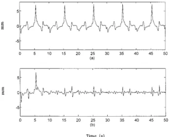
range through learning. Hence, this sliding mode based repetitive learning controller outperforms the sliding mode controller. The large tracking error generated at the beginning of the first period is arised from friction at robot joints and the prescribed acceleration command. It is difficult to quickly acquire knowledge of the fric-tion torque and the adequate motor torque corresponding to accel-eration commands at the outset of every learning period, since the learning gains can not be infinitely large during the learning pro-cess. Variation of a sliding surface is shown in Fig. 9 and confirms that the proposed control algorithm achieves its objective through learning. Using the present method, Figs. 10 and 11 depict the first time and the fifth time learning results of a spatial circular trajec-tory, respectively. There is no significant improvement after five iterations.

(2) Planar Square Trajectory Tracking. Comparing with Fig. 12共a兲 for the sliding mode control result, the tracking error shown in Fig. 12共b兲 reduces to lie between ⫾1.5 mm. Using the present method, Figs. 13 and 14, respectively, depict the first time and the fifth time learning results for the desired trajectory. The tracking accuracy is significantly improved through learning; however, the improvement after five iterations is not significant.

Fig. 7 Experimental setup

Fig. 8 Position errors inZ-axis using„a…sliding mode control and„b…the present method

Fig. 9 Sliding variables inR-axis using„a…sliding mode con-trol and„b…the present method

The overshoot error at each of four corners are mainly caused by decelerating approaching followed by accelerating departure, in addition to direction alteration of the slider.

The authors have also carried out experiments using a conven-tional controller—the PD control method. It is found that the de-parture and arrival points always do not coincide due to cumula-tive error during trajectory tracking. Moreover, concerning tracking accuracy, both PD control and the first time learning in the present method perform in a comparable manner.

4 Conclusion

This study has presented a new learning control algorithm with robust properties to improve the performance in robot tracking task. According to experimental results, the proposed control method exhibits advantages described as follows:

1 Its error convergence is faster than the sliding mode control method.

2 The time needed for the sliding surface reaching the sliding surface is shorter in each of those trajectory tracking experiments.

Fig. 10 Tracking result of the first time learning inY-Zplane

Fig. 11 Tracking result of the fifth time learning inY-Zplane

Fig. 12 Position errors inZ-axis using„a…sliding mode con-trol and„b…the present method

Fig. 13 Tracking result of the first time learning inX-Zplane

3 The accumulated errors generated at the initial time can be effectively reduced by introducing an integral term to the sliding surface.

4 The choice of shape functions depends on the trajectory to be tracked. If the polynomial order of influence functions corre-sponding to a desired trajectory is high, higher order shape func-tions, instead of current linear shape funcfunc-tions, should be adopted to improve the estimate for feedforward term.

5 Considering the coefficients adaptation law, i.e., Eq.共14兲, the proposed learning control requires fewer computer memory space since only associated coefficients for shape functions are updated at every instant.

6 The more the total number N of shape functions is used, the more accurate the feedforward term estimate can accomplish. However, for the sake of computational efficiency, N cannot be too large.

7 The proposed method using shape functions to approximate the influence function for feedforward term can be extended to higher degree-of-freedom robots in a straightforward manner, since the control algorithm for each axis undergoes its own learn-ing process uslearn-ing the same shape function set.

8 By using the modified control law Eq. 共36兲 the chattering caused by the discontinuous control law Eq.共20兲 can be improved to an acceptable extent.

9 The proposed method is robust since it can do without the dynamic model while successfully tracking the desired trajectory. References

关1兴 Arimoto, S., Kawamura, S., and Miyazaki, F., 1984, ‘‘Bettering Operation of

Robots by Learning,’’ J. Robotic Systems, 1, No. 2, pp. 123–140.

关2兴 Kwong, W. A., and Passino, K. M., 1995, ‘‘Dynamically Focused Fuzzy

Learning Control,’’ Proc. American Control Conf., pp. 3755–3759.

关3兴 Teshnehlab, M., and Watanabe, K., 1995, ‘‘Flexible Structural Learning

Con-trol of a Robotic Manipulator Using Artificial Neural Networks,’’ JSME Int. J., Series C, 38, No. 3, pp. 510–521.

关4兴 Yang, B. H., and Asada, H., 1995, ‘‘Progressive Learning for Robotic

Assem-bly: Learning Impedance with an Excitation Scheduling Method,’’ Proc. IEEE Int. Conf. on Robotics and Automation, pp. 2538–2544.

关5兴 Horowitz, R., 1993, ‘‘Learning Control of Robot Manipulators,’’ ASME J.

Dyn. Syst., Meas., Control, 115, No. 2共B兲, pp. 402–411.

关6兴 Messner, W., Horowitz, R., Kao, W. W., and Boals, M., 1991, ‘‘A New

Adap-tive Learning Rule,’’ IEEE Trans. Autom. Control., 36, No. 2, pp. 188–197.

关7兴 Guglielmo, K., and Sadegh, N., 1996, ‘‘Theory and Implementation of a

Re-petitive Robot Controller with Cartesian Trajectory Description,’’ ASME J. Dyn. Syst., Meas., Control, 118, No. 1, pp. 15–21.

关8兴 Guvenc, L., 1996, ‘‘Stability and Performance Robustness Analysis of

Repeti-tive Control Systems Using Structured Singular Values,’’ ASME J. Dyn. Syst., Meas., Control, 118, No. 3, pp. 593–597.

关9兴 Emelyanov, S. V., 1967, Variable Structure Control Systems, Nauka, Moscow 共in Russian兲.

关10兴 Slotine, J.-J. E., and Li, W., 1991, Applied Nonlinear Control, Prentice-Hall,

Englewood Cliffs, N.J.

关11兴 Gao, W., and Hung, J. C., 1993, ‘‘Variable Structure Control of Nonlinear

System: A New Approach,’’ IEEE Trans. Ind. Electron., 40, No. 1, pp. 45–56.

关12兴 Strang, G., 1980, Linear Algebra and Its Applications, 2nd ed., Academic,

Press.

关13兴 Burton, J. A., and Zinober, A. S. I., 1986, ‘‘Continous Approximation of

Variable Structure Control,’’ Int. J. Syst. Sci., 17, No. 6, pp. 876–885.

关14兴 NSK Corporation, 1989, Megatorque Motor System: User’s Manual, Tokyo,

Japan.

关15兴 Sadegh, N., Horowitz, R., and Tomizuka, M., 1990, ‘‘A Unified Approach to

Design of Adaptive and Repetitive Controllers for Robotic Manipulator,’’ ASME J. Dyn. Syst., Meas., Control, 112, No. 4, pp. 618–629.