Polynomial approximation coding for progressive image transmission

(1)

Chung-Yen Lu,1_{An-Yi Chen, and Kuei-Ann Wen} National Chiao-Tung University, Hsinchu, Taiwan, Republic of China

Received March 13, 1996

forming the coefficients. The third approach is to iteratively This paper presents a progressive image transmission scheme encode the residue or difference image, either in the spatial in which polynomial approximation coding is effectively ap- domain or in the transform domain [9–13]. At each stage, plied to encoding residual images at each stage. This polynomial _{an error or difference image is generated and then encoded} approximation coding is derived from a regressive model based _{at the next stage.}

on the relation between a set of data and their positions. Because

In this paper, a PIT system is proposed with an iterating the close relation is embedded in a certain polynomial function,

encoding technique. Residual images of variable block size the highly efficient compression can be implemented and the

are used at different stages, and they are down-sampled decimation and interpolation are also easily realized at the

to a fixed size for polynomial approximation coding (PAC). receiving side. Simulations and experimental results are

dis-The PAC is derived from a regressive model, which is a cussed in the later part of this paper. 1997 Academic Press

statistical tool for data analysis. A two-dimensional polyno-mial equation is properly suited to approximating the

rela-I. INTRODUCTION _{tion between data and their positions. Many research}

proj-ects concerned with 2D polynomial equations for 2D Progressive image transmission (PIT) has been widely _{signals have been proposed [14–18]. The PAC provides a} developed to serve many applications, such as remote im- _{simplified architecture for a PIT system with efficient} com-age data-base access, and telebrowsing and teleconferenc- _pression.

ing over relatively low bit-rate channels. Generally, trans-mission is usually divided into stages and a coarse low

II. POLYNOMIAL APPROXIMATION CODING

resolution image is transmitted as an initial approximation.

Resolution of the image is refined by sending more stages, _{Mathematically, with the techniques of polynomial} ap-and the image is transmitted progressively in order to give

proximation coding, the discrete value sets can be embed-a better embed-approximembed-ation of the originembed-al imembed-age [1–13].

ded in a continuous function f (x, y) defined on the unit Many PIT techniques have been proposed [3–13], and

square surrounding every pixel of the image. Furthermore, they can be roughly classified into three categories:

pyrami-another two-dimensional polynomial p(x, y) is employed dal, transform-based, and iterative encoding. In the

pyra-to approximate the continuous function f (x, y). That is, midal approach [3–6], the levels of the pyramid correspond

f (x, y)5 p(x, y) 1 e(x, y), where e(x, y) is the error term.

to the successive approximations of the original image.

A general type of 2D polynomial equation is p(x, y)5 The image can be progressively reconstructed by adding

_o

i

o

j bi, jxiyj, where bijare polynomial coefficients. The levels of the pyramid to the top level. In the

transform-polynomial approximation coding is based on the estima-based approach [6–9], the image first undergoes a block

tion of polynomial coefficients, followed by quantization transform and the transformed coefficients are transmitted

and variable-length coding (VLC). At the decoder, the progressively in a certain order, usually from low to high

received-bits stream is converted to a series of quantized order. In this manner, successive approximations with

pro-polynomial coefficients. These pro-polynomial coefficients are gressively higher resolution are obtained by inverse

trans-utilized to recover the original image data by the polyno-mial equation with adequate position indication (x, y). Certainly, the recovered data is an approximation result. 1

E-mail: [email protected].

317

1047-3203/97 $25.00 Copyright1997 by Academic Press All rights of reproduction in any form reserved.

(2)

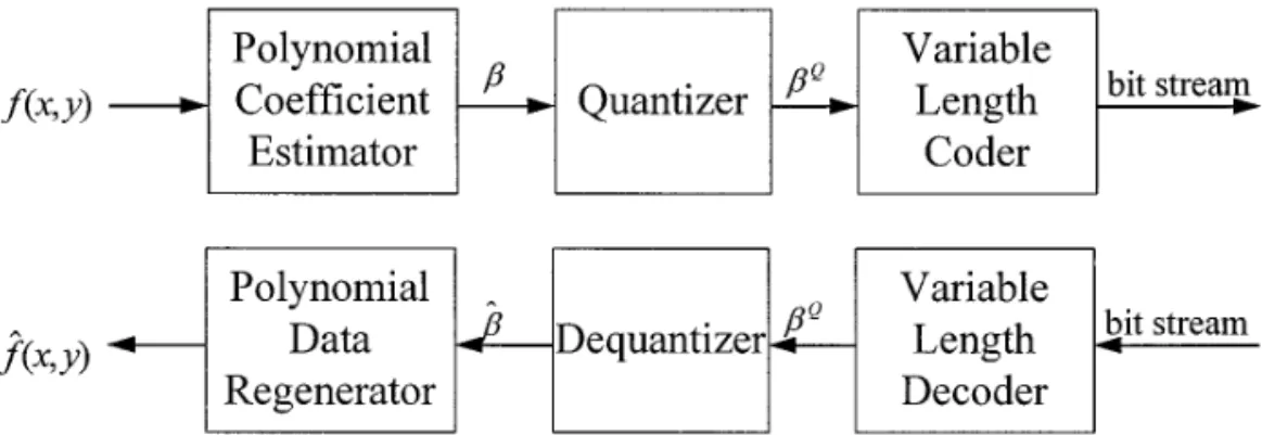
FIG. 1. The block diagram of polynomial approximation coding.

The simple block diagram that roughly describes polyno- is the constant matrix formed by position variables, mial approximation coding is illustrated in Fig. 1. The

poly-nomial-coefficient estimator (PCE) is used to estimate the bT_{5 [b}

0 b1 b2 b3] polynomial coefficient. According to the diagram, after the

stages of quantization and variable-length coding, f (x, y) _{is the coefficient matrix, and} will be transmitted in the form of encoded bit streams. At

the end of the encoder, the polynomial coefficients are _eT_{5 [e}

0 e1? ? ? en] obtained by regression techniques. The mathematical

model will be presented shortly in the later part of this _{is an error term matrix.}

section. _{After some simple numerical procedures, the}

least-Ideally speaking, the continuous function which de- _{squares estimation of the polynomial coefficient vector b}

scribes the image would be _{will be obtained with the equation}

b5 (XT_X)21_XT_F. ₍₄₎ f (x, y)5

O

y 2y

O

y 2ybm,n xm_yn_. ₍₁₎

Since the elements of X are fixed, we may replace part of Taking a 43 4 case, for example, let Eq. (4) with a generator matrix G:

G5 (XT_X)21_XT ₍₅₎

p(x, y)5

O

i

O

j

bi, jxi_yj_>b

01 b1x1 b2x1 b2y1 b3xy (2)

The computation of b will finally be expressed as and recall what was mentioned previously, that f (x, y)5

p(x, y)1 e(x, y), where e(x, y) is the error term. Now we _b_{5 GF.} ₍₆₎

define the matrix form of the polynomial approximation,

As for the decoding process, each point of the image data F5 Xb 1 e, (3) can be reconstructed according to Eq. (2). In other words, the reconstructed data matrix Fˆ of interpolation or decima-tion is directly computed by

where

Fˆ5 X

˜

b, (7)

FT_{5 [ f}

1 f2 ? ? ? fn]

where is the original data matrix with n elements,

) for X

˜

.

and x

˜

and y

˜

are the position mapping variables of extension transmission will be limited in a certain number of stages. that is, f1₅

o

m

k51fˆk1 fR, where fRis the error image in decoding for interpolation or decimation. This means, for

this m-stages system. a set of fixed polynomial coefficients, that the interpolation

Let fk_{be the input frame at the kth stage; then the input} of data is implemented by a polynomial equation with the

frame at the next stage is generated by fk11 _{5 f}k _{2 fˆ}k_. interpolation of the set of (x, y). An interpolation example

The progressively reconstructed image is expressed as of (x, y) is illustrated in Figs. 2a and 2b.

Fˆk_{5 Fˆ}k21_{1 fˆ}k_{, where Fˆ}1_{5 fˆ}1_.

Each residual frame fk_{consists of a series of}

nonover-III. PROGRESSIVE IMAGE

lapped blockshXk

l, 1# l # Nkj, where Nkis the number TRANSMISSION ALGORITHM

of blocks at frame k. The block size of each frame is varied The progressive image transmission system transmits a at different stages in order to refine the process. For the set of residual image framesh fˆk_{, k}_{. 0j. Let f}1_represent _{sake of convenience, we set Nk}

11 5 4Nk. That is, if the the original image and fˆk_{represent the transmission image} _{size of X}k_{is (2M )}_{3 (2M) at stage k, the size of X}k11_is

M3 M.

at stage k. In the ideal case, f1₅

o

k.0fk, but actually the

(4)

FIG. 4. The test image Lena of size 512_{3 512 (8 bpp) pixels.}

Step 1. Divide the frame fk _{into regular blocks, whose} The m-stage PIT algorithm is described by the

follow-ing procedures: size is N 3 N.

Step 2. Each block image is subsampled 4k21_{: 1 to the size} Step 0. Set stage variable k5 1, block size N 5 2(m11)₃

of 43 4. 2(m11)_.

TABLE 1

TABLE 2 PAC Coefficient Coding Categories

PAC Default DC Code DC Difference

Range category AC category Category Base code Length

0 00 2 0 0 21, 1 1 1 1 01 3 2 10 4 23, 22, 2, 3 2 2 27, . . . , 24, 4, . . . , 7 3 3 3 110 6 4 1110 8 215, . . . , 28, 8, . . . , 15 4 4 231, . . . , 216, 16, . . . , 31 5 5 5 11110 10 6 111110 12 263, . . . , 232, 32, . . . , 63 6 6 2127, . . . , 264, 64, . . . , 127 7 7 7 1111110 14 8 1111111 15 2255, . . . , 2127, 127, . . . , 255 8 8

(5)

0/6 11111111000 17 2/2 11110 7 0/7 11111111001 18 2/3 11111110 11 0/8 111111111000 20 2/4 11111111011 15 1/1 1101 5 2/5 111111111100 17 1/2 11100 7 2/6 111111111101 18 1/3 111110 9 2/7 111111111110 19 1/4 11111101 12 2/8 111111111111 20

Step 3. The subsampled image is encoded by PAC. Step 4. If k5 m, stop the procedure.

Step 5. Reconstruct the block image fˆk _{from PAC} de-coder.

Step 6. The residual image fk11_{is the difference between}

fk_{and fˆ}k_.

Step 7. Set k5 k 1 1, N 5 N/2, go back to Step 1. An encoder of the three-stage PIT system is illustrated in Fig. 3. Since the original image is divided into a series of nonoverlapped blocks of size 163 16 at the first stage,

m 5 3 is revealed. These blocks are downsampled to be

TABLE 4

PAC–PIT Default AC Code for Second and Third Stages

Run/ Run/

category Base code Length category Base code Length

EOB 0 1

FIG. 5. (a) Reconstructed image of size 1283 128 pixels at the

0/1 100 4 2/1 11101 6

first stage and (b) reconstructed image of size 256 3 256 at the

0/2 1100 6 2/2 1111100 9 second stage. 0/3 1101 7 2/3 111111001 12 0/4 1111010 11 2/4 11111110110 15 0/5 1111110110 15 2/5 11111110111 16 0/6 11111110000 17 2/6 11111111000 17 0/7 11111110001 18 2/7 11111111001 18

0/8 11111110010 19 2/8 11111111010 19 blocks of size 43 4 as the input of the polynomial

coeffi-1/1 101 4 3/1 111100 7 _{cients estimator; somehow the downsampling process just}

1/2 11100 7 3/2 1111101 9 _{picks up one out of every 4}_{3 4 pixels. After the}

quantiza-1/3 1111011 10 3/3 111111010 12

tion of polynomial coefficients, there are two data paths:

1/4 111111000 13 3/4 11111111011 15

one is variable length coding which is used to reduce the

1/5 1111110111 15 3/5 11111111100 16

1/6 11111110011 17 3/6 11111111101 17 bit rates; the other is inverse quantization and polynomial 1/7 11111110100 18 3/7 11111111110 18 _{data reconstruction (PDR). PDR reconstructs the block}

1/8 11111110101 19 3/8 11111111111 19

(6)

FIG. 6. (a) Reconstructed image of size 512 3 512 pixels at the first stage, (b) reconstructed image of size 512 3 512 at the second stage, and (c) reconstructed image of size 5123 512 at the third stage.

second stage, the residual image is the difference between from the previous stage is divided into nonoverlapping blocks of size 43 4 and coded by PAC.

the original image and the reconstructed image at the first stage. The residual image is divided into nonoverlapping blocks of size 8 3 8. With downsampling at the ratio of

4 : 1, PCE, quantization, and VLC are used again to encode _IV. _{EXPERIMENTAL RESULTS} the residual data. The residual image for the input at the

third stage is constructed by inverse quantization and PDR High-level language simulation using the proposed pro-gressive image transmission scheme on the test image Lena at the second stage. At the third stage, the residual image

(7)

COMPLEXITY OF PAC MSE5 1 N2

O

N21 u50

O

N21 v50 [Fˆ (u, v)2 F(u, v)]2_,

In order to design a row–column computation architec-ture, we redefine the matrix form in Eq. (3) to the form in Eq. (8):

with F and Fˆ denoting the original and reconstructed im-ages, respectively, and N the image size.

F5 XrowBXcol (8)

The PIT system transmits images in three stages. The image is first subdivided into pixel blocks of 323 32, which

are processed in left-to-right, top-to-bottom directions. As where data matrix each 323 32 block or subimage is encountered, its 1024

pixels are downsampled into a block of 43 4 pixels. Then the polynomial coefficients of this block are computed and

quantized. In particular, the nonzero AC coefficients are _F₅

3

f00 f01 f02 f03

f10 f11 f12 f13

f20 f21 f22 f23

f30 f31 f32 f33

4

, encoded using a variable-length code that defines the

coef-ficient’s value and the number of preceding zeros. The DC coefficient is differentially coded relative to the DC coefficient of the previous subimage (Table 1). Tables 2

beta matrix and 3 provide the default PAC Huffman codes at the first

stage. At the second and third stages, all the polynomial coefficients are coded by the same PAC Huffman code

B5

F

b00 b01 b10 b11

G

, listed in Table 4.

We present two sets of decoded images of different sizes. The first set of decoded images are of sizes 128 3 128,

and constant matrices 256 3 256, and 512 3 512 at three different stages. The

first two images are illustrated in Fig. 5, while the other set of decoded images are of the same size, 5123 512, as shown in Fig. 6. The bit rate and the PSNR of the coded

X5 Xrow5 Xtcol5

3

1 21.5 1 20.5 1 0.5 1 1.5

4

. images are listed in Table 5.

V. CONCLUSION

By utilizing a customized method of incorporating the

The computation of the beta matrix could be obtained polynomial regression coding for the residual images, an

with the following equation:

TABLE 5 B5 [(Xt_X)21_Xt_]F[X(Xt_X)21_]

(9) PAC–PIT and Hierarchical Mode JPEG

5 GFGt Bit-Rate vs PSNR for the Lena Image

PAC–PIT HM–JPEG [9] _where

Transmission Bit-rate PSNR Bit-rate PSNR

stage (bpp) (dB) (bpp) (dB) First stage 0.046 23.12 0.146 23.80 _G_{5 SW 5}

3

1 4 0 0 1 10

4 F

1 1 1 1 23 21 1 3

G

. (10) Second stage 0.142 26.57 0.403 28.46 Third stage 0.345 30.13 — —

(8)

18. E. Karabassis and M. E. Spetsakis, An analysis of image interpolation, Due to the scaling operation S could be merged with the

differentiation, and reduction using local polynomial fits, Graph. quantization process, only the computation of W needs to

Models Image Process. 57(3), May 1995, 183–196.

be implemented in PCE. A multiplier-free PCE architec-ture could be easily designed. Therefore, the architecarchitec-ture complexity of PAC is much less than that of the DCT-based coding algorithm.

REFERENCES

1. K. R. Sloan, Jr., and S. L. Tanimoto, Progressive refinement of Raster images, IEEE Trans. Comput. C-28 (11), Nov. 1979, 871–874. 2. P. J. Burt and E. H. Adelson, The Laplacian pyramid as a compact

image code, IEEE Trans. Comm. COM-31, Apr. 1983, 532–540. _{CHUNG-YEN LU was born in Taipei, Taiwan, R.O.C., in 1969. He} received the B.E.E., M.E.E., and Ph.D. degrees from the Department of 3. K. H. Tzou, Progressive image transmission: A review and comparison

Electronics Engineering and the Institute of Electronics Engineering at of techniques, Opt. Eng. 26, July 1987, 581–589.

National Chiao-Tung University, Taiwan, R.O.C., in 1991, 1993, and 1997, 4. L. Wang and M. Goldberg, Progressive image transmission using

respectively. Mr. Chung-Yen Lu is currently working on his post-doctoral vector quantization on images in pyramid form, IEEE Trans. Comm.

research in the area of wireless media transmission and video processing 37(12), Dec. 1989.

with the Spring Foundation of National Chiao-Tung University, Tai-5. G. Candotti and S. Carrato, Pyramidal multiresolution source coding _{wan, R.O.C.}

for progressive sequences, IEEE Trans. Consumer Electron. 40(4), Nov. 1994, 789–795.

6. K. H. Tan and M. Ghanbari, Layered image coding using the DCT pyramid, IEEE Trans. Image Process. 4(4), Apr. 1995, 512– 516.

7. K. N. Ngan, Image display techniques using the cosine transform, IEEE Trans. Acoust. Speech Signal Process. ASSP-32, Feb. 1984, 173–177.

8. E. Dubois and J. L. Moncet, Encoding and progressive transmission of still pictures in NTSC composite format using transform domain methods, IEEE Trans. Comm. COM-34, Mar. 1986, 310–319.

AN-YI CHEN was born in Tainan, Taiwan, R.O.C., in 1971. He re-9. A. Jain and S. Panchanathan, Scalable compression for image brows- _{ceived his B.E. degree from the Department of Electrical Communication} ing, IEEE Trans. Consumer Electron. 40(3), Aug. 1994, 394–404. _{Engineering at National Chiao-Tung University in 1993, and his M.S.} degree from the Department of Electrical and Computer Engineering at 10. L. Wang and M. Goldberg, Progressive image transmission by

the State University of New York at Buffalo in 1995. Presently Mr. Chen multistage transform coefficient quantization, in ‘‘IEEE International

is pursuing his Ph.D. degree at the Institute of Electronics Engineering Conference on Communications, Toronto, Ontario, June 1986,’’ pp.

at National Chiao-Tung University. His current research interests are 419–423.

image and video processing, especially compression and transmission 11. W. D. Hofmann and D. E. Troxel, Making progressive transmission

techniques. adaptive, IEEE Trans. Comm. COM-34, Aug. 1986, 806–813.

12. L. Wang and M. Goldberg, Progressive image transmission by residual error vector quantization in transform domain, in ‘‘Proc. IEEE Inter-national Phoenix Conference on Computer Communication, Scotts-dale, AZ, Feb. 1987,’’ pp. 178–182.

13. L. Wang and M. Goldberg, Lossless progressive image transmission by residual error vector quantization, IEEE Proc. 135(Pt. F5), Oct. 1988, 421–430.

14. R. M. Haralick and L. Watson, A facet model for image data, Comput. Graphics Image Process. 15, 1981, 113–129.

KUEI-ANN WEN was born in Keelung, Taiwan, Republic of China, 15. M. Eden, M. Unser, and R. Leonardi, Polynomial representation of

in 1961. She received the B.E.E., M.E.E., and Ph.D. degrees from the pictures, Signal Process. 10, 1986, 385–393.

Department of Electrical and Computer Engineering at National Cheng 16. M. Kocher and R. Leonardi, Adaptive region growing technique

Kung University, Taiwan, R.O.C., in 1983, 1985, and 1988, respectively. using polynomial functions for image approximation, Signal Process. _{She is presently a professor in the Department of Electronics Engineering,}

11, 1986, 47–60. _{National Chiao-Tung University, Hsinchu, Taiwan, R.O.C., where she}

17. M. Biggar, O. J. Morris, and A. G. Constantinides, Segmented-image has joined the Center for Telecommunications Research. Her current Coding: performance comparison with the discrete cosine transform, research interests are in the area of high-speed digital signal processing, parallel processing, and VLSI circuit design, and error correcting coding. IEEE Proc. 135(Pt. F2), Apr. 1988.